Quantum plateau of Andreev reflection induced by spin-orbit coupling

Abstract

In this work we uncover an interesting quantum plateau behavior for the Andreev reflection between a one-dimensional quantum wire and superconductor. The quantum plateau is achieved by properly tuning the interplay of the spin-orbit coupling within the quantum wire and its tunnel coupling to the superconductor. This plateau behavior is justified to be unique by excluding possible existences in the cases associated with multi-channel quantum wire, the Blonder-Tinkham-Klapwijk continuous model with a barrier, and lattice system with on-site impurity at the interface.

Andreev reflection (AR) is a remarkable and useful quantum coherent process of two particles in correlation, taking place at the normal metal/superconductor (N/S) interface And64. In this process, an incident electron in the normal metal picks up another electron below the Fermi level, forming a Cooper pair across the interface in the superconductor and leaving a hole in the normal metal dG66. Owing to its versatile applications in probing material properties, there have been intensive studies on the various AR physics and related phenomena Buz05. Very restricted examples include AR at the interface of an $s$- or a $d$-wave superconductor Dim00; Tana95 and normal systems of semiconductor DS99, ferromagnet Bee95, and spintronic material Tana06.

Of particular interest is involving spin degrees of freedom into the AR process. For instance, in the ferromagnetic/superconducting (F/S) hybrid system, an interplay of the spin degrees of freedom in the ferromagnetic material not only adds new physics to the AR process, but has created significant technique of measuring the spin polarization of magnetic materials Maz01. Another example is the N/S junction with “N” a spin-orbit coupling (SOC) system. It was found Lv12 that this hybrid system can reveal the interesting specular AR phenomena predicted in the graphene-based N/S junction where the unique band structure plays an essential role Bee06; Bee08.

In this paper we present an AR study on the hybrid system of a quantum wire with Rashba SOC interaction in contact with an $s$-wave superconductor. Instead of the popular Blonder-Tinkham-Klapwijk (BTK) continuous model (approximating the interface as a $\delta$-function potential barrier) BTK82, we perform simulation based on a lattice model. Remarkably, our simulation reveals an interesting quantum plateau behavior for this hybrid system in one-dimensional (1D) case. We justify this unique behavior by excluding its existence in the AR process associated with multi-channel quantum wire, the BTK continuous model, and 1D lattice system with on-site impurity at the interface.

Model and Methods.—

In this work we consider the hybrid system of a quantum wire with SOC interaction and in contact with a superconductor. The quantum wire is modeled as a ribbon in two dimensions, which is semi-infinite along the longitudinal $x$-direction and finite in the lateral $z$-direction. In terms of tight-binding lattice model, the wire Hamiltonian reads QF07

$$H_{\rm w} = \sum_{i}\epsilon_{i}a_{i}^{{\dagger}}a_{i}-t\sum_{i}[(a_{i}^{{\dagger}}a_{i+\delta x}+a_{i}^{{\dagger}}a_{i+\delta z})+\rm{H.c}]$$ (1)

$$+\sum_{i}[i\alpha(a_{i}^{{\dagger}}\sigma_{x}a_{i+\delta z}-a_{i}^{{\dagger}}\sigma_{z}a_{i+\delta x})+\rm{H.c}]\,.$$

Here we have abbreviated the electron operators of the $i_{\rm th}$ site with different spin orientation (in the $\sigma_{z}$ representation) in a compact form as $a_{i}^{{\dagger}}\equiv(a^{{\dagger}}_{i\uparrow},a^{{\dagger}}_{i\downarrow})$. $\alpha$ is the SOC coefficient under tight-binding lattice description, which is related to its counterpart ($\eta$) in continuous model as $\alpha=\eta/2a$ ($a$ is the lattice constant). $\epsilon_{i}$ and $t$ are the tight-binding site energy and hopping amplitude, while the nearest-neighbor hopping implies $\delta_{x}=\delta_{z}=1$.

For the superconductor we adopt a continuous Hamiltonian, in momentum $\mathbf{k}$ space which reads BTK82

$$H_{s}=\sum_{\mathbf{k},\sigma}\epsilon_{\mathbf{k}}b^{{\dagger}}_{\mathbf{k}\sigma}b_{\mathbf{k}\sigma}+\sum_{\mathbf{k}}(\Delta b^{{\dagger}}_{\mathbf{k}\uparrow}b^{{\dagger}}_{-\mathbf{k}\downarrow}+\Delta b_{-\mathbf{k}\downarrow}b_{\mathbf{k}\uparrow})\,.$$ (2)

We consider here a two-dimensional (2D) and $s$-wave superconductor. Then the order-parameter $\Delta$ (assuming real) is independent of the momentum $\mathbf{k}=(k_{x},k_{z})$. The quantum wire and the superconductor are tunnel-coupled, described as QF09

$$H^{\prime}=\sum_{i,\sigma}\left[t_{c}a^{{\dagger}}_{i\sigma}b_{\sigma}(z_{i})+{\rm H.c.}\right]\,.$$ (3)

Here, to reveal the “nearest-neighbor” coupling feature, we have converted the (superconductor) electron operator in momentum space into coordinate representation via $b_{\sigma}(z)=\sum_{k_{x},k_{z}}e^{ik_{z}z}b_{\mathbf{k}\sigma}$.

We attempt to apply the lattice Green’s function technique to compute the Andreev reflection coefficient. Since the hybrid system under study involves mixing of electron and hole, and as well their spins, it will be convenient to implement the lattice Green’s function method in a compact form of the 4-component Nambu representation QF01. In Appendix A we present the particular forms in this representation, for the quantum wire Hamiltonian and the superconductor Green’s functions (and self-energies).

Moreover, in order to implement the quantum “transport” approach based on nonequilibrium Green’s function technique for the interface Andreev reflection problem, we formally split the (semi-infinite) quantum wire into two parts: the finite part is treated as “central device”, and the remaining semi-infinite one as a “transport lead”. Then, the “central device” is subject to self-energy influences from the both (transport) leads. Based on the surface Green’s function technique, the self energy from the left lead (the SOC quantum wire) is given by Datta95

$$\Sigma_{L}^{r}(E)=H_{10}g^{r}(E)H_{01}\,.$$ (4)

Here, for simplicity, we have dropped the subscript of $H_{\rm w}$. The surface Green’s function $g^{r}(E)$ can be obtained as a self-consistent solution from the Dyson equation Datta95, $g^{r}(E)=[E-H_{00}-H_{10}g^{r}(E)H_{01}]^{-1}$. In the expressions presented here, we have labeled the first (most-left) lattice layer of the “central device” by “1”, and the most-right layer of the left lead by “0”. In general, the Hamiltonian matrix elements between them are still matrices, expanded over the lateral lattice state basis.

Analogously, applying the surface Green’s function method, in Appendix A we carry out the self energy $\Sigma^{r}_{R}$ for the effect of the right lead of superconductor. Then, the full retarded Green’s function of the central device is given by $G^{r}(E)=[E-H_{\rm w}-(\Sigma^{r}_{L}+\Sigma^{r}_{R})]^{-1}$, and the advanced one is its conjugate $G^{a}(E)=[G^{r}(E)]^{\dagger}$. Following the Keldysh nonequilibrium Green’s function technique, a lengthy algebra gives an expression for the steady-state transport current as QF09

$$I_{ss} = \frac{e}{2h}\int dE~{}\mathrm{Tr}\{[\Gamma_{L}G^{r}\Gamma_{R}G^{a}]_{ee}(f_{L}-f_{R})$$ (5)

$$~{}~{}~{}~{}~{}~{}-[\Gamma_{L}G^{r}\Gamma_{R}G^{a}]_{hh}(\bar{f}_{L}-f_{R})$$

$$~{}~{}~{}~{}~{}~{}+\Gamma_{Le}G^{r}_{eh}\Gamma_{Lh}G^{a}_{he}(f_{L}-\bar{f}_{L})$$

$$~{}~{}~{}~{}~{}~{}+\Gamma_{Lh}G^{r}_{he}\Gamma_{Le}G^{a}_{eh}(f_{L}-\bar{f}_{L})\}\,.$$

$f_{L(R)}(E)=f(E-\mu_{L(R)})$ and $\bar{f}_{L}(E)=f(E+\mu_{L})$ are, respectively, the occupied and unoccupied Fermi functions, with $\mu_{L(R)}$ the chemical potential. In the above result, “$e$” and “$h$” denote the subspace of electron and hole, which implies the spin and the lateral lattice states unresolved in explicit basis, but remaining in a $2Nc\times 2Nc$ matrix form to be traced after multiplying all the $2Nc\times 2Nc$ matrices. Finally, the rate matrix $\Gamma_{L(R)}$ in the current formula is defined from the self energy matrix via $\Gamma_{L(R)}=i[\Sigma^{r}_{L(R)}-(\Sigma^{r}_{L(R)})^{\dagger}]$, while $\Gamma_{L(R)e}$ and $\Gamma_{L(R)h}$ are their electron and hole blocks.

In Eq. (5), the first (second) term describes the electron (hole) transmission from the left to the right leads, while the third (fourth) term is for the incidence of an electron (a hole) accompanied with reflection of a hole (an electron) to the same (left) lead. Therefore, for our present interest, we extract from Eq. (5) the AR coefficient as

$$T_{A}(E)={\rm Tr}\left[\Gamma_{Le}(E)G^{r}_{eh}(E)\Gamma_{Lh}(E)G^{a}_{he}(E)\right]\,.$$ (6)

Note that this formalism has the advantage of allowing for the incident electron with arbitrary spin orientation and subject to continuous precession in the “central device”. The simulated results in this work correspond to arbitrary choice for the spin orientation of the incident electron.

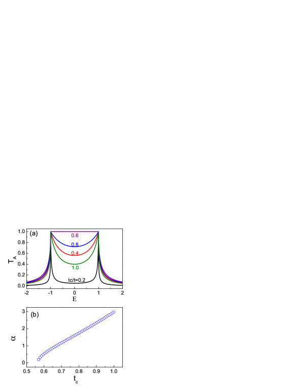
Figure 1: (color online) Quantum plateau of AR in 1D quantum wire. (a) For $\alpha=0.5t$, gradual formation of the plateau by tuning the contact coupling $t_{c}$. (b) Matching condition between the contact $t_{c}$ and the SOC $\alpha$ for the formation of the quantum plateau.

Results and Discussions.—

In our simulations, we use the tight-binding hopping energy $t$ as the units of all energies, including $E$, $t_{c}$, $\alpha$, and $\Delta$. We commonly set $\Delta=10^{-3}t$ and assume $\epsilon_{i}=\epsilon_{0}$ at the Fermi energy. In Fig. 1 we display the central result uncovered in this work for the 1D quantum wire. First, in Fig. 1(a), we visualize how a quantum plateau of the AR coefficient can appear by tuning the contact coupling $t_{c}$ to proper value, which depends on the SOC $\alpha$ as summarized in Fig. 1(b). In connection with this behavior, we mention that in the BTK paper BTK82, for an 1D wire without SOC, a similar AR plateau can appear only for vanishing $\delta$-function potential barrier, which is modeled to separate the normal and superconducting parts. In this case, the whole system is a flat 1D wire, thus the result seems not so striking, despite the right part of the wire has suffered the superconducting condensation.

In contrast, our system is inhomogeneous: the normal part is an 1D wire with SOC; and the superconducting part has no SOC. The “plateau” behavior of the AR coefficient is thus even more interesting. The proper matching condition between the SOC $\alpha$ and the contact coupling $t_{c}$ for the emergence of the quantum plateau, as displayed in Fig. 1(b), is beyond simple intuition. When satisfying this matching condition, we have checked that, by closing the superconducting gap (setting $\Delta=0$) and remaining all the other parameters unchanged, the normal transmission coefficient is unity (ideal transmission). This self consistence provides a support to the AR plateau, since the AR is anyhow a coherent tunneling process of two electrons, from the normal part into the superconductor. However, we remark that in general (the case of unmatched SOC-$\alpha$ and coupling $t_{c}$), there is no this sort of correspondence between the AR and normal transmission coefficients.

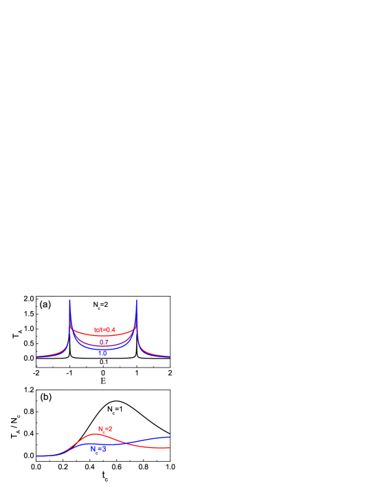
Figure 2: (color online) AR coefficient for multichannel quantum wires. (a) Results of a two-channel quantum wire where no quantum plateau is observed. (b) AR coefficient at the Fermi energy by continuously altering $t_{c}$. The results indicate no quantum plateau in the multichannel cases (e.g., $N_{c}=2$ and 3). In both (a) and (b) we set $\alpha=0.5t$.

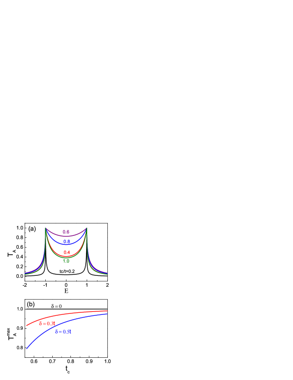
Figure 3: (color online) AR coefficient for 1D lattice wire with an impurity (with site energy $\epsilon_{\rm im}$) at the interface. (a) No quantum plateau formed for nonzero $\delta$ ($\delta=\epsilon_{\rm im}-\epsilon_{0}$). In this plot we set $\delta=0.5\,t$ and $\alpha=0.5\,t$. (b) Maximum AR coefficient ($T^{\rm max}_{A}$) at the Fermi energy by optimally matching the SOC $\alpha$ for each $t_{c}$. No quantum plateau appears for nonzero $\delta$.

The quantum plateau behavior is unique, which we found exists only for 1D SOC quantum wire. We justify this by simulating multichannel quantum wires, with results as shown in Fig. 2. In Fig. 2(a) and (b), for a given SOC $\alpha$, by altering the contact coupling $t_{c}$, the quantum plateau can no longer be tuned out now. As a complementary plot, we show in Fig. 2(c) the AR coefficient at the Fermi energy ($E=0$). For comparative purpose, we rescale the AR coefficient as $T_{A}/N_{c}$, since for the multichannel quantum wire the AR coefficient (the sum of multiple scattering channels) can exceed unity. Clearly, we see that, only in the 1D case ($N_{c}=1$), can a proper tuning of the contact coupling ($t_{c}$) and the SOC $\alpha$ result in the quantum plateau behavior. In contrast, for multichannel wires (e.g., $N_{c}=2$ and 3), the quantum plateau cannot be tuned out, as demonstrated in Fig. 2(c) by noting that at the edge ($E=\pm\Delta$), the AR coefficient is “$N_{c}$” (the lateral channel numbers).

We further justify the quantum plateau behavior by considering the BTK 1D continuous model BTK82. The BTK model assumes a normal quantum wire connecting with a superconductor through a $\delta$-potential barrier (with height $V_{0}$). In our case, we further consider the quantum wire with the Rashba SOC interaction (with strength $\eta$). In Appendix B, we present a detailed solution for this system and obtain the AR coefficient as

$$T_{A}=\frac{(1+x^{2})(4Z_{2}^{2}+1)}{(4Z_{2}^{2}+1)+x^{2}(2Z_{1}^{2}+2Z_{2}^{2}+1)^{2}}\,,$$ (7)

where $Z_{1}=\frac{mV_{0}}{\hbar^{2}k_{F}}$ and $Z_{2}=\frac{m\eta}{2\hbar^{2}k_{F}}$, with $m$ the electron mass and $\hbar k_{F}$ the Fermi momentum. Also, for $E\leq\Delta$, we have introduced the dimensionless parameter $x=(\Delta^{2}-E^{2})^{\frac{1}{2}}/E$. From Eq. (7), one can check that $T_{A}=1$ only at $E=\Delta$, and $T_{A}(E)<1$ for other $E$. So we conclude that the quantum plateau behavior does not appear in the BTK model for nonzero height of barrier.

To understand the above result, which seems in contrast with the result observed earlier in Fig. 1, let us return to the 1D lattice model. The $\delta$-potential barrier, in certain sense, is analogous to an “impurity” at the end of the 1D lattice chain, through which the quantum wire is coupled to the superconductor. Based on this sort of “impurity” model, we perform further simulations and present the results in Fig. 3. In Fig. 3 (a) we show that, for a given SOC $\alpha$ and altering the contact coupling ($t_{c}$), one can no longer tune out the quantum plateau for the AR coefficient. Indeed, this differs from what we observed in Fig. 1, but is in consistence with the BTK model discussed above. In Fig. 3 (b) we present a more complete plot for the absence of the quantum plateau. For several impurity site-energies ($\epsilon_{\rm im}$), we display how the quantum plateau behavior disappears. In this plot, we employ the maximum value ($T^{\rm max}_{A}$) of the AR coefficient at the Fermi energy, by optimally tuning the SOC $\alpha$ for each $t_{c}$, to illustrate the behavior.

Concluding Remarks.—

We thus arrive at a conclusion that the quantum plateau of AR can be formed for a homogeneous 1D wire in contact with a superconductor, as a result of participation of the SOC interaction in the quantum wire. For this behavior, the SOC effect is essential and not obvious. First, the incident electron can be initially in arbitrary spin orientation and experiences continuous spin precession during its propagation. Second, at the interface, two electrons with opposite spins coherently enter the superconductor and form a Cooper pair. But the superconductor is of invariance under spin rotations, having no unique preferring direction for spin. This likely leads to an intuition: the AR should not be affected by the SOC interaction in the quantum wire. However, our result reveals that the SOC-induced spin precession, spatially away from the interface, does affect the two-electron tunneling into the superconductor and even a quantum plateau can be induced. The AR plateau also implies a SOC-induced “transparency” for the interface, which does not cause normal reflections.

To summarize, in this work we predict a quantum plateau behavior for the Andreev reflection in 1D quantum wire system, associated with spin-orbit coupling. It would be of interest to verify this behavior by experiment in possible engineered 1D systems.

Appendix A Particulars in Nambu Representation

The hybrid system under present study involves mixing of electron and hole, together with their spins. Let us introduce a generalized Nambu representation QF01, $\psi_{i}=(a_{i\uparrow},a_{i\downarrow},a^{\dagger}_{i\downarrow},a^{\dagger}_{i\uparrow})^{T}$, for the electron operators of the $i_{\rm th}$ layer lattice sites along the lateral ($z$) direction. The quantum wire Hamiltonian can be reexpressed in a compact form as

$$H_{\rm nw}=\frac{1}{2}\sum_{i}\left[\psi^{\dagger}_{i}H_{i,i}\psi_{i}+\left(\psi^{\dagger}_{i}H_{i,i+1}\psi_{i+1}+{\rm H.c.}\right)\right]\,.$$ (8)

First, the Hamiltonian matrix $H_{i,i+1}$ reads

$$H_{i,i+1}=\begin{bmatrix}-\widetilde{t}_{+}&0&0&0\\ 0&-\widetilde{t}_{-}&0&0\\ 0&0&\widetilde{t}_{+}&0\\ 0&0&0&\widetilde{t}_{-}\end{bmatrix}\bigotimes I_{Nc\times Nc}\,,$$ (9)

where $\widetilde{t}_{\pm}=t\pm i\alpha$. The second Hamiltonian matrix, $H_{i,i}$, has three parts: $H_{i,i}=H_{0}+H_{1}+H_{2}$. Each is given by, respectively,

$$H_{0}=\begin{bmatrix}\epsilon_{i}&0&0&0\\ 0&\epsilon_{i}&0&0\\ 0&0&-\epsilon_{i}&0\\ 0&0&0&-\epsilon_{i}\end{bmatrix}\bigotimes I_{Nc\times Nc}$$ (10)

$$H_{1}=\begin{bmatrix}-t&0&0&0\\ 0&-t&0&0\\ 0&0&t&0\\ 0&0&0&t\end{bmatrix}\bigotimes\begin{bmatrix}0&1&\\ 1&0&\ddots&\text{{\huge{0}}}\\ &\ddots&\ddots&\ddots&\\ &&\ddots&0&1\\ &\text{{\huge{0}}}&&1&0\end{bmatrix}_{Nc\times Nc}$$ (11)

$$H_{2}=\begin{bmatrix}0&\alpha&0&0\\ \alpha&0&0&0\\ 0&0&0&\alpha\\ 0&0&\alpha&0\end{bmatrix}\bigotimes\begin{bmatrix}0&i&\\ -i&0&\ddots&\text{{\huge{0}}}\\ &\ddots&\ddots&\ddots&\\ &&\ddots&0&i\\ &\text{{\huge{0}}}&&-i&0\end{bmatrix}_{Nc\times Nc}$$ (12)

Similarly, for the superconductor (Hamiltonian and Green’s functions), we introduce the 4-component Nambu representation $\psi^{{\dagger}}_{s}=(b^{\dagger}_{\uparrow},b^{\dagger}_{\downarrow},b_{\downarrow},b_{\uparrow})$. Originally, the electron operators in the superconductor Hamiltonian, Eq. (2), are defined in momentum space. For the purpose of applying the surface Green’s function technique, we introduce the “surface” electron operator via $b_{\sigma}(z)=\sum_{k_{x},k_{z}}e^{ik_{z}z}b_{\mathbf{k}\sigma}$. In this representation, the (retarded) surface Green’s function of the superconductor reads QF01

Applyingtheequation-of-motionmethod,infrequencydomainoneobt