Accurate Local Estimation of Geo-Coordinates for Social Media Posts

Abstract

Associating geo-coordinates with the content of social media posts can enhance many existing applications and services and enable a host of new ones. Unfortunately, a majority of social media posts are not tagged with geo-coordinates. Even when location data is available, it may be inaccurate, very broad or sometimes fictitious. Contemporary location estimation approaches based on analyzing the content of these posts can identify only broad areas such as a city, which limits their usefulness. To address these shortcomings, this paper proposes a methodology to narrowly estimate the geo-coordinates of social media posts with high accuracy. The methodology relies solely on the content of these posts and prior knowledge of the wide geographical region from where the posts originate. An ensemble of language models, which are smoothed over non-overlapping sub-regions of a wider region, lie at the heart of the methodology. Experimental evaluation using a corpus of over half a million tweets from New York City shows that the approach, on an average, estimates locations of tweets to within just $2.15$km of their actual positions.

1 Introduction

The information shared by users over Online Social Networks (OSNs) such as Facebook and Twitter offer unique insights into their thoughts, emotions, and opinions. The richness of these posts has motivated numerous organizations to harvest the content embedded within them in support of value-added services. Associating geographic locations with the information extracted from these posts can offer both theoretical and practical benefits. Theoretically, this association can facilitate sociological studies to examine how online behaviors, relationships, and interactions are influenced by their offline socio-spatial counterparts [17]. Practically, the linking of location to content can enhance existing services such as location-based advertising [12] and disaster response [20] and conceive novel ones.

Social media posts may be tagged with location information in two ways. First, users may choose to automatically tag their posts shared via GPS-enabled mobile devices. Second, many OSNs allow users to include their current location [16] through fields such as “location” or “from” in their social media profiles. If users diligently and authentically use one of these two methods, then accurate location information can be extracted easily. However, currently, a vast majority of users do not enable tagging of their mobile posts [4] and choose not to include their locations in their profiles, perhaps for privacy reasons. Some users who do populate this field may specify it broadly in terms of a state or a country, while some may intentionally provide inaccurate or fictitious positions [9]. Thus, in practice, only a small percentage of social media posts are accompanied by rich and accurate location data. To alleviate this shortcoming, contemporary approaches that need the location of posts estimate it by analyzing their content. These approaches, however, estimate broad regions of the order of a city, or location “types” such as restaurants, offices, homes, or stores [6, 13]. Finally, a few efforts that try to estimate the actual positions or geo-coordinates of social media posts are accurate within a radius of 80-100 km [4, 14, 5], essentially identifying only broad regions.

Once the broad region from where a social media post has originated is identified either through tagging, by finding keywords corresponding to famous landmarks and interesting events, or by using an aforementioned contemporary approach, pinning it down narrowly to within a small radius around its actual geo-coordinates may add significant value. For example, such local geo-tagging can shed light on how people within a neighborhood think similarly as they are exposed to common events, and participate in richer and meaningful offline friendships [15]. Identifying localities can also provide more accurate information on an event or a disaster which can be highly beneficial to first responders [20]. Law enforcement can also use such fine geo-tagging to approximate the location of a suspect, who is known to be present in a town or a city. Finally, it may be feasible to identify the geo-coordinates of a post with high accuracy once its broad region is known because this prior knowledge limits the range of possible positions.

In this paper, we present a methodology to accurately estimate the geo-coordinates of a social media post based on its content, once the broad region from where it originates is known. The methodology consists of partitioning the broad region into a grid of non-overlapping sub-regions, building probabilistic language models over each sub-region, and then applying geo-smoothing to improve the accuracy of the location estimates. We train and evaluate the language models over a corpus of tweets collected across downtown and midtown Manhattan, and find that the approach, on an average, pinpoints the positions of tweets to within $2.15$km, or just 4% of the size of the total region from which they are known to originate.

This paper is organized as follows. Section 2 describes our estimation methodology. Section 3 presents experimental evaluation. Related work is compared in Section 4. Conclusions and future work are offered in Section 5.

2 Estimation Methodology

In this section, we describe the two steps in the methodology to estimate geo-coordinates.

2.1 Building Language Models

The topics, thoughts, words, and expressions embedded within social media posts are influenced by the inherent properties and circumstances of the locality from where users share these posts. For example, people may share their opinions of a restaurant while seated there. They may also share about an accident or a noteworthy public event as it occurs. The culture and social norms of a local area may also modulate these posts. As an example, posts from Little Italy in New York City may be pre-dominantly influenced by Italian norms and culture, while those from Times Square may instead overwhelmingly share the excitement of visiting the city. Thus, both the language and the content of social media posts shared from different, smaller sub-regions within a broad region will be varied.

To expose these local variations, we partition a broad region of interest $\mathcal{L}$ into a collection of equally sized, non-overlapping sub-regions $\ell_{i}$, which are defined by a $g\times g$ grid. We then build an ensemble of models; one per sub-region to represent the language of its posts. This ensemble is inspired by recent approaches including our own [7, 8], that have demonstrated its promise in capturing the linguistic variations in the content of social media posts. A language model defines a probability distribution over $n$-grams, where an $n$-gram is an ordered sequence of $n$ words $(w_{1},....,w_{n})$. The maximum likelihood estimate of an $n$-gram, computed over a corpus of posts within $\ell_{i}\in\mathcal{L}$, is given by [1]:

$$P_{\ell_{i}}(w_{1},...,w_{n})=\frac{c_{\ell_{i}}(w_{1},...w_{n})}{c_{\ell_{i}}(w_{1},...,w_{n-1})}$$

where $c(.)$ is the number of times the sequence appears in the posts. The probability that a sub-region generates a phrase $T=(w_{1},...,w_{k})$ is computed as the product of the probabilities of the $n$-grams that comprise $T$:

$$P(T|\ell_{i})=\prod_{j=1}^{k-n+1}P_{\ell}(w_{j},w_{j+1},...,w_{j+n-1})$$

Contextual information increases with $n$ because longer sequences of words can be considered. However, because social media posts are short, specific long word sequences appear with low frequency, and hence, prevalent approaches use only unigrams to model these posts. Although unigrams or $1$-grams model the distinct vocabulary, independent of the order of words [2], they lack the ability to capture context within a language. For example, a unigram model trained over “going to work” can represent how one discusses the concept of “work”, and the action of “going”, but cannot associate the concept with the action. Language models trained over bigrams “going to” and “to work”, however, can capture additional context of going somewhere, and applying an action or a verb to the concept of “work”. We limit to bigrams although higher order models can capture even more details, because estimating higher order models may be inaccurate using a corpus of social media posts that are typically short but refer to a broad variety of topics.

To improve the accuracy of the language models, we interpolate the probability of a bigram with the probability of the unigram that completes it. This interpolation compensates for the low count of a bigram by incorporating the expected higher count of the unigram that completes it. For example, if the unigram “driving” is used frequently in a training corpus, we should expect that bigrams completed by this word (e.g. “love driving”) are more likely to be seen even if the bigram does not appear often. Thus, for a sub-region $\ell_{i}$, the probability of observing the bigram $(w_{j-1},w_{j})$ is given as:

$$P_{\ell_{i}}(w_{j-1},w_{j})=\lambda_{1}\frac{c(w_{j-1},w_{j})}{c(w_{j-1})}+\lambda_{2}\frac{c(w_{j})}{|W(\ell_{i})|}$$

where $\lambda_{1}+\lambda_{2}=1$, $|W(\ell_{i})|$ is the number of distinct words in all posts in $\ell_{i}$ and $c(w_{j})/|W(\ell_{i})|$ is the estimate of the unigram that completes the bigram [1].

We further compensate the language model to account for future unseen bigrams by diverting some of the probability of the training bigrams to those that are as yet unobserved. We use the Modified Kneser-Ney (MKN) algorithm [11] for this compensation because it offers the best performance for interpolated language models [3]. The MKN algorithm subtracts a constant $\hat{d}$ from the observed frequency of every known bigram. It then estimates the likelihood that an unknown bigram $(w_{j-1},w_{j})$ will appear with a modified estimate of the unigram $w_{j}$, where only the number of distinct bigrams that $w_{j}$ completes is considered:

$$P_{c}(w_{j})=\frac{|\{w:c(w,w_{j})>0\}|}{\sum_{v}|\{w:c(w,v)>0\}|}$$

$P_{c}(w_{j})$ is then weighted by the probability mass $\lambda(w_{j-1})$ that is taken by subtracting $\hat{d}$ from the counts of known bigrams:

$$\lambda(w_{j-1})=\frac{\hat{d}|\{w:c(w_{j-1},w)>0\}|}{c(w_{j-1})}$$

Thus, under the MKN algorithm the probability of observing a bigram becomes:

$$P_{\ell_{i}}(w_{j-1},w_{j})=\frac{\max(c(w_{j-1},w_{j})-\hat{d},0)}{c(w_{j-1})}+\lambda(w_{j-1})P_{c}(w_{j})$$

If $(w_{j-1},w_{j})$ is unknown, the probability is just given by $\lambda(w_{j-1})P_{c}(w_{j})$, and if it is known, the probability is given as a linear interpolation of the modified bigram and unigram estimates. Note that the modified unigram estimate $P_{c}(w_{j})$ is superior to $c(w_{j})/|W(\ell)|$ because under $P_{c}(w_{j})$, words that appear frequently but within few distinct contexts will not strongly influence the probability of the bigram. We estimate $\hat{d}$ such that the log-likelihood that the model generates a given bigram is maximized:

$$\hat{d}=\arg\max_{d}\sum_{v}c(v,w_{j})\log P_{\ell}(v,w_{j})$$

This has a closed form approximation depending on whether $c(w_{i-1},w_{i})$ is equal to $1$, $2$, or $\geq 3$ [19]. Using these approximations, we set $\hat{d}$ equal to $d_{1},d_{2}$, or $d_{3}$ respectively: $d_{1}=1-(2n_{2}/(n_{1}+2n_{2}))$, $d_{2}=2-(3n_{3}n_{1}/(n_{2}(n_{1}+2n_{2})))$, and $d_{3}=3-(4n_{4}n_{1}/(n_{3}(n_{1}+2n_{2})))$ where $n_{i}$ is the number of bigrams that appear with frequency $i$. Subsequently, we define the probability that a social media post $T$ is generated from a sub-region $\ell_{i}$ $P(T|\ell_{i})$ as:

$$P(T|\ell_{i})=\prod_{j=2}^{k}P_{\ell_{i}}(w_{j-1},w_{j})$$

2.2 Estimating Geo-Coordinates

After training the language models over tweets from each sub-region, the ensemble is queried to compute the probability that a social media post $T$ is generated from a sub-region $\ell_{i}$ using Bayes rule:

$$P(\ell_{i}|T)=\frac{P(T|\ell_{i})P(\ell_{i})}{\sum_{j}P(T|\ell_{j})P(\ell_{j})}$$

$P(\ell_{i})$ is the prior probability that a social media post is from sub-region $\ell_{i}$ and is given by $N(\ell_{i})/N(\mathcal{L})$. $N(\ell_{i})$ is the number of posts in $\ell_{i}$ and $N(\mathcal{L})$ is the total number of posts in the entire city $\mathcal{L}$. The geo-coordinates of a post $T$ may be estimated as the center of the sub-region whose posterior probability $P(\ell_{i}|T)$ is the highest, that is, we may choose the center of $\ell^{*}$ where $\ell^{*}=\arg\max_{i}P(\ell_{i}|T)$.

Previous works suggest that the proximity to an object increases the propensity of the users to post about it [6, 18]. In other words, it is feasible that the language of a sub-region may be influenced by the landmarks and events within its neighboring sub-regions. Thus, although we can naively use the highest $P(\ell_{i}|T)$ to estimate the geo-coordinates of a post, we introduce a geo-smoothing function $\Theta^{\circ}(\ell_{i}|T)$, which combines the posterior probabilities of the neighboring sub-regions to capture their influence on the language in $\ell_{i}$. Based on this geo-smoothing function, we select $\ell^{*}$ as $\ell^{*}=\arg\max_{i}\Theta^{\circ}(\ell_{i}|T)$. Popular functional forms for $\Theta^{\circ}$ include a decay component that reduces the contribution of neighbors as they get increasingly away from $\ell_{i}$ [13]. Such geo-smoothing performs best when the decay component takes a polynomial form [6, 18]. Thus, in this preliminary study, we consider the simplest polynomial shown to be effective in geo-locating documents [18]. Letting $\Omega_{k}(\ell_{i})$ be the set of neighbors of $\ell_{i}$ whose distance is $k$ cells away, and $P_{\ell_{i}}(T)=P(\ell_{i}|T)$, our geo-smoothing function is defined as:

$$\begin{split}&\Theta^{\circ}(P_{\ell_{i}}(T);\alpha,d)=(1-\alpha)P_{\ell_{i}}(T)\\ &\quad\quad{}+\alpha\sum_{k=1}^{d}\sum_{\omega\in\Omega_{k}(\ell_{i})}\frac{P_{\omega}(T)}{(2k+1)^{2}-1}\end{split}$$

where $\alpha\in[0,1]$ is the smoothing weight and $d$ is smoothing diameter, that is, the largest distance from which a neighbor can be located.

It is important to note that the accuracy of the estimated geo-coordinates is limited to the resolution of the $g\times g$ grid chosen to divide the region into sub-regions. Increasing $g$ will decrease the size of the sub-regions and allow for more accurate estimation, however, the number of posts available within each sub-region may be insufficient to train the models. On the other hand, decreasing $g$ increases the size of individual sub-regions so that they contain more posts, but limits the estimation accuracy. Similarly, increasing $\alpha$ and $d$ respectively increase the importance and number of the neighboring sub-regions. If $\alpha$ and $d$ are very high, neighboring sub-regions may dwarf the candidate sub-region. However, if they are too low, they may not adequately capture users’ reactions on the local events and objects. We empirically choose the values of the three hyperparameters $g$, $\alpha$ and $d$ to balance these competing concerns.

3 Experimental Evaluation

In this section, we describe the data, its pre-processing, hyperparameter fits, and evaluation results.

3.1 Data Pre-Processing

We collected over half-million geo-tagged tweets using Twitter’s Streaming API  across New York City over a three-month period (January 29th - April 7th, 2013). The tweets were collected across a $51.44$km² region that includes downtown and midtown Manhattan because it includes popular residential and commercial districts as well as tourist destinations. We expect that because of this diversity tweets from this region will capture varied thoughts representing the perspectives of long-term city residents, commuters, and visitors.

For every tweet, we eliminated all non-English words and characters. We also eliminated hashtags because although they may indicate topic and content, they may also include shorthand or concatenated words (i.e. “#WestEnd”) that the language models cannot decipher. We further pre-processed the tweets by converting all words to lowercase and by stripping punctuation, username replies, and links to Web pages. We also produced a stopword list of the $200$ most frequently used words such as “at”, “the”, and “or”, which lack contextual information, and hence, introduce noise into the estimation of bigrams. We choose a limited stopword list that is approximately equal to $1\%$ of the number of distinct words across the data collection region. We also include a “catch all” unigram “$<$misc$>$” to aggregate the probability of words that occur only once. This term thus accounts for the many miscellaneous, shorthand, mis-spelled, and other user-specific notations that are uniquely common to Twitter. Of the 574,948 tweets, we reserved 408,095 ($70\%$) for training the language models, 83,990 ($15\%$) for evaluation, and another 82,863 ($15\%$) as hold-out data for fitting the hyperparameters.

3.2 Hyperparameter Fits

We find values for the three hyperparameters, namely, the grid size $g$, smoothing weight $\alpha$, and smoothing diameter $d$ such that the average estimation error of $\Theta^{\circ}$ across the set of hold-out tweets is minimized. We define the average estimation error as the geo-distance (in km) between the actual GPS coordinates of a tweet to the center of the sub-region that the model estimates it is from. The parameters were fit via a standard grid search where $\alpha$ and $d$ were varied within their range of possible values, namely, $\alpha\in\{0.1,0.2,...,1.0\}$ and $d\in\{1,...,g\}$. We chose to vary $g\in\{5,6,...,15\}$ because the estimation error increased when $g$ was outside this range regardless of $\alpha$ and $d$.

As we simultaneously varied $\alpha$, $d$, and $g$ in these ranges, we found that irrespective of $g$ and $d$, $\alpha=0.9$ consistently minimized the estimation error. In other words, only $10\%$ of the posterior probability that a tweet $T$ originated from a sub-region $\ell_{i}$ can be attributed to its own language model $P_{\ell_{i}}(T)$, while the rest is contributed by the language models of the neighboring sub-regions. Furthermore, for every value of $g$, estimation error over the hold-out set is minimized at $d=g$. We thus set the grid size parameter $g$ equal to $d$ and $\alpha=0.9$. Figure 1 shows the mean error for different values of $g$. We achieve the best performance across the hold-out data when we set $g=8$, where the city is partitioned into 64 sub-regions each with an area $0.803$km². With $g$ set to $8$ and $\alpha=0.9$, we then estimate the the parameters of the interpolated bigram language models using the method described in Section 2.

Figure 1: Mean Hold-out Errors – $\alpha=0.9$, $d=g$

3.3 Evaluation Results

We experimentally explore the influence of $d$ on the overall estimation error over the test set comprising 82,863 tweets. Table 1 shows that the average estimation error decreases as $d$ rises. Thus, even a simple polynomial function can appropriately decay probabilities from sub-regions as they get farther away from $\ell_{i}$ and significantly enhance estimation accuracy. We note that the mean error does not change for $d\geq 5$ because as the diameter of geo-smoothing increases to include sub-regions $d=g/2$ cells away, central sub-regions in the city begin to consider almost every other sub-region in its set of neighbors. Further increases in $d$ thus do not change $P_{\ell_{i}}(T)$ for a growing number of sub-regions, causing the mean estimation error to converge.

Diameter	$1$	$2$	$3$	$4$	$5+$
Mean Error	$3.38$	$2.39$	$2.18$	$2.16$	$2.15$

Table 1: Mean Estimation Error (km)

We evaluate the distribution of error estimates as a function of $d$ in in Figure 2. At $d=1$, where only directly adjacent neighbors are considered, the estimation errors are bi-modal with small peaks at approximately $0.7$km and $3.8$km. The error distribution has a very wide variance; except for a decrease between $1$ and $3$km, the error terms are generally distributed uniformly in the range $0$ and $6$km. The bi-modal behavior disappears for $d=2$ and most of the mass accumulates at errors less than than $2$km. For $d=3$, the peak sharpens even further at approximately $1.75$km, which is less than the mean estimation error of $2.18$km. The densities for $d\geq 3$ are nearly identical because the estimates change only for a very small number of tweets as $d$ increases from $1$ to $3$.

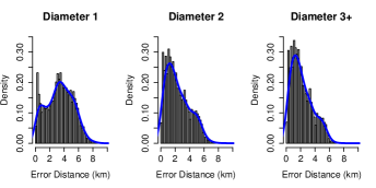
Figure 2: Error Densities vs. $d$

Finally, we evaluate how frequently our model is accurate to within a given distance in Figure 3, where we plot the CDF of estimation errors for $d=1,2,$ and $\geq 3$ on semi-log scale. The shape of the distribution function becomes linear for $d>2$, which suggests that the density function takes an exponential form as the smoothing diameter increases. We also find that the estimation accuracy increases only marginally beyond $d\geq 2$, suggesting that smoothing over neighbors more than $2$ sub-regions away offers diminishing returns. Furthermore, the semi-log plots confirm monotonic behavior. In other words, there is no special case or specific instance for which a smaller value of $d$ outperforms a larger value $d$. The overall accuracy of our approach is promising; at $d=3$ the model can estimate the geo-coordinates of a tweet to within $4$km with probability $80\%$, to within $2$km at over $50\%$, and to within $1$km at $20\%$.

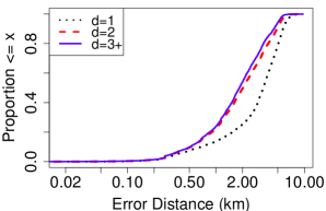
Figure 3: Error Distributions

4 Related Research

In this section, we review contemporary techniques according to whether they estimate the locations or geo-coordinates of social medial posts.

Broadly, the techniques that identify user locations either zero in on the “home” locations of users or location “types” from where users check-in and update. These methods rely on spatial word usage and language models [6], posting behaviors and external data on locations [14], and inferences based on unified discriminative models [13]. Estimation of specific geo-coordinates also use varied techniques including language models [18, 4], spatial word distributions [4], sequences of check-ins from social network friends [16], integrating mobile phone data [5], and mapping latent topics from across regions [10].

Despite the integration of data from separate sources, and the aid of sophisticated probabilistic models, both types of approaches can identify only broad areas. By contrast, the methodology proposed in this paper can narrowly estimate geo-coordinates while relying solely on the content of the posts and on prior knowledge about the wide area from where they originated.

5 Conclusions & Future Work

In this paper, we presented a methodology to narrowly estimate the geo-coordinates of a social media post, given the knowledge of the much broader region from where they originate. An experimental evaluation using tweets collected from New York City shows that on an average the methodology can estimate geo-coordinates of social media posts to within $2.15$km, or just 4% of the size of the broader region. Future work will examine the accuracy of the approach over regions with distinct geographic features, sizes, and population distributions. We also propose to investigate the accuracy of alternative geo-smoothing methods.

References

- [1] L. R. Bahl, F. Jelinek, and R. L. Mercer. A maximum likelihood approach to continuous speech recognition. IEEE Transactions on Pattern Analysis and Machine Intelligence, (2):179–190, 1983.
- [2] S. Chandra, L. Khan, and F. Muhaya. Estimating twitter user location using social interactions–a content based approach. In Intl. Conf. on Social Computing, pages 838–843. IEEE, 2011.
- [3] S. Chen and J. Goodman. An empirical study of smoothing techniques for language modeling. In Proc. of Association for Computational Linguistics Annual Meeting, pages 310–318. Association for Computational Linguistics, 1996.
- [4] Z. Cheng, J. Caverlee, and K. Lee. You are where you tweet: a content-based approach to geo-locating twitter users. In Proc. of Intl. Conference on Information and knowledge management, pages 759–768. ACM, 2010.
- [5] E. Cho, S. A. Myers, and J. Leskovec. Friendship and mobility: user movement in location-based social networks. In Proc. of Intl. conference on Knowledge discovery and data mining, pages 1082–1090. ACM, 2011.
- [6] N. Dalvi, R. Kumar, and B. Pang. Object matching in tweets with spatial models. In Proc. of Intl. Conference on Web search and data mining, pages 43–52. ACM, 2012.
- [7] D. Doran, S. Gokhale, and A. Dagnino. Human Sensing for Smart Cities. In Proc. of Intl. Conf. on Advances in Social Network Analysis and Mining, pages 1323–1330, 2013.
- [8] D. Doran, S. Gokhale, and A. Dagnino. Understanding Common Perceptions from Online Social Media. In Proc. of Intl. Conference on Software Engineering and Knowledge Engineering, pages 107–112, 2013.
- [9] B. Hecht, L. Hong, B. Suh, and H. E. Chi. Tweets from justin bieber’s heart: the dynamics of the location field in user profiles. In Proc. of Intl. Conference on Human Factors in Computing Systems, pages 237–246. ACM, 2011.
- [10] L. Hong, A. Ahmed, S. Gurumurthy, A. J. Smola, and K. Tsioutsiouliklis. Discovering Geographical Topics in the Twitter Stream. In Proc. of Intl. Conf. on World Wide Web, pages 769–778, 2012.
- [11] R. Kneser and H. Ney. Improved backing-off for m-gram language modeling. In Intl. Conference on Acoustics, Speech, and Signal Processing, volume 1, pages 181–184. IEEE, 1995.
- [12] B. Kolmel and S. Alexakis. Location based advertising. In Intl. Conference on Mobile Business, 2002.
- [13] R. Li, S. Wang, H. Deng, R. Wang, and K. C.-C. Chang. Towards social user profiling: unified and discriminative influence model for inferring home locations. In Proc. of Intl. Conference on Knowledge discovery and data mining, pages 1023–1031. ACM, 2012.
- [14] J. Mahmud, J. Nichols, and C. Drews. Where is this tweet from? inferring home locations of twitter users. In Proc. of Intl. Conference on Weblogs and Social Media, volume 12, pages 511–514, 2012.
- [15] D. Mok, B. Wellman, and J. Carrasco. Does distance matter in the age of the internet? Urban Studies, 47(13):2747–2783, 2010.
- [16] A. Sadilek, H. Kautz, and J. Bigham. Finding Your Friends and Following Them to Where You Are. In Proc. of Intl. Coference on Web Search and Data Mining, pages 723–732, 2012.
- [17] S. Scellato, A. Noulas, R. Lambiotte, and C. Mascolo. Socio-spatial properties of online location-based social networks. In Proc. of Intl. Conference on Weblogs and Social Media, volume 11, pages 329–336, 2011.
- [18] P. Serdyukov, V. Murdock, and R. Van Zwol. Placing flickr photos on a map. In Proc. of Intl. Conf. on Research and Development in Information Retrieval, pages 484–491, 2009.
- [19] M. Sundermeyer, R. Schlüter, and H. Ney. On the estimation of discount parameters for language model smoothing. Interspeech, 2011.
- [20] J. Yin, A. Lampert, M. Cameron, B. Robinson, and R. Power. Using Social Media to Enhance Emergency Situation Awareness. IEEE Intelligent Systems, 27(6):52–59, 2012.