Data Mining for Gravitationally Lensed Quasars

Abstract

Gravitationally lensed (GL) quasars are brighter than their unlensed counterparts and produce images with distinctive morphological signatures. Past searches and target selection algorithms, in particular the Sloan Quasar Lens Search (SQLS), have relied on basic morphological criteria, which were applied to samples of bright, spectroscopically confirmed quasars. The SQLS techniques are not sufficient for searching into new surveys (e.g. DES, PS1, LSST), because spectroscopic information is not readily available and the large data volume requires higher purity in target/candidate selection. We carry out a systematic exploration of machine learning techniques and demonstrate that a two step strategy can be highly effective. In the first step we use catalog-level information ($griz$+WISE magnitudes, second moments) to preselect targets, using artificial neural networks. The accepted targets are then inspected with pixel-by-pixel pattern recognition algorithms (Gradient-Boosted Trees), to form a final set of candidates.

The results from this procedure can be used to further refine the simpler SQLS algorithms, with a twofold (or threefold) gain in purity and the same (or $80\%$) completeness at target-selection stage, or a purity of $70\%$ and a completeness of $60\%$ after the candidate-selection step. Simpler photometric searches in $griz$+WISE based on colour cuts would provide samples with $7\%$ purity or less. Our technique is extremely fast, as a list of candidates can be obtained from a stage III experiment (e.g. DES catalog/database) in a few CPU hours. The techniqus are easily extendable to Stage IV experiments like LSST with the addition of time domain information.

1 Introduction

Gravitationally lensed quasars are a very useful astrophysical tool. They can be used to investigate a variety of phenomena (e.g. Courbin et al., 2002; Jackson, 2013) – often providing unique insights – including cosmography (e.g. Suyu et al., 2014), the free streaming length of dark matter (Nierenberg et al., 2014; Mao & Schneider, 1998; Metcalf & Madau, 2001; Dalal & Kochanek, 2002; Rozo et al., 2006), the properties of quasar host galaxies (e.g. Peng et al., 2006), the dust extinction law in distant galaxies (e.g. Dai et al., 2006), the stellar initial mass function (e.g. Oguri et al., 2014), the size of accretion disks (e.g. Blackburne et al., 2014) and the structure of the broad line region (Guerras et al., 2013; Sluse et al., 2012).

Unfortunately, lensed quasars are extremely rare on the sky, as the phenomenon requires the alignment of a deflector and a source, typically within arcseconds. The occurrence of a strongly lensed quasar depends on the optical depth of deflectors (typically massive galaxies or groups), and the density of quasars on the sky. At the typical depth of current ground-based wide field surveys, the abundance of lensed quasars is approximately 0.1 per square degree (Oguri & Marshall, 2010). Most lensed quasars are expected to be doubly imaged, with quadruply imaged systems comprising approximately one sixth of the total, because the inner caustics are typically significantly smaller than the outer ones. The areas surveyed to date have led to a current sample comprising of order only a hundred lensed quasars. Given that each specific application is usually best suited for limited subsamples (e.g. quadruply imaged, or highly variable, or radio-loud sources), most of the analyses so far have been limited to samples of 10-20 objects at best. In the vast majority of cases, sample size is the main limiting factor of present day studies.

Systematic searches of lensed quasars in the optical have been carried out in the Sloan Digital Sky Survey (SDSS). Pindor et al. (2003) examined objects in the Early Data Release, flagged as quasars based on spectroscopic criteria, whose image cutouts showed evidence of multiple sources, parameterized by the best-fit $\chi^{2}.$ The SDSS Quasar Lens Search (hereafter SQLS, Oguri et al., 2006) extended that approach, exploiting the information already available at catalogue level before cutouts were inspected, with a strategy tailored to two different regimes. The search for systems with large (approx.$\geq 3^{\prime\prime}$) image separation selected spectroscopically confirmed quasars with nearby companions with similar colours (colour selection). For small-separation systems, which are not succesfully deblended by the SDSS pipeline, the algorithm selects spectroscopically-confirmed quasars with an extended morphology, signaled by a low stellarity likelihood in the $ugri$ bands (morphological selection). This procedure produced a valuable sample of lensed quasars brighter than 19.1 in $i-$band by the SDSS seventh Data Release (DR7 Abazajian et al., 2009), 26 of which have well defined population properties (Inada et al., 2012). In particular, out of 54 morphologically-selected candidates, 10 were true small-separation lensed quasars.

New or upcoming surveys will deliver a wealth of new systems, thanks to improved depth and larger footprint. Oguri and Marshall (2010, hereafter OM10) have predicted the distribution of strongly lensed QSOs, providing estimates of the abundance of these systems as a function of survey depth. Similar (although somewhat simpler) estimates have been made by Finet et al. (2012) for the Gaia space mission, adopting a $G-$band limiting magnitude of 20. The results are summarised in Table 1. While the total numbers can vary among different surveys, in general we can expect one lensed QSO every five square degrees at an $i-$band depth of 24. Most of the lensed QSOs will be doubly imaged, while about a sixth of the population consists of highly informative quad configurations (OM10). Approximately a tenth of the expected systems are brighter than 21 in $i-$band.

Given these numbers, sharp techniques are required in order to obtain a sample of targets with sufficient purity to enable efficient follow-up. If the ratios of true and false positives seen in SQLS were to hold for new surveys as well, this strategy would soon become unfeasible in surveys deeper or wider than SDSS. In fact, the false positive rate is likely to increase in new surveys, due to the lack of ready spectroscopic confirmation for QSO-like objects.

Fortunately, some aspects of the SQLS strategy can be improved. For example, survey catalogues contain more morphological information (i.e. second moments, axis ratio and position angle) besides the mere stellarity likelihood. In principle, this can be used to skim the catalogue for targets, without significant slow-down. Once the targets are selected, their image cutouts can be examined with pixel-by-pixel pattern recognition techniques, which mimic the common practice of selecting candidates (or rejecting obvious outliers) through eyeballing. The final result is a pool of candidates, which can then be followed up with better imaging.

Data mining is the process of uncovering relations between observables, and therefore isolating relevant information, from large samples of objects. In particular, from the viewpoint of the lensed QSO search, pattern recognition algorithms help isolate the promising targets and candidates. Similar machine learning approaches have been followed in other areas of astrophysics, such as variable stars and transients (Belokurov et al., 2003; Blackburne et al., 2014), galaxy classification (Kelly & McKay, 2005) or in general object classification and photometric redshift (Ball & Brunner, 2010; Carrasco Kind & Brunner, 2014) for SDSS objects, as well as supernova lightcurve classification (Ishida & de Souza, 2013, and references therein), but not yet to the search for lensed quasars. Here we illustrate a first step in this direction. We note that variability provides additional information which might be very effective in identifying lensed quasars (e.g. Pindor, 2005; Kochanek et al., 2006). We do not include this information in this first exploratory study; however, our procedure is easily generalizable to multi-epoch data in order to take advantage of this additional feature for selection.

In order to assess the performance of machine learning in this area, we examine the problem of finding strongly lensed quasars in SDSS, focussing on the small-separation regime, when the multiple images and the deflector are expected to be highly blended. This is the regime where we expect most of the candidates to be found (Oguri & Marshall, 2010), and also the one that is most challenging, from a conceptual and computational viewpoint, since both the QSO images and the galaxy are blended together. Of course, our data mining approach can easily be extended to systems with larger image-separation; we discussthis briefly in Section 5.2.

This paper is structured as follows. In Section 2 we describe the data sets used for training, validating and testing our machinery. In Section 3 we introduce the techniques used in this work, leaving a more detailed discussion in the Appendices for the interested reader. Section 4 shows the results of target- and candidate-selection on simulated data, with an application to the SQLS sample of morphologically selected targets from SDSS DR7 (Inada et al., 2012). Extensions to the deblended regime are illustrated in Section 5.2. Finally, we conclude in Section 6.

survey	depth	lensed	unlensed
DES	24.0	0.23	740
PS1	22.7	0.07	250
Gaia	20.0	0.06	12.5
LSST and HSC	24.9	0.4	1175

Table 1: Number of lensed and unlensed QSOs per square degree in new or upcoming surveys, adapted from Oguri & Marshall (2010) and Finet et al. (2012). The depth is in $G-$band for Gaia and $i-$band for the other surveys.

Figure 1: Colour-colour plots for some objects of interest in this search. Green (resp. purple, yellow) contours delimit the $68\%$ and $95\%$ of lensed QSO (resp.unlensed QSO plus LRG, QSO alignment) populations, with blended images. Orange (resp. light blue) dots mark the Luminous Red and Blue Cloud galaxy populations. Red stars (resp. black triangles) mark the true (resp. false) positives in the SQLS morphologically selected sample from SDSS DR7 (Inada et al., 2012). The candidates cover predominantly the locus of QSO alignments, which is also contaminated by B.C.galaxies even when the WISE bands are used.

2 Data

Our aim is to obtain a partition of objects into different classes, one of which will be the truely lensed QSOs. Hence, we must ensure that the selection algorithms are accurate enough to distinguish between different classes. To do so, we deploy a mixture og real and simulated systems, so as to build large enough samples to train, validate and test hte algorithms, anticipating the number of lensed quasars and false positives found in past searches not to be sufficient to the purpose. The data mining details are described in the next Section, here we give an overview of the samples used in this work.

2.1 Data from SDSS and WISE

SDSS imaging conditions
band	sky	PSF FWHM
	$(ABmag/arcsec^{2})$	$arcsec$
$g$	$21.9\pm 0.3$	$1.65\pm 0.4$
$r$	$20.9\pm 0.3$	$1.4\pm 0.3$
$i$	$20.2\pm 0.4$	$1.4\pm 0.3$
$z$	$18.9\pm 0.5$	$1.4\pm 0.3$

Table 2: Imaging conditions for SDSS simulated objects. We list the mean value and standard deviation of sky brightness (magnitudes per square arcsecond) and image quality (PSF FWHM) in the four $griz$ bands. SDSS image quality is typically worse in the bluest ($g$) band, which is also where the sky is typically fainter.

In order to compare our methods with past searches, in particular the SQLS, we investigate lensed quasar detection in SDSS-like imaging conditions, which are summarized in Table 2. For the target-selection step, the photometry is given by SDSS $griz$ bands, plus the infrared bands $W1$ and $W2$ from WISE. We do not make use of the SDSS $u$ band, because this is not always available in upcoming surveys (like DES and PS1). The morphological parameters (axis ratios, p.a.s) are computed from $25\times 25$-pixel simulated cutout images in $griz$ bands, which are produced as described in Section 2.3 and Appendix A below. WISE has a PSF with FWHM$\approx 6^{\prime\prime},$ which makes it of limited use for evaluating morphologies. For the candidate-selection step, we consider just the cutouts in $griz$ bands, without additional information from WISE photometry.

2.2 Object Classes

We use a classification scheme resembling the outcome of the SQLS. For the target selection, a simulated system can be: a lensed quasar, with a Luminous Red Galaxy (LRG) as the deflector (labelled l.QSO); a pair of closely aligned quasars, with different redshifts (2QSO); or an alignment of LRG and unlensed quasar (QSO+LRG).

Due to the absence of a spectroscopic selection stage, we add as a contaminant a class of Blue Cloud galaxies (BC), with observables taken directly from SDSS. The queries for Blue-Cloud and Luminous-Red galaxies are adapted to our needs from a publicly available version on the SDSS website. The BC class is also useful for dealing with objects with a strong stellar component, e.g. an alignment of QSO and nearby star, that would be harder to properly simulate.

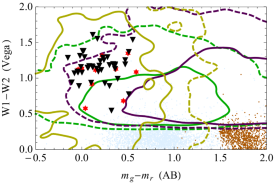
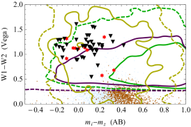
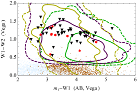
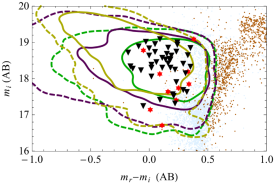
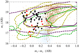
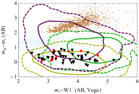
Figure 1 shows these systems in colour-colour space. The need for WISE photometry is evident from the overlap of BC objects with our targets of interest. Also, simple two-colour cuts in SDSS/WISE bands cannot prevent the leakage of BC objects in the quasar locus, whence the necessity of considering nontrivial combinations of bands, which are naturally selected by data mining algorithms.

2.3 Simulated Populations

Figure 2: Example of the systems simulated in this work. Rows 1 and 2: lensed QSOs; rows 3 and 4: a QSO+LRG alignment, rows 5 and 6: a QSO+QSO alignment; rows 7 and 8: a single (isolated, not-lensed) QSO. Bands are $griz$ from left to right, the last sub-panel in each sequence is a $gri$ composite.

In order to reproduce the populations of systems that are expected in a survey, we need to draw the quasars and galaxies from a distribution in redshift and intrinsic properties. We adhere to the common choices for QSO and LRG distributions, as reviewed by OM10, who also used them to generate a mock population of lensed quasars. In particular:

$$n_{gal}(\sigma,z_{g})\mathrm{d}\sigma\mathrm{d}z_{g}\propto(\sigma/\sigma_{\star}(z_{g}))^{\alpha}\exp[-(\sigma/\sigma_{\star}(z_{g}))^{\beta}]\mathrm{d}z_{g}\mathrm{d}\sigma/\sigma$$ (1)

$$n_{qso}(m_{i,q},z_{q})\mathrm{d}m_{i,q}\mathrm{d}z_{q}\propto\frac{10^{-0.4(\alpha+1)(M_{i}-M_{\star}(z_{q}))}}{1+10^{0.4(\beta-\alpha)(M_{i}-M_{\star}(z_{q}))}}\mathrm{d}m_{i,q}\mathrm{d}z_{q}$$ (2)

(parameters further discussed in OM10), where $M_{i}$ is the $i-$band magnitude that the QSO would have at $z_{q}=2$ as computed by Richards et al. (2006). For the population of lensed quasars, we directly use the mock catalogue created by OM10. This provides, for each system: the redshift $z_{g},$ velocity dispersion $\sigma_{g},$ axis ratio and position angle of the lensing galaxy; and the redshift $z_{q},$ unlensed $i-$band magnitude $m_{i,q},$ image positions (relative to the lens) and magnifications of the source quasar. The observables $z_{g},z_{q},\sigma,m_{i}$ and their distributions (eq. 1, 2) can be used also for the $QSO+LRG$ and $2QSO$ simulated classes.

When generating mock observations of these systems, one needs a procedure to prescribe fluxes in different bands, for both the QSO and LRG, and the effective radius of the LRG. The primary observables $\mathbf{p}=(z_{q},z_{g},m_{i,q},\sigma_{g})$ are at our disposal, either drawn from equations (1,2) or from the mock sample of OM10. The remaining observables $\mathbf{r}$ must be matched to those, taking account of intrinsic scatter in those properties (see Mitchell et al., 2005, for the role of scatter in population properties). In other words, if the entries of $\mathbf{p}$ are given, then $\mathbf{r}$ must be drawn from a conditional distribution $\theta(\mathbf{r}|\mathbf{p}).$ The detailed procedure is described in the Appendix, here we summarize its main steps. First, we assemble a sample of LRGs and QSOs, with all the relevant observables, from SDSS and WISE. Then, once values of $\mathbf{p}$ are assigned, a sparse interpolation procedure allows us to build a smooth $\theta(\mathbf{r}|\mathbf{p})$ from the objects within the sample in the vicinity of $\mathbf{p}.$ This way, every time the primary observables are assigned, we can properly draw the other observables within the whole range of LRGs that match $z_{g}$ and $\sigma$, and QSOs that match $z_{q}$ and $m_{i}$.

Within the simulated data sets, we retain just those systems that are brighter than the survey limit ($i-$band magnitude brighter than 21) and with signal-to-noise ratio at least $5,$ which helps prune extreme fluctuations in the simulated sky noise. The cutouts are not necessarily aligned with the p.a. of the image, which forces the learners to concentrate just on those features that are intrinsic to the systems and physically relevant. For the same reason, they are slightly off-centered in different bands – by at most two pixels, a common situation that occurs when downloading image cutouts. We emphasize that the populations simulated here are more general than the SQLS dataset, which relied on a heavy (albeit convenient) selection bias. This point will be discussed further. Some examples of simulated cutouts are shown in Figure 2.

3 Data mining

symbol	meaning
$p$	number of features per object
$K$	number of classes of objects
$\mathbf{f}$	feature vector (in $\mathbb{R}^{p}$)
$\mathbf{y}$	membership probability vector (in $\mathbb{R}^{K}$)
$N_{t}$	objects in a training set
$N_{v}$	objects in a validating set
$R_{err}$	error loss function
$R_{dev}$	deviance loss function
$R_{reg}$	regularization
$M$	number of hidden nodes (in ANNs)
$\lambda$	regularization parameter (in ANNs)

Table 3: Nomenclature used here for our machine-learning techniques (Section 3.4).

In a supervised clasification problem, one is given a training set of $N_{t}$ objects, each of which has a probability vector whose entries are the probabilities of belonging to certain classes. The aim is then to find a best fit to the probability vectors in the training set, together with predictive power on other, new objects. Many techniques have been developed for machine learning and classification (see Ball & Brunner, 2010, for a general review). We will briefly introduce two of them, Artificial Neural Networks (ANNs) and Gradient-Boosted Trees (GBTs), whose choice reflects just our personal preference (see also Section 4.2.2).

In the lens detection problem we train these learners on simulated lensed quasars. Their theoretical performance is evaluated on error and deviance metrics, described in Section 3.3. On the other hand, the searches for lensed quasars are often biased to bright objects with QSO-like photometry, which are not a complete representation of the whole population (c.f. Figure 1). Then, we also evaluate the performance of the learners by testing them against a sample of objects found in past searches, such as the SQLS candidates. In particular, we will test our alogithms on the SQLS morphologically selected sample of lensed QSO targets from SDSS DR7 by Inada et al. (2012).

Regardless of the technique, however, a preliminary step of dimensional reduction on the data is necessary. If we examine 10-arcsecond wide cutouts in $griz$ bands, then each source has a $25\times 25$ image for $g,r,i,$ and $z$, implying a feature space of 2500 dimensions for the raw pixel values. This curse of dimensionality presents a computational challenge, while also leading to an increase in variance and degraded classifier performance. Fortunately, there is significant structure in the images, so that the information can be compressed onto a lower-dimensional manifold. Instead of using the raw data themselves, we first identify features. Some of them are available at catalogue level and reflect some rough physical intuition about the photometry and morphology of the systems, others are data driven, i.e. can be extracted by suitable combinations of pixel values from the cutouts without imposing any physical intuition. This simply generalizes the common procedure of drawing cuts and wedges in colour-magnitude space, in which case the feature array $\mathbf{f}\in\mathbb{R}^{p}$ would simply contain the magnitudes in different bands. Given our mining strategy, we first apply techniques with features extracted from the survey catalogue, then we use data-driven features and pattern recognition on the cutouts of those systems that pass the first selection stage.

Different populations of objects can be separated by setting boundaries in feature space. The accuracy of the classification depends on how many boundaries are set and how flexible they are. The simplest separation relies on linear and affine boundaries, i.e. the partition of feature space ($\mathbf{f}\in\mathbb{R}^{p}$) in regions delimited by hyperplanes, each with weight vector $\boldsymbol{\alpha}$ and bias $a_{0}:$

$$\boldsymbol{\alpha}\cdot\mathbf{f}+a_{0}=0\ .$$ (3)

If different populations overlap in feature space, drawing many boundaries enables the construction of membership probabilities. Finally, a concatenation of classification steps enables the construction of non-linear classifiers. The details of these procedures are specific to different machine learning algorithms.

3.1 Dimensional reduction: catalogue parameters

Figure 3: Correlations among the projections of the simulated cutouts onto some of the first kernel-PCs. Contours delimit the various simulated populations: lensed QSO (green), QSO+LRG (purple), 2QSO (yellow) and single QSOs (blue). The label $\mathrm{KPC}j$ denotes the $j-$th kernel principal component. The populations extend in different directions and partially overlap in kernel-PC space. The separation into classes is attained by modelling the first 200 kernel-PCs simultaneously.

When skimming a whole catalogue for targets, we generalize the SQLS idea of searching for objects with promising photometry and morphological information. In this work, we exploit the magnitudes in $griz$ bands (AB system) and WISE $W1,W2$ bands (Vega system) for the photometric information. The morphology is encoded via the second moments, and from these, the axis ratios and position angles (p.a.s) in the four $griz$ bands. The underlying idea is that the quasar images and the lensing galaxy, when blended together, will still have some distinctive features in the morphology and in how it varies with observing band. For example, in the case of a double we may expect the red deflector to be in the middle and be more relevant in the redder bands. Therefore the elongation should decrease with wavelength, barring uncertainties from noise and pixel-size. Since one p.a. is arbitrary, we use the three differences $(\delta{\phi}_{r},\delta{\phi}_{i},\delta{\phi}_{z})$ between the p.a. in $g$ band and those in the other ones. In the end, this leaves us with $p=13$ features per object, thus mapping the highly dimensional space of raw pixels onto a 13-dimensional feature space.

3.2 Dimensionality reduction: Kernel PCA

Once the targets have been identified in catalog space, we can return to the image pixels and extract more features beyond the simple photo-morphological information used in the previous step. A number of techniques can be deployed to extract data-driven features from the raw pixels in the image cutouts.

We investigated both principal component analysis (PCA) and kernel principal component analysis (KPCA, Schölkopf et al., 1998) on 25 by 25 pixel cutout images. In PCA, the feature vectors are expressed as combinations of the eigenvectors of the data covariance matrix. This is useful in order to isolate the directions of maximum variance and set simple boundaries in feature space. KPCA is similar to PCA, but it uses a kernel $k$ and a map $\Phi$ to embed the feature space $\mathbb{R}^{p}$ into a higher-dimensional space $\mathcal{H},$ such that

$$k(\mathbf{x},\mathbf{y})=\langle\Phi(\mathbf{x}),\Phi(\mathbf{y})\rangle$$ (4)

is a scalar product in $\mathcal{H},$ and then perform the PCA there. There is no need to compute the map $\Phi:\mathbb{R}^{p}\rightarrow\mathbb{R}^{D}$ explicitly – a fact known in jargon as kernel trick. Because of this, KPCA can perform non-linear dimension reduction, while PCA is a linear dimension reduction technique. Further details on KPCA are given in the Appendix and can be found in Schölkopf et al. (1998).

For PCA, we found that the first 500 principal components contain about $90\%$ of the variance in the raw pixel feature space. We can further reduce the number of components by means of the kernel trick. To this aim we used the radial basis function kernel,

$$k(\mathbf{x},\mathbf{y})\ \propto\ \exp\left[-||\mathbf{x}-\mathbf{y}||^{2}/(2\delta^{2})\right]$$ (5)

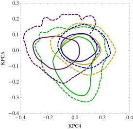
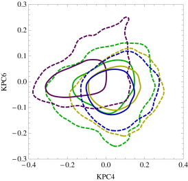
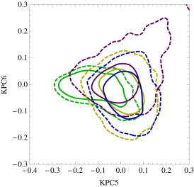
in the 2500-dimensional feature space. The width $\delta$ of the kernel is a tuning parameter. We experimented with a few different values of the kernel width, and found that a value of 0.25 times the median nearest-neighbour distance gave good separation of the classes, as projected onto the first several KPCs. We did not tune this parameter further, choosing rather to use our degrees of freedom for tuning the classifiers as described below. For reference, the projections of the data set classes onto some KPCs are shown in Figure 3.

3.3 Error and Deviance Metrics

In supervised classification, the performance of an algorithm can be quantified by measuring how its output probability vectors $\mathbf{t}_{i}$ deviate from the true ones $\mathbf{y}_{i}$ ($i=1,...,N$ running over a sample of $N$ objects). This can be simply estimated via the error loss function,

$$R_{err}=\frac{1}{N}\sum\limits_{i=1}^{N}||\mathbf{y}_{i}-\mathbf{t}_{i}||^{2}\ .$$ (6)

Another commonly used loss function is the deviance, defined as the conditional entropy of the output probabilities with respect to the true ones:

$$R_{dev}\ =-\sum\limits_{i=1}^{N}\sum\limits_{k=1}^{K}y_{i,k}\log(t_{i,k})\$$ (7)

($K$ being the number of distinct classes). The classifier algorithms are trained to minimize either $R_{err}$ or $R_{dev}$ over suitable training and validating sets, as described in Sect. 3.4, 3.5 below. The error and deviance metrics will also be used to assess the reliability of the learners, once they are trained.

3.4 Techniques: Artificial Neural Networks

class	training	validating
l.QSO	245	100
2QSO	150	80
QSO+LRG	265	100
BC	90	75

Table 4: Objects in the training and validation sets for each class. When training the ANNs, the error and deviance metrics are evaluated on ten different validating sets, so as to have a better grasp on sample-to-sample variance.

For target selection, we use Artificial Neural Networks (ANN). In the simplest ANN scheme, given the feature vectors $\mathbf{x}_{i}$ in the test set ($i=1,...,N_{t}$), the probability vectors $\mathbf{y}_{i}\in\mathbb{R}^{k}$ are fit by combinations

$$\mathbf{t}_{i}=\sum\limits_{m=1}^{M}\boldsymbol{\beta}_{m}g(\boldsymbol{\alpha}_{m}\cdot\mathbf{x}_{i}+a_{0,m})$$ (8)

with every weight $\boldsymbol{\beta}_{m}\in\mathbb{R}^{K}$ and $\boldsymbol{\alpha}_{m}\in\mathbb{R}^{p},$ over a layer of $M$ hidden nodes, where $g$ is a smooth activation function such that $g(\pm\infty)=1/2\pm 1/2.$ One further passage is made in order to ensure that the entries of each $\mathbf{t}_{i},$ being membership probabilities, be positive and sum to unity. Appendix B gives a detailed description of the ANN architecture. The ANN is trained to minimize the error metric (eq. 6). The deviance metric (7) is considered in a subsequent stage.

We also create ten validating sets, where $R_{err}$ is computed but not minimized. We use early stopping, i.e. interrupt the training when the mean error on the validating sets stops decreasing. This is commonly interpreted as a symptom that the learner is becoming greedy to imitate the training set, whilst not improving in predicting the classification of objects in the validating set. The number of objects per class in training and validating sets is given in Table 4. The different proportions of objects were adapted so that the machines would learn to correctly recognise most of them, especially the lensed quasars. For this reason, the fraction of lensed quasars is slightly higher than in the SQLS target sample.

To avoid overfitting, a regularization term

$$R_{reg}=\lambda\sum_{m}\left(||\boldsymbol{\alpha}_{m}||^{2}+||\boldsymbol{\beta}_{m}||^{2}+a_{0,m}^{2}\right)$$ (9)

is added to $R_{err}.$ The performance of the ANN will ultimately depend on $M$ and $\lambda$ (see Sect.4.1).

A faster, albeit less accurate, alternative to ANNs are Extreme Learning Machines (ELMs, Huang et al., 2006), where eq. (8) is used directly and just the $\boldsymbol{\beta}$ weights are optimized. The main advantage of ANNs over ELMs is that the latter’s output are not necessarily probability vectors, i.e. they do not always have positive entries summing to unity. This can be troublesome when new objects are considered, since the ELMs could extrapolate the outputs to values well outside the $[0,1]$ range. The amenable property of ANNs to output probability vectors is the main reason why we have preferred them over ELMs for target selection.

3.5 Techniques: Gradient-Boosted Trees

Gradient boosting (Friedman, 2001) is a general machine learning technique that produces a prediction model using an ensemble of weak learners, where a weak learner is a simple predictive model that may only do slightly better than random guessing. The gradient boosting classifier is built up slowly by fitting a sequence of weak learners to minimize a loss function, which for classification is typically chosen to be the deviance (7). The output for the predictive model is the ensemble average of the prediction for each weak learner. At each iteration of the algorithm, a new weak learner is trained on the residuals for the current model, and this weak learner is added to the ensemble with a contribution proportional to a learning rate parameter. The tuning parameters for the gradient boosting algorithm are the learning rate and the number of weak learners in the ensemble. When the learning rate is smaller, the model is built up more slowly and a larger number of weak learners is needed. Smaller learning rates tend to lead to better test error as they build up the model in a more controlled manner, although they lead to longer computations as they require a higher number of learners. Gradient boosting has been found to be powerful and robust in a variety of different prediction problems (e.g., Hastie et al., 2009), and is very slow to overfit. Further details are given in the Appendix, as well as Friedman (2001) and Hastie et al. (2009).

In our case we use shallow decision trees for the weak learners. A decision tree is made up of a set of binary splits that partition the feature space into a set of constant functions. For classification, the output from the tree is the probability that a data point belongs to a given class given the partition of the input feature space that the data point falls into. The aim is to approximate membership probabilities by piecewise-constant functions in regions $R_{j}$ of feature space,

$$t(\mathbf{x})=\sum\limits_{m=1}^{M}\nu\sum\limits_{j=1}^{J}\gamma_{j,m}I(\mathbf{x}\in R_{j})$$ (10)

(see Appendix B.3), over $M$ trees of depth $J.$

Within the context of gradient boosting, the class probabilities are obtained from the average over the ensemble of shallow decision trees via the learning rate $\nu.$ Because of this, the depth of the trees is an additional tuning parameter in this classification model.

In addition, in our analysis we use a stochastic variant of the original gradient boosting algorithm (Friedman, 2002). In stochastic gradient boosting only a random subsample of the training data is used at each iteration to build the decision tree; note that this subsample is randomly chosen at each iteration of the gradient boosting algorithm, and is not constant throughout the algorithm. (Friedman, 2002) found empirically that random subsampling tended to improve the test errors. In addition, we use random subsampling because it enables us to monitor the deviance loss on the subset of the data that is not used in the fit at each iteration. This yields an estimate of the prediction error of the model as a function of the number of trees, and we choose the number of trees to minimize this estimated prediction error. Other tuning parameters are typically chosen using cross-validation.

3.6 Techniques: Cross-validation

Cross-validation is a statistical technique for estimating the prediction error of a model. The basic idea is to divide the training set into $K$ separate subsamples. Then, one subsample is withheld and the model is trained on the remaining $K-1$ subsamples. The prediction error from this model is calculated for the subsample that was withheld from training the model. The procedure is repeated for each of the other $K-1$ subsamples as well, and the cross-validation error is obtained as the average prediction error over the subsamples.

For most applications, the tuning parameters are chosen to minimize the cross-validation error. In addition, cross-validation is often used to choose the number of features to include in a regression or classification model. Finally, it also helps control overfitting, by attempting to find the tuning parameters and feature set that minimize an average out-of-sample prediction error.

Figure 4: The morphologically-selected candidates in SDSS DR7 by Inada et al. (2012).

4 Results

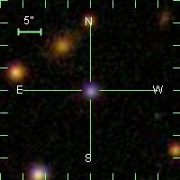
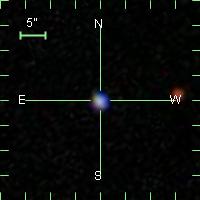
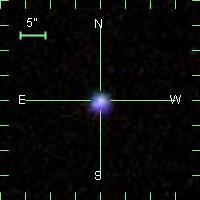
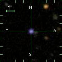
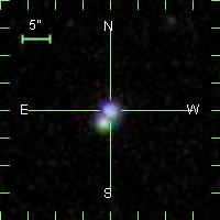
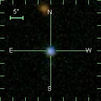
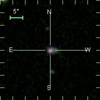
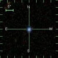
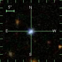
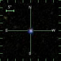
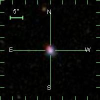
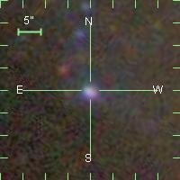
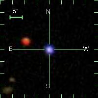
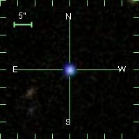
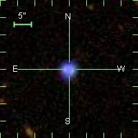
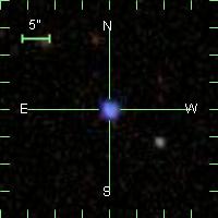
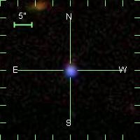
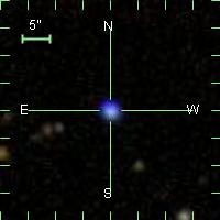
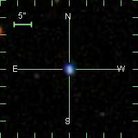
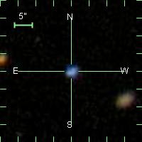
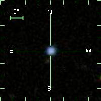
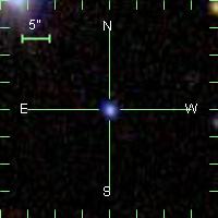
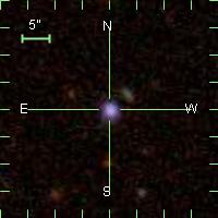
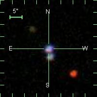
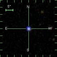
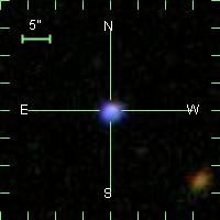
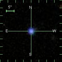
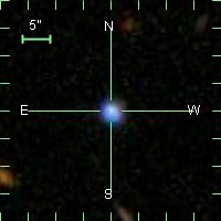
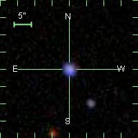
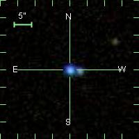
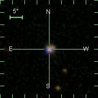
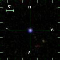
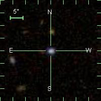
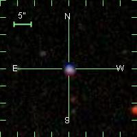
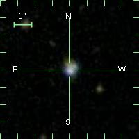
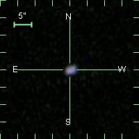
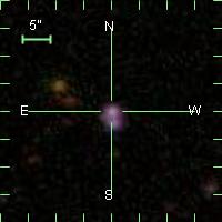
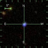
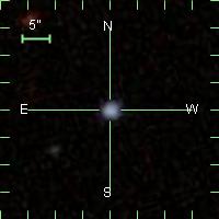
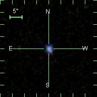
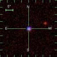
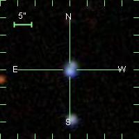
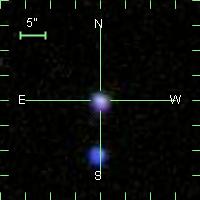
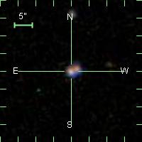
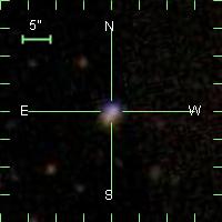
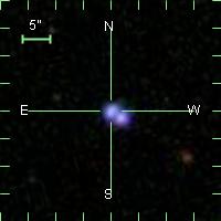
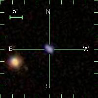
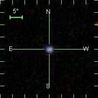
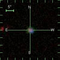
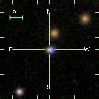
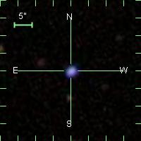
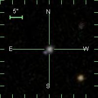
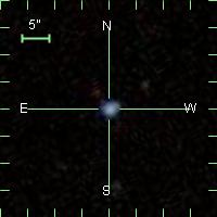
For each of the two steps, target selection and candidate selection, we trained and validated the appropriate learning algorithm from Section 3 using the relevant dataset as defined in Section 2, optimizing their structural parameters by cross-validation. We now quantify the performance of each learner in terms of classification error statistics, deviance, false-vs-true positive rates and purity-vs-completeness, as specified below. Our metrics are built both on the training/validation data, and on the SQLS sample of lensed quasars and false positives (Inada et al., 2012). While examples of the former are displayed in Figure 2, here we show the SQLS objects in Figure 4. Once again, the blended nature and similar colours of the objects are the main obstacles to an efficient and simple separation of true and false positives.

$\lambda$	$M$	$error$	$deviance$	SQLS first test
		per system	per system	purity	completeness
$\lambda=0$	13	$0.56\pm 0.03$	$0.63\pm 0.07$	0.5	0.625
	17	$0.59\pm 0.03$	$0.74\pm 0.09$	0.22	0.225
	20	$0.62\pm 0.04$	$0.69\pm 0.11$	0.30	0.5
	23	$0.56\pm 0.04$	$0.64\pm 0.14$	0.5	0.625
	25	$0.57\pm 0.03$	$0.61\pm 0.09$	0.45	0.625
$\lambda=0.01$	13	$0.61\pm 0.03$	$1.10\pm 0.44$	0.33	0.25
	17	$0.58\pm 0.04$	$0.84\pm 0.36$	0.44	0.5
	20	$0.58\pm 0.04$	$0.94\pm 0.42$	0.475	0.375
	23	$0.57\pm 0.04$	$0.96\pm 0.42$	0.42	0.375
	25	$0.60\pm 0.03$	$0.76\pm 0.10$	0.42	0.62
$\lambda=0.2$	13	$0.56\pm 0.03$	$0.64\pm 0.15$	0.375	0.75
	17	$0.56\pm 0.03$	$0.65\pm 0.15$	0.46	0.75
	20	$0.56\pm 0.03$	$0.64\pm 0.15$	0.4	0.625
	23	$0.56\pm 0.03$	$0.62\pm 0.13$	0.4	0.75
	25	$0.56\pm 0.03$	$0.69\pm 0.20$	0.35	0.625
$\lambda=0.5$	13	$0.57\pm 0.03$	$0.59\pm 0.05$	0.3	1
	17	$0.57\pm 0.03$	$0.59\pm 0.05$	0.3	0.875
	20	$0.57\pm 0.03$	$0.59\pm 0.05$	0.4	0.875
	23	$0.58\pm 0.02$	$0.62\pm 0.04$	0.4	0.875
	25	$0.57\pm 0.02$	$0.59\pm 0.05$	0.35	0.75
$\lambda=1$	13	$0.59\pm 0.02$	$0.65\pm 0.04$	0.3	1
	17	$0.59\pm 0.02$	$0.65\pm 0.04$	0.3	1
	20	$0.59\pm 0.02$	$0.65\pm 0.04$	0.25	1
	23	$0.59\pm 0.02$	$0.65\pm 0.04$	0.30	1
	25	$0.59\pm 0.02$	$0.65\pm 0.04$	0.25	1

Table 5: Performance of the ANNs with different choices of the regularization parameter $\lambda$ and number of nodes $M,$ according to different quantifiers. Columns ‘error’ and ‘deviance’ list the mean loss quantifiers $\sqrt{R_{err}}$ and $R_{dev}$ over the validation set, run on ten different validation sets. The ‘SQLS’ columns list the purity and completeness for the sample of SQLS objects whose output probabilities satisfy $p(QSO+LRG)<0.35,$ $p(BC)<0.35,$ $p(2QSO)<0.8,$ without any further restriction on $p(l.QSO).$

Figure 5: Performance of the target selection, with progressive cuts in the output probabilities, displayed as a receiver operating characteristic curve (top) or purity-completeness plot (bottom). The long-dashed, 1:1 straight line in the bottom panel marks the performance of random classifiers. Grey lines: performance of an ANN with $M=13$ and $\lambda=1$ on the ten validating sets. Other lines mark the performance of the four best ANNs: full (resp short-dashed, dotted, dot-dashed) stands for $M=13$ and $\lambda=1$ (resp. $M=13$ and $\lambda=0.5,$ $M=20$ and $\lambda=0.5,$ $M=20$ and $\lambda=1$). Bullets mark the performance of other ANNs, accepting all objects regardless of $p(l.QSO).$

4.1 Target Selection with Neural Networks

The structural parameters of the ANN we used for lens target selection are the number $M$ of nodes and the regularisation parameter $\lambda.$ We varied $\lambda$ between $0$ and $1,$ whilst $M$ was varied between $13$ and $25.$ The results are shown in Table 5, where the performance is quantified by means of four metrics explained below. These are: rms error and deviance on the validating sets, and purity and completeness when run on the SQLS morphologically selected objects (Inada et al., 2012).

The performance on the validating set is quantified by the classification error and deviance per system. The error per system is defined as the r.m.s. distance of the output probability vectors from their true value, for points in the validating set, i.e. $\sqrt{R_{err}}$ (from eq. 6) for each validating set. Similarly, the deviance per system is $R_{dev}/N_{v}$ (from eq. 7).

When training the ANNs, we followed the behaviour of the error and the deviance on ten different validating sets. This allowed us to assess how the performance of a classifier would vary in practice, if a different validating set were chosen. The values with errorbars in Table 5 then show the average performance on a validating set and its typical (r.m.s.) variability.

The performance on the SQLS objects is measured in terms of the purity and completeness of the selected targets. Alternatively the true- and false-positive rates can be considered, being the fraction of true or false positives that are flagged as possible lensed quasar (l.QSO) targets by the ANNs. For those, one further step is necessary. Since the classifier outputs probabilities for each object to belong to any of the classes, one needs to define a probability threshold in order to select a system as a target or reject it. Objects with $p(QSO+LRG)>0.35,$ $p(BC)>0.35,$ $p(2QSO)>0.8,$ are always flagged as non-targets and rejected. Such a skimming produces a sample of putative lensed QSOs, whose purity and completeness can be used to quantify the efficiency of the ANNs to separate into classes when presented with real data. These are listed in the last column of Table 5.

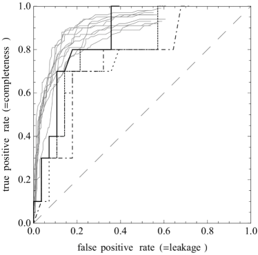
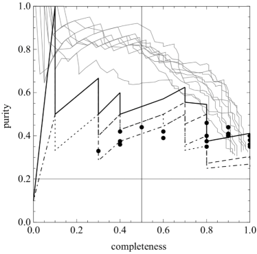
Finally, a minimum threshold must be chosen in order to select just those candidates whose output $p(l.QSO)$ is sufficiently high. By varying the acceptance probability threshold, we can increase the purity of the target set at the expense of completeness – or vice versa. Figure 5 shows the receiver operating characteristic (ROC), i.e. the relation between true positive rate and false positive rate as the acceptance threshold on $p(l.QSO)$ is varied. This figure also shows a plot of purity versus completeness. The black lines display the performance of the best four ANNs (cf Table 5) on the SQLS test objects. The bullets mark the performance of all the other ANNs at maximum completeness, i.e. without cuts in $p(l.QSO).$ For illustrative purposes, the ten grey lines in each panel show the performance of an ANN with $M=13$ and $\lambda=0.5$ on the ten validating sets. When plotting these, the weight of lensed quasars in the validating set has been slightly reduced, in order to match the $20\%$ overall fraction of true positives in SQLS and offer a fair comparison.

4.2 Gradient-Boosted Trees and candidate selection

We trained a classifier directly on the pixel-by-pixel values of the images using several different algorithms. The first step in this process was to normalize all of the images such that the sum of their flux values for each pixel over all of the observational bands was equal to unity. This normalization implies that the classifier will focus on the colour-morphological information for each source. Then, we randomly split the set of simulated images into a training and test set, where the test set contained $25\%$ of the sources. The test set was used to provide an estimate of the test error and was set aside until the end of the analysis; it was not used in the dimension reduction step, nor in the training step.

Unbiased simulated sample.
	percentage classified as…
	l.QSO	2QSOs	QSO+ETG	s.QSO
true l.QSO	88.0	6.7	4.9	0.4
true 2QSO	6.1	57.5	7.3	29.1
true QSO+ETG	6.6	5.8	84.7	2.9
true s.QSO	2.4	13.8	3.2	80.6
Biased simulated sample (eq.s 11).
	percentage classified as…
	l.QSO	2QSOs	QSO+ETG	s.QSO
true l.QSO	84.5	6.5	8.6	0.4
true 2QSO	2.7	84.2	10.9	2.2
true QSO+ETG	6.1	15.3	77.1	1.5
true s.QSO	2.6	59.5	10.3	27.6

Table 6: Confusion matrix for classification of the simulated cutouts with gradient-boosted trees, using KPCA for the dimensional reduction. Top sub-table: unbiased simulated samples; bottom: biased samples following the cuts in eq.s (11).

dim.red.	purity	completeness
PCA (500)	6/8 (=75%)	6/10 (=60%)
KPCA (200)	7/10	7/10 (=70%)

Table 7: Performance of Gradient-Boosted Trees, trained on biased simulated samples, when classifying targets (from Sect.3.4) in the SQLS dataset.

4.2.1 Training and Testing the Gradient-Boosted Decision Trees

We used the stochastic gradient boosting algorithm, with decision tree classifiers as the base weak learners, to train a classifier using the first 200 KPCs derived from the pixel-level information in the images. We set the learning rate to be $\nu=0.01$, a typical value. At each stage we trained the new tree on $80\%$ of the data, while the remaining $20\%$ were used to monitor the validation error. The number of trees in the ensemble were chosen to minimize this validation error, leading to an ensemble of 1190 trees. Since the learning rate is intertwined with the number of trees in the ensemble, there is little to gain from tuning both. The depth of the trees was chosen to minimize the 7-fold cross-validation misclassification error rate, leading to trees with a depth of 5 nodes.

Having exploited much of the photo-morphological information when selecting targets, the classification bottleneck is encountered at this stage. Also, there is a clear selection bias in the SQLS sample, towards objects whose photometry resembles closely that of bright quasars or quasar pairs, as is evident from fig.1. To account for that, we trained the classifiers on cutouts of simulated objects whose photometry satisfied the following, common cuts in colour-magnitude space:

$$16<i<20,\ g-r<0.6,\ r-i<0.45,\ i-z<0.4,$$

$$2.5<i-W1<5,\ 0.5<W1-W2<1.5,$$

$$g-i<1.2(i-W1)-2.8\ .$$ (11)

Table 6 shows the confusion matrix, i.e. the percentage of systems in each class that are either classified correctly (along the diagonal) or as objects of other classes (off-diagonal entries). For the sake of completeness, we list the results both for an unbiased sample and one biased according to eq. (11). The recognition of lensed quasars and quasar pairs does not vary appreciably, the main difference being the misclassification of bright single quasars as possible quasar pairs.

To quantify the performance of the classifiers on the SQLS, we considered just those objects that are flagged as targets from the ANNs (Sect.3.4), since in a realistic search those are the systems that would be inspected with pixel-by-pixel techniques. The results are summarised in Table 7. The importance of PCA versus KPCA is secondary, although the GBTs trained on KPCA use a smaller number of components and produce smoother classification probabilities, which are then more reliable for prediction purposes.

4.2.2 Other Classification Models

We also investigated using the first 500 PCs instead of the first 200 KPCs, but the KPCs sill gave better accuracy. In addition, we also investigated the performance of logistic regression, a single deep decision tree, support vector machines, random forests, and neural networks for classification using the first 200 KPCs. As with the gradient boosted decision tree classifier, the tuning parameters for each classifier were chosen with cross-validation, with the exception of the neural network. We chose the tuning parameters of neural network after some initial exploration and employed early stopping with a validating set of $25\%$ of the training data. Although gradient boosting gave the best performance, the theoretical performance of support vector machines, random forests, and neural networks were all comparable to that.

5 Extensions to other regimes

The choices made in the previous sections are not unique. For example, the target selection can be trained on selected samples as done for the candidate selection, although this does not bring to substantial differences in the performance of the learners. Also, the same techniques can be used to select targets in the deblended regime. For the sake of completeness, in this Section we briefly discuss extensions of our techniques to those two aspects.

5.1 Selection bias

Figure 6: Exploration of the ELMs performance on training and validating sets as a function of nodes. Full black lines: test-set error; grey stripes: average and dispersion of the validating-set error within $1\sigma.$ Top (resp.bottom) panels show the performance of ELMs on the $griz+W1+W2$ bands (resp.adding the second moments), without (left) or with (right) a heavy selection bias towards objects with the photometry of bright quasars. Axes cross at the best validation-set error and at the number of nodes that is required to attain it.

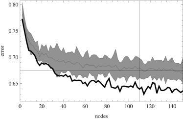
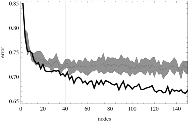
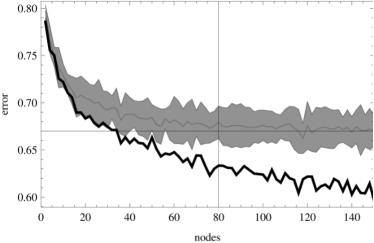
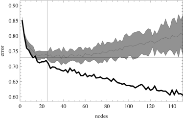
The simplest searches for lensed targets exploit magnification bias, since the brightest objects in a population are likely lensed. On the other hand, this way just the stretched, bright tail of the QSO population is considered, which is not representative of most of the lensed quasars in a survey. Such an effect must be accounted for when tailoring the data mining techniques to a particular survey, such as the SQLS, which can be strongly biased. In the next Section, we will do so ex post by suitably interpreting the membership probabilities that are predicted by the learners, where this is possible. Here, we illustrate the effect of a strong selection bias on the theoretical performance and demands of the learners.

We have simulated different sets of objects, retaining just those systems that satisfy the cuts of eq. 11. For exploratory purposes, we have simply relied on a set of ELMs (Sect. 3.4) to train the target selection. We varied the number of nodes $M$ between 2 and 150. For each choice of $M,$ we have drawn random values of the hidden weights $\boldsymbol{\alpha}$ a hundred times, solved for the output weights $\boldsymbol{\beta}$ on the test set for each of those realizations, evaluated $R_{err}$ on five validation sets and selected just the $(\boldsymbol{\alpha},\boldsymbol{\beta})$ that minimize the average error, which simply defined as $\sqrt{R_{err}}$ on every validation set. This mimics the early stopping criterion of ANNs, while training just on the output weights. The features are standardised and the entries of each $\boldsymbol{\alpha}$ are of the kind $\alpha_{m,l}=\arcsin^{3}(u),$ where $u$ is drawn uniformly in $[0,1].$ This ensures that most of the separating hyperplanes in feature space pass through the bulk of the dataset, while also covering the tails of the distribution.

The results are shown in Figure 6, in four cases: test and validation sets drawn as in the rest of this work or with a heavier selection bias in optical/IR bands (equation 11), considering just the magnitudes ($p=6$ features per object) or also the second moments ($p=13$). If a dataset is unbiased, it offers a complete description of a population, so that most objects will occupy different regions of feature space and the classifiers manage to separate most of them, which is reflected in the smaller validation-set error for the unbiased simulated sample. On the other hand, learners that are trained on heavily biased samples are tailored on simple and lean catalog searches, where they can repay their modest theoretical performance. The information carried by the morphological parameters is not always useful to the learners, especially in the biased case. In fact, the average distance between objects increases rapidly as the dimensionality of feature space is increased, making the data sets too sparse and stretching the differences between objects in the training and validating sets to fictitious levels.

5.2 Larger separations or better image quality

Figure 7: Simulated systems in the deblended regime, with dark green (resp.yellow, dark red) representing l.QSO (resp. 2QSO, ndd) objects. Top: $g-i$ and $i-W1$ colours of the brightest QSO image. Middle: output $p(l.QSO)$ versus $i-W1$ colour of the bright image. Bottom: output $p(l.QSO)$ versus half of the image-separation in arcseconds. A depth $i=24.0$ and PSF FWHM$=0.85^{\prime\prime}$ have been adopted here.

Figure 8: ROC plots for target selection in the deblended regime. The grey lines show the performance on the five validating sets when just $l.QSO$ systems are considered as true positives. The black lines refer to the selection of both $l.QSO$ and $nlo$ systems. As $nlo$ systems have a faint deflector, they are mostly classified as QSO pairs.

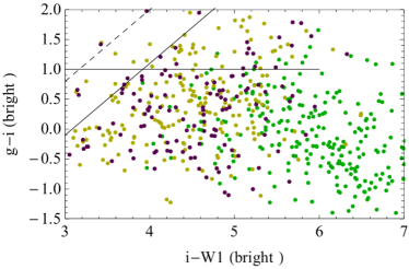
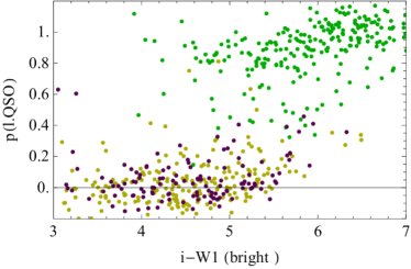
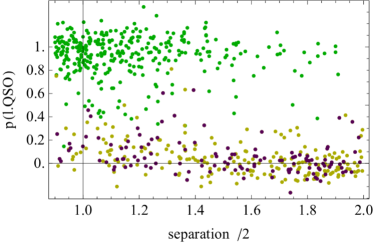
Depending on the image separation and imaging quality of a survey, an appreciable fraction of lensed quasars can appear as close ($\theta_{sep}\leq 4^{\prime\prime}$) QSO pairs. This can be the case, for example, with the claimed depth ($i\approx 24$) and image quality (median FWHM$\approx 0.85$) of DES and will be even dominant for Gaia (resolution $\approx 0.15^{\prime\prime}$). Here we illustrate how the same techniques, specifically ELMs (Sect.s 3.4, B.2), can be used to study the search for lensed quasars in the deblended regime.

We have simulated two classes of objects, lensed quasars (l.QSO) and line-of-sight quasar pairs (2QSO), with the same procedures as for the blended case, plus a third class that will be described below. As the fainter image of a lensed QSO is also closer to the deflector, one must add a differential reddening between multiple images, since colour comparison is a criterion for colour selection of close-by, quasar-like objects. We refer to Oguri et al. (2006) for more detail on the acceptable region for the reddening vector in $griz$ bands. Also, the PSF-photometry and morphology of the faintest QSO image are more contaminated by the deflector’s flux. Still, we can safely suppose that the QSO images will not appear as extended, as is confirmed in practice by previous searches.

For these reasons, the data mining in the deblended regime is trained on the following features: PSF magnitudes in $griz$ of the images; overall $W1,W2$ magnitudes; flattening and position angle of the faint image in $griz$ bands; and faint-to-bright image position angle. When simulating l.QSO systems, we compare the overall $i-$band magnitude of the simulated cutout with the global PSF magnitudes of the QSO images to estimate the mean surface-brightness $SB(R_{E})$ of the deflector within the Einstein radius. The distribution of $SB(R_{E})$ shows a secondary peak beyond $\approx 18.5,$ so if a simulated object has $SB(R_{E})>18.5,$ we store it in a third class (ndd, no detected deflector).

The results of this procedure are displayed in Figure 7, for the test set only for visual convenience. We have chosen the half-separation in the last panel because that is also a rough estimate of the Einstein radius for the $l.QSO$ systems. If the $g-i$ and $i-W1$ colours of the bright QSO image are considered, regardless of the class, the $i-W1$ colour is larger than in equation 11, simply because the $W1$ magnitude encloses the flux from the whole system, because of the large WISE FWHM. The full lines in the top panel show the colour cuts as in eq. (11), the dashed line is simply shifted by $1.2\times 2.5\log_{10}(2)\approx 0.9,$ as would be expected in a QSO pair with comparable $i-$band fluxes between the two objects. The middle panel shows the output $p(l.QSO)$ as a function of bright image $i-W1,$ whereas in the bottom panel $p(l.QSO)$ is examined against the image separation. It becomes evident that, even if 2QSO systems become more frequent and dominate at larger separations, data mining on the photo-morphological features is still effective at separating the classes, except for those few systems where the deflector is not bright enough – as exemplified by the ndd systems, which are unrecognised lensed quasars.

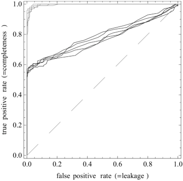
A more quantitative analysis is shown in the ROC plots of Figure 8 on the validating sets. If just $l.QSO$ systems are our main interest (grey curves), the performance in excellent. The recovery of both $l.QSO$ and $nlo$ systems (i.e. regardless of the deflector’s brightness, black curves) is less sharp, as $nlo$ systems are mostly classified as $2QSO.$

6 Conclusions

We have applied machine-learning techniques to the search for gravitationally lensed quasars in wide field imaging surveys, breaking down the problem into two stages, target selection and candidate selection. In the target selection stage, promising systems were selected based solely on information available at the catalogue level. Focusing on SDSS and WISE data, in order to compare with the actual output of the SDSS Quasar Lens Search, we used thirteen parameters: the magnitudes in $griz$ and WISE $W1,W2$ bands, and the axis ratios and position angles in the SDSS $griz$ bands. In the candidate selection stage, we returned to the images of the targets in order to narrow down the search: we used 10 arcsecond ($25\times 25$ pixel) SDSS cutout images in $griz$, and reduced the dimensionality of the feature space (from 2500 to 200) via kernel-PCA.

In order to have a large set of objects, for training and validation we used a mixture of simulated and real objects, all assuming or directly sampling the SDSS imaging conditions. In particular, we simulated systems in three classes (lensed QSO, QSO+LRG alignment, QSO+QSO alignment), and added a sample of Blue Cloud (BC) galaxies drawn from SDSS. For the candidate selection stage, we discarded the BC galaxies and included a simulated sample of single quasars. This allowed us to explore the range of true- and false-positives in a strategy that might be followed in an SDSS lensed quasar search restricted not to use any spectroscopic information.

Artificial Neural Networks were used to separate lensed quasar targets from false positives. In particular, we focused on single-hidden layer, feed-forward networks, which are trained with backpropagation and early stopping. The use of such ANNs on the photo-morphological features enables the separation of QSO-like objects from Blue-Cloud galaxies, which would otherwise be a dominant source of contamination for samples of extended objects selected in $griz+W1+W2$ bands. In particular, with hard cuts in optical/IR bands (eq.11) and the requirement of extended morphology, about a tenth of the Blue Cloud galaxies leak into the sample of targets with extended morphology brighter than 19 in $i-$band. Use of ANNs prunes these away effectively, reducing the leakage to the percent level. When tested on the SQLS morphologically-selected sample, which is biased towards bright quasars, the best ANNs give a twofold (up to threefold) increase in purity at the price of a $10\%$ (or $20\%$) reduction of the completeness.

Returning to the pixels for candidate selection, we trained Gradient-Boosted Trees on the kernel-PCA features extracted from simulated images of plausible targets, whose photometry obeys a selection bias similar to that of SQLS objects (equation 11). When tested on the targets selected by the ANNs, this system gave a final purity of $70\%$ while correctly identifying $70\%$ of the true positives.

In the broader context, our novel technique is highly complementary to and synergistic with alternative approaches that are or have been proposed. For example the ANN catalog level selection, with its high completeness and reasonable purity, could be used to pre-select targets for human classifiers in a citizen science project, or to be fed to robots designed to automatically model the lensing features in pixel space (e.g. Marshall et al., 2009). These approaches could be run in parallel to the kPCA method proposed here, and with each other: in order to find reliably large samples of lensed quasars it is possible that many of these techniques will have to be used in parallel.

A significant advantage of machine learning techniques, like those explored here, is that they are very fast both to train and to run as classifers. Speed will be essential to find large sample of lensed quasars in ongoing and upcoming imaging surveys, such as PS1, DES, HSC, and LSST. Searches in these surveys that use traditional lens finding techniques would require several seconds of CPU or investigator time per system for very large numbers of objects. In contrast, with a run-time of $\approx 10^{-3}$ seconds per system, the machine learning target selection presented here could perform a catalog search over the DES-wide footprint in just a few hours on a 12 core desktop workstation. Assuming conservatively a purity between 20% and 50% from this catalog search, finding the brightest 100 lenses in DES would require running the pixel based algorithm on only a few hundred cutouts, which is a trivial computational task.

As follow-up efforts provide larger and larger samples of false and true positives for each survey, they will provide new training sets to improve algorithms such as these. Furthermore, as data are reprocessed and improved the search can also be repeated with minimal expense. Finally, these techniques are inherently repeatable so that the results can be reproduced by independent users. What deserves further investigation is how well machine classifiers perform when presented with test sets that contain unusual lenses. An example in the present context might be a system with significant differential reddening or microlensing. We do not expect the extension of the methods applied here to larger feature sets to pose significant problems: additional information, particularly from the time domain (e.g. Schmidt et al., 2010) would be straightforward to include. Including catalog variability parameters, or time series of image cutouts, would be an interesting next step.

In conclusion, we have used the SQLS and simulated samples to illustrate the power of machine learning techniques in finding gravitationally lensed quasars. We have illustrated how it works on blended (and hence difficult) objects, but it can be naturally applied also to the deblended regime (Section 5.2). Even though these techniques might seem cumbersome (perhaps even “Rococo”), it is striking how much improvement is afforded over simpler, traditional techniques. For example, the ANN catalog-level search yields a purity up to $\approx 60\%$, which is appreciably better than what was achieved by SQLS and an order of magnitude higher than what can be achieved with simple colour cuts in $griz$+WISE and the requirement of spatial extension. This means reducing the follow-up effort by the same amount, a crucial goal if one wants to confirm large samples of lenses. For example, in order to find of order 100 lensed quasars from a Stage III experiment like DES one would have to follow-up only $\approx$200 candidates, as opposed with the thousands required for purities below 10%. With the addition of time domain information, the methods should further improve their performance in terms of purity, which will be key to containing follow-up costs.

Appendix A Simulated galaxies and quasars

Figure 9: Schema of the empirical matching procedure, in this case for the quasars. The primary observables are binned; the conditional probability $\theta(\mathbf{r}|\mathbf{p})$ is constructed in each bin; when a new system is considered, the conditional distribution of its observables is interpolated among its nearest neighbours in the space of primary observables.

For the simulated systems for this work, we needed the magnitudes of QSOs and LRG in $griz$ and $W1,W2$ bands, the effective radii of the LRGs and a prescription to link those to the primary observables in eq.s (1) and (2). We proceed by assembling a catalogue of QSOs and one of LRGs (spectroscopically-confirmed) from SDSS and WISE. For each of the quasars, we retrieve the redshift $z_{q}$ and apparent magnitudes in $(g,r,i,z,W1,W2)$ optical/IR bands. For each LRG, we retrieve its redshift $z_{g},$ magnitudes in optical/IR bands, velocity dispersion $\sigma$ and $r-$band effective radius $R_{e}.$ Both the QSO and LRG queries are split into redshift bins of width $\delta z=0.1,$ with $10^{3}$ objects in each bin, so as to ensure an even coverage of the redshift range.

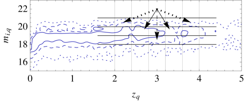
From the SDSS+WISE catalogues we can build the conditional probability $\theta(\mathrm{r}|\mathrm{p})$ that a QSO (resp.LRG) with observables $\mathrm{p}=(z_{q},m_{i})$ (resp. $z_{g},\sigma$) has some values of the remaining observables $\mathrm{r}.$ We first bin the QSO (resp.LRG) catalogue in redshift and $m_{i}$ (resp. $\sigma$), so that in each bin the mean and covariance of the remaining observables can be easily computed. In other words, we have a characterization of the conditional probability at some discrete locations, $\theta(\mathbf{r}|\mathbf{p}_{l})_{l=1,...,N_{bins}}.$ The next step is to build a smooth interpolation of those, across the whole range of redshift and $m_{i}$ (or $\sigma$). This is needed in order to assign values of $\mathbf{r}$ also to systems whose primary observables $\mathbf{p}$ are not well represented by the SDSS+WISE catalogue. Figure 9 summarizes the main steps.

Given a pair $\mathbf{p}=(z_{q},m_{i})$ for a QSO in the simulated catalogue, we find its corresponding bin, say $\mathbf{p}_{n,m}=(z_{q,n},m_{i,m}),$ and build a sparse interpolation for $\theta(\mathbf{r}|\mathbf{p})$ as

$$\theta(\mathbf{r}|\mathbf{p})=\frac{\sum\limits_{i,j}\theta(\mathbf{r}|\mathbf{p}_{i,j})\exp[-|i-n|-|j-m|]}{\sum\limits_{i,j}\exp[-|i-n|-|j-m|]}\ .$$ (12)

The fast exponential fall-off of the weights ensures that just the nearest (populated) neighbour bins give a contribution to the interpolated probability. This is useful in order to smooth out bin-to-bin noise and obtain a smooth probability also for bins that are not well populated. In practice, instead of computing the whole probability distribution in each bin, we compute the mean and dispersions of $\mathrm{r}$ and interpolate those similarly to eq. (12). The procedure is the same for LRGs, with the obvious changes, and allows us to draw magnitudes (and effective radii) that are as close as possible to the ones found in SDSS and WISE.

Figure 10: Composite $gri$ plots of the first 18 principal components of the simulated sample.

Appendix B Dimensional reduction and Machine-learning algorithms

In all of the machine-learning techniques the features are standardized, i.e. we subtract the test-set average and divide by the variance. This way, we operate on feature vectors with entries typically within $[-1,1],$ overcoming issues related to the choice of units of measure and zero-points.

B.1 PCA and kPCA

When separating objects in different classes, we tacitly suppose that their features are linked to one another through relations that, in general, must be found. In other words, the data features are usually correlated and we may seek new combinations of features that naturally follow these correlations. In Principal Component Analysis (PCA), a training set of vectors $\left\{\mathbf{x}_{i}\right\}_{i=1,...,N}$ is linearly transformed into a set $\left\{\mathbf{f}_{i}\right\}_{i=1,...,N}$ whose new features are uncorrelated, i.e. $\langle f_{n}f_{m}\rangle=(1/N)\sum_{i}f_{i,n}f_{i,m}=0.$ This is simply achieved by diagonalizing the data covariance matrix $C_{n,m}=\langle x_{n}x_{m}\rangle.$ The principal components are the eigenvectors $\mathbf{w}_{1},...,\mathbf{w}_{p}$ of $C_{n,m},$ and the coordinates of a vector $\mathbf{x}_{i}$ in this basis are the projections $t_{i,r}=\mathbf{w}_{r}\cdot\mathbf{x}_{i}.$

The sum

$$var(r)=\frac{\sum_{m=1}^{r}\langle t_{m}^{2}\rangle}{\sum_{m=1}^{p}\langle t_{m}^{2}\rangle}$$ (13)

is the fraction of explained variance within the dataset up to the $r-$th component. Because of this, PCA can also be used to de-noise and reduce the dimensionality of the problem at hand, by retaining just the projections onto the first $r$ components, at the price of encompassing just a fraction $var(r)$ of the whole feature variability.

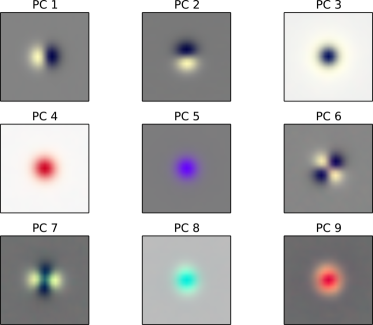
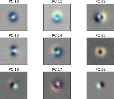
In our case, each feature vector consists of four concatenated $25\times 25$ pixel cutouts, one per band, normalized to the total flux. Hence, the principal components are combinations of shapelet images in the four $griz$ bands. Figure 10 shows $gri$ composites of the first $18$ principal components for our training set of simulated cutouts.

Kernel Principal Component Analysis (kPCA, Schölkopf et al., 1998) provides a very elegant extention of the PCA approach, by supposing that the feature space is a (perhaps unfortunate) projection of a $p-$dimensional manifold which resides in a higher-dimensional feature space. In fact, in PCA-based classification one relies just on the coordinates $t_{i,r}=\mathbf{w}_{r}\cdot\mathbf{x}_{i}$ rather than the principal component vectors themselves. Within kPCA, the scalar product $\mathbf{x}\cdot\mathbf{w}$ in $\mathbb{R}^{p}$ is replaced with a semi-positive definite kernel $k:\mathbb{R}^{p}\times\mathbb{R}^{p}\rightarrow\mathbb{R},$ provided there is a nonlinear map $\Phi:\mathbb{R}^{p}\rightarrow\mathcal{H}$ onto a higher-dimensional Hilbert space, such that $k(\mathbf{x},\mathbf{y})=\langle\Phi(\mathbf{x}),\Phi(\mathbf{y})\rangle$ is a scalar product in $\mathcal{H}.$ Now the task it so diagonalize the new covariance matrix operator in $\mathcal{H}$

$$\tilde{\mathrm{C}}=\frac{1}{N}\sum\limits_{i=1}^{N}\Phi(\mathbf{x}_{i})\Phi(\mathbf{x}_{i})^{{\dagger}}$$ (14)

The eigenvectors $\mathbf{v}_{r}$ of $\tilde{\mathrm{C}}$ must be linear combinations of the new feature vectors in $\mathcal{H},$

$$\mathbf{v}_{r}=\sum\limits_{i=1}^{N}a_{r,i}\Phi(\mathbf{x_{i}})\ ,$$ (15)

which gives a new eigenvalue equation for $K_{i,j}=(1/N)\langle\Phi(\mathbf{x}_{i}),\Phi(\mathbf{x}_{j})\rangle\equiv(1/N)k(\mathbf{x}_{i},\mathbf{x}_{j})$ and the weights $a_{j,i}$

$$\mathrm{K}\mathbf{a}=\lambda\mathbf{a}\ .$$ (16)

Once the (orthonormal) weight vectors $a_{r,i}$ are found, the kPCA components in $\mathcal{H}$ of a feature vector $\mathbf{f}\in\mathbb{R}^{p}$ are simply

$$\tilde{t}_{r}=\ \langle\mathbf{v}_{r},\Phi(\mathbf{f})\rangle=\sum\limits_{i=1}^{N}a_{r,i}\langle\Phi(\mathbf{x}_{i}),\Phi(\mathbf{f})\rangle\ =\ \sum\limits_{i=1}^{N}a_{r,i}k(\mathbf{x}_{i},\mathbf{f})\ .$$ (17)

A suitable adaptation of Mercer’s theorem (Ferreira and Menegatto, 2009) ensures that $\Phi$ exists whenever $k$ is semi-positive definite, however it will generally map $\mathbb{R}^{p}$ into an infinite-dimensional Hilbert space. Fortunately, since just the kPCA components are used for classification, we never need to compute the map $\Phi$ explicitly and the non-linear structure of the data is simply encoded in the kernel $k$ via eq.(17).

B.2 Artificial Neural Networks and Extreme Learning Machines

Let us consider a smooth, increasing activation function $g:\mathbb{R}\rightarrow\mathbb{R}$ such that

$$\lim\limits_{x\rightarrow+\infty}g(x)=1\ ,\ \lim\limits_{x\rightarrow-\infty}g(x)=0\ .$$ (18)

The idea underlying ANNs is to use $g$ to construct arbitrarily good approximations to given functions over the feature space $\mathbf{x}\in\mathbb{R}^{p}.$ In particular, any piecewise continuous function $g:\mathbb{R}^{p}\rightarrow\mathbb{R},$ defined on a compact subset of $\mathbb{R}^{p},$ can be approximated by combinations of the kind

$$t=\sum\limits_{m=1}^{M}\beta_{m}g(\boldsymbol{\alpha}_{m}\cdot\mathbf{x}+a_{0,m})\ .$$ (19)

The number of nodes M depends just on the tolerance that is desired in order to fit $y.$ The same holds, quite naturally, for multidimensional (piecewise continuous) functions $\mathbf{y}=(y_{1},...,y_{K}),$ mapping a compact subset of $\mathbb{R}^{p}$ into $\mathbb{R}^{K}.$ This is the case of classification problems, where $\mathbf{y}$ gives the membership probabilities to different classes for an object in feature space. A common choice for the activation function is the sigmoid $g(x)=1/(1+\mathrm{e}^{-x}).$

Approximations as in eq.(20) are the core of Extreme Learning Machines (ELMs, Huang et al., 2006), where the weights and biases $(\boldsymbol{\alpha}_{m},a_{0,m})$ are held fixed and the parameters $\beta_{m}$ are adjusted. Specifically, operating a test set $\left\{\mathbf{x}_{i}\right\}_{i=1,...,N_{t}}$ with probability vectors $\left\{\mathbf{y}_{i}\right\}_{i=1,...,N_{t}},$ the weights $\boldsymbol{\beta}_{m}$ can be found as:

$$\boldsymbol{\beta}_{m}=W^{{\dagger}}_{i,m}\mathbf{y}_{i}\ ,$$ (20)

where $W^{{\dagger}}$ is the pseudo-inverse of a matrix $W$ with entries $W_{i,j}=g(\boldsymbol{\alpha}_{j}\cdot\mathbf{j}+a_{0,j}).$ We can also add a constant vector $\beta_{0}$ in the approximation $\mathbf{t}$, which is equivalent to having (at least) one of the activation functions $g(\boldsymbol{\alpha}_{j}\cdot\mathbf{x}+a_{0,j})$ equal to one. Similarly, we can regard the coefficients $a_{m,0}$ as part of the weight vectors $\boldsymbol{\alpha}_{m},$ if we embed $\mathbb{R}^{p}$ in $\mathbb{R}^{p+1}$ as $(x_{1},...,x_{p})\mapsto(x_{1},...,x_{p},1).$ This is the convention that we will adopt in what follows.

The approximating solutions $\mathbf{t}(\mathbf{x})=(t_{1},...,t_{k})$ from ELMs are not necessarily probability vectors, which are required to have positive entries that sum to unity. Hence, when using ANNs for classification a final transformation $t_{k}\mapsto g_{k}(\mathbf{t})$ is made, with $g_{k}$ commonly chosen as the soft-max

$$g_{k}(\mathbf{t})=\frac{\exp[t_{k}]}{\exp[t_{1}]+...+\exp[t_{K}]}\ .$$ (21)

The ANNs are trained by minimizing a loss function, wich can be either $R_{err}+R_{reg}$ or $R_{dev}+R_{reg},$ which can be simply implemented by means of steepest descent methods since the derivatives with respect to the weights $(\boldsymbol{\beta},\boldsymbol{\alpha})$ can be computed analytically:

$$R_{err}=\frac{1}{N}\sum_{i,k}(y_{i,k}-g_{k}(\mathbf{t}_{i}))^{2}\ \equiv\ \frac{1}{N}\sum_{i}R_{i}$$ (22)

$$\partial_{\beta_{m,k}}R_{i}=\frac{2}{N}(g_{k}(\mathbf{t}_{i})-y_{i,k})g^{\prime}_{k}(\mathbf{t}_{i})g(\boldsymbol{\alpha}_{m}\cdot\mathbf{x}_{i})\ \equiv\ \delta_{k,i}g(\boldsymbol{\alpha}_{m}\cdot\mathbf{x}_{i})$$ (23)

$$\partial_{\alpha_{m,l}}R_{i}=\sum\limits_{k=1}^{K}\frac{2}{N}(g_{k}(\mathbf{t}_{i})-y_{i,k})g^{\prime}_{k}(\mathbf{t}_{i})\beta_{k,m}g^{\prime}(\boldsymbol{\alpha}_{m}\cdot\mathbf{x}_{i})x_{i,l}\ \equiv\ s_{m,i}x_{l,i}$$ (24)

Given the structure of the ANNs illustrated here, some convenient back-propagation relations hold among the coefficients, which descend from the additive nature of the loss function. For example, when the loss function is just $R_{err},$ one has

$$s_{m,i}=g^{\prime}(\boldsymbol{\alpha}_{m}\cdot\mathbf{x}_{i})\sum_{k=1}^{K}\beta_{k,m}\delta_{k,i}\ .$$ (26)

The gradients and back-propagation relations can be computed also for other choices of the loss function along these lines.

If a large number of nodes is used, or if the coefficients are completely unconstrained, one can overfit peculiar behaviours of observables in the test-set, which are not necessarily present in other datasets, thus losing predictive power. To avoid this, the loss function is also computed on some validating sets, with objects drawn from the same parent distributions as in the test set, and the optimization on the test set is stopped when the error on the validating sets does not decrease any more. For the analysis in Sect.4.1 we have assembled ten validating sets, as to have a characterization of the typical error and its variation over different datasets. The addition of a regularization term has a similar effect. In fact, the classification problem corresponds to mapping the feature space into a classification manifold, parameterized by the membership probabilities $(y_{1},...,y_{K}),$ and regularization helps ensure that new objects will be mapped smoothly on the classification space. Extreme Learning Machines offer an alternative to early stopping and regularization. First, the $\boldsymbol{\beta}$ coefficients from eq.(20) have the smallest possible norm among all those that minimize the test-set error $R_{err},$ a similar outcome to regularization. Second, if a node has $\boldsymbol{\alpha}$ weights that are not well discriminatory, it will automatically have a small $\boldsymbol{\beta}$ coefficient, avoiding the need to back-propagate in $\boldsymbol{\alpha}.$ Third, since $W^{{\dagger}}$ in eq.(20) is computed very fast, one can draw many random combinations of $\alpha$ weights and retain just the $\beta$ solution that minimizes the validation error – it also minimizes the test-set error, by construction.

B.3 Gradient-Boosted Trees

For completeness, we summarize the gradient boosting algorithm for classification using decision trees. Our description follows that of Hastie et al. (2009), to which we refer the reader for further details.

In gradient boosted decision trees the predicted output, $f(x)$, is modeled as a function of the inputs $x$ as a sum of $M$ trees

$$f(x)=\sum_{i=1}^{M}\nu T(x,\Theta_{m}).$$ (27)

The parameter $\nu$ is called the learning rate, and regularizes the model by controlling how much each tree contributes to the sum. A tree is formally expressed as

$$T(x,\Theta)=\sum_{j=1}^{J}\gamma_{j}I(x\in R_{j}),$$ (28)

where $I(\cdot)$ denotes the indicator function that returns 1 if the argument is true, and 0 otherwise. The parameters $\Theta=\{R_{j},\gamma_{j}\}$ represent the partition of the input space and the output for each partition, respectively, and are fit using a training set. The meta-parameter $J$ controls the number of partitions of the input space, and can be estimated through cross-validation, or using a separate validating set. From Equation (28) one sees that a decision tree is a piecewise constant model.

Gradient boosting is an algorithm for minimizing a loss function that is modeled after techniques from numerical optimization. For classification, the functions $f_{k}(x)$ represent the unnormalized log-probability for the $k^{\rm th}$ class. They are related to the class probabilities $p_{k}$ by

$$p_{k}=\frac{\exp(f_{k}(x))}{\sum_{l=1}^{K}\exp(f_{l}(x))}.$$ (29)

When there are more than two classes, gradient boosting fits a separate sum of trees to each class, and com,es them using Equation (29). The training set outputs $y_{1},\ldots,y_{n}$ are integer values representing the class labels, which take values from the set $\{G_{1},\ldots,G_{K}\}$.

The typical loss function for classification problems is the multinomial deviance

$$L(f)=-\sum_{i=1}^{n}\sum_{k=1}^{K}I(y_{i}=G_{k})f_{k}(x_{i})+\sum_{i=1}^{n}\log\left(\sum_{k=1}^{K}e^{f_{k}(x_{i})}\right).$$ (30)

(cf. eq.7). The optimization problem is to find the values of ${\bf f}_{k}=[f_{k}(x_{1}),\ldots,f_{k}(x_{n})]^{T}$ that minimize Equation (30). Note that at this point it is not necessary that the functions $f_{k}(x)$ be a sum of trees. Sequential numerical optimization algorithms would express the solution as a sum of vectors

$$\hat{\bf f}_{kM}=\sum_{m=0}^{M}{\bf h}_{km},$$ (31)

where the first vector ${\bf h}_{k0}$ represent the initial guess, and the remaining $M$ vectors represent the updates as the algorithm evolves. It is common to choose the next vector in the minimization procedure as proportional to the gradient of the loss function, meaning that the algorithm evolves by stepping in the direction of largest negative change in the loss function. For example, using the initial guess ${\bf h}_{k0}$ the estimated function that minimizes the loss function would simply be $\hat{\bf f}_{k0}={\bf h}_{k0}$. We can improve upon this estimate as

$$\hat{\bf f}_{k1}=\hat{\bf f}_{k0}-\rho_{1}{\bf g}_{k1},$$ (32)

where $\rho_{1}$ represents the step size and ${\bf g}_{1}$ is the gradient vector evaluated at $\hat{\bf f}_{k0}$:

$$g_{ik1}= \left.\frac{\partial L(y_{i},f_{k}(x_{i}))}{\partial f_{k}(x_{i})}\right|_{f_{k}(x_{i})=\hat{f}_{k0}(x_{i})}$$

$$= -I(y_{i}=G_{k})+p_{k}(x_{i}).$$ (33)

The step size may be chosen to minimize the loss function $L(\hat{\bf f}_{k1})$. The procedure is repeated $M$ times, leading to Equation (31) where ${\bf h}_{m}=-\rho_{m}{\bf g}_{km}$.

If we were only interested minimizing the loss on the training data, then we have everything we need in Equations (31)–(33). However, we want to generalize our model to make new predictions, so we want to also minimize the loss function with respect to data outside of the training set. We could do this if we had the values of the gradient at other data points as well. The principal idea behind gradient boosting is to fit a tree to the negative gradient at each iteration, which then allows us to generalize the gradient beyond the training set. In this case, the updates ${\bf h}_{km}$ are trees, leading to a solution (Eq. 31) which is a sum of trees (Eq. 27). The learning rate $\nu$ is analogous to the role of the step size $\rho_{m}$, as it controls how fast the optimization algorithm proceeds, and thus how much each tree contributes to the sum. Smaller values of $\nu$ ($\rho_{m}$) lead to better models (optimization solutions), but require more trees (optimization steps).

References

- Abazajian et al. (2009) Abazajian, K. N., Adelman-McCarthy, J. K., Agüeros, M. A., et al. 2009, ApJS, 182, 543
- Ball et al. (2008) Ball, N. M., Brunner, R. J., & Myers, A. D. 2008, Astronomical Data Analysis Software and Systems XVII, 394, 201
- Ball & Brunner (2010) Ball, N. M., & Brunner, R. J. 2010, International Journal of Modern Physics D, 19, 1049
- Blagorodnova et al. (2014) Blagorodnova, N., Koposov, S. E., Wyrzykowski, Ł., Irwin, M., & Walton, N. A. 2014, MNRAS, 442, 327
- Belokurov et al. (2003) Belokurov, V., Evans, N. W., & Du, Y. L. 2003, MNRAS, 341, 1373
- Blackburne et al. (2014) Blackburne, J. A., Kochanek, C. S., Chen, B., Dai, X., & Chartas, G. 2014, ApJ, 789, 125
- Carrasco Kind & Brunner (2014) Carrasco Kind, M., & Brunner, R. J. 2014, MNRAS, 442, 3380
- Courbin et al. (2002) Courbin, F., Saha, P., & Schechter, P. L. 2002, Gravitational Lensing: An Astrophysical Tool, 608, 1
- Dai et al. (2006) Dai, X., Kochanek, C. S., Chartas, G., & Mathur, S. 2006, ApJ, 637, 53
- Dalal & Kochanek (2002) Dalal, N., & Kochanek, C. S. 2002, ApJ, 572, 25
- Ferreira and Menegatto (2009) Ferreira, J. C., Menegatto, V. A. 2009, Integral equation and Operator Theory, 64 no. 1, 61–81.
- Finet et al. (2012) Finet, F., Elyiv, A., & Surdej, J. 2012, MmSAI, 83, 944
- Friedman (2001) Friedman, J. H. 2001, The Annals of Statistics, Volume 29, Issue 5, Pages 1189–1232
- Friedman (2002) Friedman, J. H. 2002, Computational Statistics & Data Analysis, Volume 38, Issue 4,Pages 367–378
- Guerras et al. (2013) Guerras, E., Mediavilla, E., Jimenez-Vicente, J., et al. 2013, ApJ, 764, 160
- Hastie et al. (2009) Hastie, T., Tibshirani, R., and Friedman, J. H. 2009, The elements of statistical learning: data mining, inference and prediction, Springer
- Huang et al. (2006) Huang, G.-B., Zhu, Q.-Y., and Siew, C.-K. 2006, Neurocomputing, vol. 70, pp. 489-501
- Inada et al. (2012) Inada, N., Oguri, M., Shin, M.-S., et al. 2012, AJ, 143, 119
- Inada et al. (2014) Inada, N., Oguri, M., Rusu, C. E., Kayo, I., & Morokuma, T. 2014, AJ, 147, 153
- Ishida & de Souza (2013) Ishida, E. E. O., & de Souza, R. S. 2013, MNRAS, 430, 509
- Ivezic et al. (2008) Ivezic, Z., Axelrod, T., Brandt, W. N., et al. 2008, Serbian Astronomical Journal, 176, 1
- Jackson (2013) Jackson, N. 2013, Bulletin of the Astronomical Society of India, 41, 19
- Kelly & McKay (2005) Kelly, B. C., & McKay, T. A. 2005, AJ, 129, 1287
- Kochanek (1993) Kochanek, C. S. 1993, ApJ, 417, 438
- Kochanek et al. (2006) Kochanek, C. S., Mochejska, B., Morgan, N. D., & Stanek, K. Z. 2006, ApJL, 637, L73
- Mao & Schneider (1998) Mao, S., & Schneider, P. 1998, MNRAS, 295, 587
- Marshall et al. (2009) Marshall, P. J., Hogg, D. W., Moustakas, L. A., et al. 2009, ApJ, 694, 924
- Metcalf & Madau (2001) Metcalf, R. B., & Madau, P. 2001, ApJ, 563, 9
- Mitchell et al. (2005) Mitchell, J. L., Keeton, C. R., Frieman, J. A., & Sheth, R. K. 2005, ApJ, 622, 81
- Nierenberg et al. (2014) Nierenberg, A. M., Treu, T., Wright, S. A., Fassnacht, C. D., & Auger, M. W. 2014, MNRAS, 442, 2434
- Oguri et al. (2006) Oguri, M., Inada, N., Pindor, B., et al. 2006, AJ, 132, 999
- Oguri & Marshall (2010) Oguri, M., & Marshall, P. J. 2010, MNRAS, 405, 2579
- Oguri et al. (2014) Oguri, M., Rusu, C. E., & Falco, E. E. 2014, MNRAS, 439, 2494
- Peng et al. (2006) Peng, C. Y., Impey, C. D., Rix, H.-W., et al. 2006, ApJ, 649, 616
- Perryman et al. (2001) Perryman, M. A. C., de Boer, K. S., Gilmore, G., et al. 2001, AA, 369, 339
- Pindor et al. (2003) Pindor, B., Turner, E. L., Lupton, R. H., & Brinkmann, J. 2003, AJ, 125, 2325
- Pindor (2005) Pindor, B. 2005, ApJ, 626, 649
- Richards et al. (2006) Richards, G. T., Strauss, M. A., Fan, X., et al. 2006, AJ, 131, 2766
- Rozo et al. (2006) Rozo, E., Zentner, A. R., Bertone, G., & Chen, J. 2006, ApJ, 639, 573
- Sánchez & Des Collaboration (2010) Sánchez, E., & DES Collaboration 2010, Journal of Physics Conference Series, 259, 012080
- Schmidt et al. (2010) Schmidt, K. B., Marshall, P. J., Rix, H.-W., et al. 2010, ApJ, 714, 1194
- Schölkopf et al. (1998) Schölkopf, B., Smola, A., Müller,K. R. 1998, Neural computation 10 (5), 1299-1319
- Sluse et al. (2012) Sluse, D., Hutsemékers, D., Courbin, F., Meylan, G., & Wambsganss, J. 2012, AA, 544, A62
- Suyu et al. (2014) Suyu, S. H., Treu, T., Hilbert, S., et al. 2014, ApJL, 788, L35
- York et al. (2000) York, D. G., Adelman, J., Anderson, J. E., Jr., et al. 2000, AJ, 120, 1579
- Wright et al. (2010) Wright, E. L., Eisenhardt, P. R. M., Mainzer, A. K., et al. 2010, AJ, 140, 1868