Polar active liquids: a universal classification rooted in nonconservation of momentum

Abstract

We study the spatially homogeneous phases of polar active particles in the low density limit, and specifically the transition from the isotropic phase to collective polar motion. We show that the fundamental quantity of interest for the stability of the isotropic phase is the forward component of the momentum change induced by binary scattering events. Building on the Boltzmann formalism, we introduce an ansatz for the one-particle distribution and derive a closed-form evolution equation for the order parameter. This approach yields a very intuitive and physically meaningful criterion for the destabilization of the isotropic phase, where the ansatz is exact. The criterion also predicts whether the transition is continuous or discontinuous, as illustrated in three different classes of models. The theoretical predictions are in excellent agreement with numerical results.

1 Introduction

Polar active liquids are composed of aligning self-propelled particles which convert energy into directed motion. They generically exhibit large scale collective motion [1, 2]. Simulations of Vicsek-like models of constant-speed point particles, aligning with their neighbors in the presence of noise, have revealed the existence of a transition between an isotropic phase and a true long-range order polar phase with giant density fluctuations [3, 4, 5, 6, 7, 8]. For metric interactions—with a density-dependent rate of collisions—the homogenous polar state is unstable close to the transition; propagative structures develop and the transition becomes discontinuous. An intense theoretical effort towards the understanding of the long range behavior of these systems has lead to the picture of a basic universality class, at least for the simplest situation in which the surrounding fluid can be neglected (dry flocking) and the sole interaction is some local alignment [9, 10, 11, 12, 13, 14, 15, 16, 17, 18, 19].

However, Vicsek-like models contain some level of coarse-graining of the dynamics and as such are not just “simple liquids” [20]. For a given system of particles, be it experimental [21, 22, 23, 24, 25, 26, 27, 28] or numerical [29, 30, 31, 32, 33], it is thus crucial to check whether it indeed belongs to the above universality class. This question has been addressed in a very limited number of experimental situations only. In the case of rolling colloids [26], for which the hydrodynamics equations can be derived explicitly, the interactions mediated by the surrounding fluid actually dominate the alignment mechanism, but also screen the splay instability responsible for giant density fluctuations in the polar phase. In the case of walking grains [22, 25], the alignment mechanism results from complex re-collisional dynamics, and large-scale simulations reveal some qualitative differences with the above canonical scenario [34].

In some sense, both the complexity of the dynamics close to the transition, and the technicality of the derivation of the hydrodynamic equations have hindered a more basic question: is there a simple way to predict the existence and the order of a transition to collective motion for a given microscopic dynamics? In this letter, we tackle this question, restricting ourselves to the study of the homogeneous phases of two-dimensional polar active liquids in the low density limit. In such systems, the total momentum is changed by binary scattering and self-diffusion events. We start from the Boltzmann equation formalism, assuming that the molecular chaos hypothesis holds. With no further assumptions, we first derive an evolution equation for the total momentum. However, this evolution equation depends on the unknown angular distribution of the particle velocities. We then propose an ansatz for this distribution, and obtain a closed-form equation for the order parameter. Applying this equation in the isotropic phase, where the ansatz is exact, we introduce a physically meaningful effective alignment, which is simply the average over all binary scattering events of the nonconserved part of the momentum, projected onto the momentum before scattering. The transition to collective motion occurs when this effective alignment is larger than the disaligning effect of self-diffusion. A similar criterion also predicts whether the transition is continuous or discontinuous. Finally, we test and illustrate our approach on (i) a mean-field Vicsek-like model (ii) a continuous-time model of hard disks obeying Vicsek aligning rules when colliding, actually an implementation of the BDG model [12, 13], and (iii) a model of self-propelled inelastic hard disks. In all cases, not only is the transition point very well predicted, but the ansatz also works surprisingly well, even far into the polar phase.

In the light of the important role played by inhomogeneous solutions, focusing on the transition between homogeneous phases may look a bit academic. However, revisiting the transition towards collective motion in terms of phases and phase separations has recently proven to be an insightful approach [35, 36, 37]. Furthermore, following the experimental discovery of topological interactions—with a density-independent rate of collision—in bird flocks [38], it was shown that such systems remain homogeneous across the transition [7, 15, 16, 39, 40]. Also, experimental systems of interest may have small enough sizes such that homogeneous phases are stable. Finally, we shall see that following this route leads us towards a very intuitive understanding of the conditions which particle interaction must satisfy to induce a transition towards collective motion.

2 Theoretical framework

Particle velocities at equilibrium obey the Maxwell–Boltzmann distribution; self-propelled particles do not. After some transient, a self-propelled particle reaches its intrinsic steady velocity $v_{0}$, set by the competition between propelling and dissipation mechanisms [25, 26, 41]. In the low-density limit, this transient lasts much less time than the mean free flight time, and one can safely assume that particles have a constant speed $v_{0}$. For spatially homogeneous states, the one-particle distribution thus reduces to the density probability $f(\theta,t)$ of having a particle with velocity $v_{0}\hat{\mathbf{e}}(\theta)$ at time $t$, where $\hat{\mathbf{e}}(\theta)$ is the unit vector of polar angle $\theta$. This distribution evolves according to self-diffusion events and binary scattering events. It is crucial to clearly specify what is meant by a binary scattering event, or rather, scattering sequence: it begins when two particles start interacting and ends when they recover their speed $v_{0}$. One should realize that (i) it can be rather complex, involving, for instance, successive recollisions, as in systems of hard disks [25], (ii) even if the collision itself conserves momentum as, for instance, in inelastic collisions, the intrinsic self-propulsion dynamics enforces the particles to recover their steady velocity $v_{0}$ after the collision, keeping the memory of the collision geometry, and thereby destroys momentum conservation. Hence, in general, the scattering of two self-propelled particles does not conserve the average momentum of the system ${\mathbf{P}}(t)=\int\mathrm{d}\theta f(\theta,t)\,\hat{\mathbf{e}}(\theta)$. Taking $\psi(t)=|{\mathbf{P}}(t)|$ as the order parameter of the transition towards polar collective motion, it is thus natural to analyze the change of momentum at the level of binary scattering. As we shall see, this allows us to understand collective macroscopic states, starting from a microscopic description.

2.1 Kinetic equations

Within our approximations, the evolution equation for $f(\theta,t)$ is given by the Boltzmann-like equation [13]:

$$\frac{\partial f}{\partial t}(\theta,t)=I_{\mathrm{scat}}[f,f]+I_{\mathrm{diff}}[f],$$ (1)

where the binary scattering contribution is given by the scattering integral $I_{\mathrm{scat}}[f,f]$ and where $I_{\mathrm{diff}}[f]$ describes the self-diffusion process. The self-diffusion process, usually absent from the Boltzmann equation, describes random kicks that the particle can either receive from the medium on which it self-propels (e.g. as vibrated polar disks) or generate by itself (e.g. run and tumble motion of bacteria). An integration of this equation over $\theta$, using $\int\!\mathrm{d}\theta\,\hat{\mathbf{e}}(\theta)$, leads to a kinetic equation for ${\mathbf{P}}(t)$. Here, we find it more instructive to obtain such a kinetic equation by using an equivalent but more elementary derivation.

A scattering event, as pictured schematically on figure 1(left), is specified by the incoming angles $\theta_{1}$ and $\theta_{2}$ of the two particles or, equivalently, by the incoming half-angle $\bar{\theta}=\mathrm{Arg}(e^{i\theta_{1}}{+}e^{i\theta_{2}})$ and the incoming angular separation $\Delta=\theta_{1}{-}\theta_{2}$. Additional scattering parameters, such as the impact parameter, or some collisional noise, may be needed and are collectively noted as $\zeta$. A scattering event changes the momentum sum of the two particles involved by an amount $\delta{\mathbf{p}}$, which depends a priori on all scattering parameters $\bar{\theta}$, $\Delta$ and $\zeta$. The average momentum of all $N$ particles in the system changes in this event from ${\mathbf{P}}$ into ${\mathbf{P}}^{\prime}$, concluding that $N({\mathbf{P}}^{\prime}-{\mathbf{P}})=\delta{\mathbf{p}}$. In the same way, a self-diffusion event changes the momentum of a particle at $\theta_{1}$ by an amount $N({\mathbf{P}}^{\prime}-{\mathbf{P}})=\delta{\mathbf{p}}_{\mathrm{diff}}(\theta_{1},\eta)=\mathbf{R}_{\eta}{\mathbf{p}}-{\mathbf{p}}$, where $\mathbf{R}_{\eta}{\mathbf{p}}$ is the rotation of ${\mathbf{p}}=\hat{\mathbf{e}}(\theta_{1})$ by an angle $\eta$. The self-diffusion process is characterized by the probability density $P_{\eta}(\eta)$ for a particle with angle $\theta_{1}$ to jump to angle $\theta_{1}+\eta$. Assuming molecular chaos and averaging these two balance equations over the statistics of scattering and self-diffusion events taking place in a small time interval, one obtains the evolution equation by taking the continuous time limit:

Figure 1: Left: scattering of two particles. Right: criterion for stability of the isotropic phase. The momentum of two interacting particles is changed from ${\mathbf{p}}$ to ${\mathbf{p}}^{\prime}$. If ${\mathbf{p}}^{\prime}$ is more likely to be found in the forward semi-plane, the isotropic state is unstable.

$$\frac{\mathrm{d}{\mathbf{P}}}{\mathrm{d}t}=\lambda\>\Phi^{\mathrm{scat}}_{f}\Bigl{[}\delta{\mathbf{p}}(\bar{\theta},\Delta,\zeta)\Bigr{]}+\;\lambda_{\mathrm{diff}}\>\Phi^{\mathrm{diff}}_{f}\Bigl{[}\delta{\mathbf{p}}_{\mathrm{diff}}(\theta_{1},\eta)\Bigr{]},$$ (2)

where

$$\Phi^{\mathrm{scat}}_{f}\Bigl{[}\dots\Bigr{]} =\int_{0}^{2\pi}\mathrm{d}\bar{\theta}\int_{-\pi}^{\pi}\mathrm{d}\Delta\int\mathrm{d}\zeta\,K(\Delta,\zeta)\,f(\theta_{1},t)f(\theta_{2},t)\,(\dots),$$ (3)

$$\Phi^{\mathrm{diff}}_{f}\Bigl{[}\dots\Bigr{]} =\int_{0}^{2\pi}\mathrm{d}\theta_{1}\int\mathrm{d}\eta\,P_{\eta}(\eta)\,f(\theta_{1},t)\,(\dots).$$ (4)

In the right hand side of equation (2), the second term comes from the self-diffusion process, which happens at a characteristic rate $\lambda_{\mathrm{diff}}$. The first term comes from the binary scattering process. In its integrand, a scattering event with scattering parameters $\theta_{1}$, $\theta_{2}$ and $\zeta$ is assumed to happen at a rate proportional to both $f(\theta_{1},t)$ and $f(\theta_{2},t)$; this comes from the molecular chaos hypothesis. The proportionality factor is $\lambda K(\Delta,\zeta)$, the scattering rate of such an event. Note that it does not depend on $\bar{\theta}$ as a result of global rotational invariance. As a convention, we have chosen to normalize $K$ such that $\frac{1}{2\pi}\int_{-\pi}^{\pi}\mathrm{d}\Delta\int\mathrm{d}\zeta K(\Delta,\zeta)=1$. The prefactor $\lambda$ thus gives the characteristic scale of the scattering rate. In what follows, we shall consider two cases.

(i) Nonmetric models: in systems of flying flocks, interaction between birds is not defined in terms of a metric distance, but rather in terms of a topological one [38]: the birds interact with a fixed number of their nearest neighbors, at a rate $\lambda$, regardless of the distance between the two interacting particles and their angular separation [7]. Another motivation for studying this kind of model concerns the physics of mean-field-like models, where interactions are defined by a random quenched network [42]. For this class of models, $\lambda$ is a free parameter and $K(\Delta,\zeta)=K(\zeta)$ does not depend on $\Delta$.

(ii) Metric models: if one considers interacting disks with diameter $d_{0}$ at a density number $\rho$, a scattering event is entirely described by $\theta_{1}$, $\theta_{2}$ and the impact parameter $b$ (thus, $\int\mathrm{d}\zeta\equiv\int_{-d_{0}}^{d_{0}}\mathrm{d}b$). By using the construction of the Boltzmann cylinder [43], one finds for the scattering rate $\lambda K(\Delta,b)=\rho v_{0}|\sin\frac{\Delta}{2}|$. Importantly, it is proportional to the density and does not depend on the impact parameter. The Boltzmann cylinder expresses the fact that tangential scattering (small $|\Delta|$) occurs at a lower rate than frontal scattering (large $|\Delta|$). Indeed, in tangential scattering, particles are more parallel and, having the same speed, have a smaller relative velocity, hence a lower scattering rate. On the other hand, particles have a higher relative velocity in frontal scattering, hence a higher scattering rate.

Equation (2) gives the evolution of the vectorial order parameter ${\mathbf{P}}$. Now, in order to get the evolution of $\psi=|{\mathbf{P}}|$, we go to polar coordinates ${\mathbf{P}}=\psi\,\hat{\mathbf{e}}(\theta_{P})$ and project equation (2) onto the radial direction $\hat{\mathbf{e}}(\theta_{P})$. When the scattering and self-diffusion processes obey the mirror symmetry (no chirality), ${\mathbf{P}}$ keeps its angular direction so that one can set $\theta_{P}(t)=0$. As for the binary scattering term, we find for the projection $\Phi^{\mathrm{scat}}_{f}\bigl{[}\delta{\mathbf{p}}\bigr{]}\cdot\hat{\mathbf{e}}(\theta_{P})=\Phi^{\mathrm{scat}}_{f}\bigl{[}(\hat{\mathbf{p}}\cdot\delta{\mathbf{p}})\cos\bar{\theta}\bigr{]}$. For the self-diffusion term, we can compute the integral explicitly and obtain $\lambda_{\mathrm{diff}}\Phi^{\mathrm{diff}}_{f}\bigl{[}\delta{\mathbf{p}}_{\mathrm{diff}}\bigr{]}=-D\psi$, where the self-diffusion constant is given by

$$D=\lambda_{\mathrm{diff}}\left(1-\int\mathrm{d}\eta\,P_{\eta}(\eta)\cos\eta\right)\geq 0.$$ (5)

It is instructive to look at an angular noise with zero expectaction and variance $\sigma_{0}^{2}$. Using $P_{\eta}(\eta)=\exp(-\eta^{2}/2\sigma_{0}^{2})/\sqrt{2\pi\sigma_{0}^{2}}$, one finds $D=\lambda_{\mathrm{diff}}(1-e^{-\sigma_{0}^{2}/2})$. In particular, when the angular noise is weak, $\sigma_{0}\ll 1$, one has $D\propto\sigma_{0}^{2}$. Altogether, the radial component of equation (2) reads:

$$\frac{\mathrm{d}\psi}{\mathrm{d}t}=\lambda\Phi^{\mathrm{scat}}_{f}\!\Big{[}(\hat{\mathbf{p}}\cdot\delta{\mathbf{p}})\cos\bar{\theta}\Big{]}-D\psi.$$ (6)

This evolution equation is derived from equation (2) with the only additional assumption being that the system is not chiral. We keep this assumption in what follows.

2.2 The von Mises distribution ansatz

Figure 2: Left: the von Mises distribution $f_{\psi}(\theta)$, for $\psi=0$, $0.3$, $0.6$ and $0.9$. Right: the kernel $g(\psi,\Delta)/\psi$ for the same values of $\psi$.

The above kinetic equations remain of limited pratical interest as long as the angular distribution $f$ is unknown. Here, we propose an ansatz of the form $f(\theta,t)=f_{\psi(t)}(\theta)$, which we constrain to be exact in the isotropic phase. We choose $f_{\psi}$ to be the so-called von Mises distribution [44], the distribution of random angles, uniform up to the constraint $\bigl{|}\!\int\!\mathrm{d}\theta f_{\psi}(\theta)\hat{\mathbf{e}}(\theta)\bigr{|}=\psi$. This distribution maximizes the entropy functional $H[f]=-\int f\log{f}$ under the aforementioned constraint and is, in this sense, the simplest ansatz one can think of and was actually used to study Vicsek-like models [45, 46]. It is parameterized by the order parameter $\psi$ in the following way:

$$f_{\psi}(\theta)=\frac{e^{\kappa(\psi)\cos\theta}}{2\pi I_{0}(\kappa(\psi))},\quad\mathrm{with}\quad\frac{I_{1}(\kappa)}{I_{0}(\kappa)}=\psi,$$ (7)

where $I_{n}(x)$ is the modified Bessel function of the first kind, of order $n$. Plots of this distribution for different values of $\psi$ are available in figure 2(left). In the limits $\psi\to 0$ ($\kappa\to 0$) and $\psi\to 1$ ($\kappa\to\infty$), one recovers respectively the isotropic distribution $f(\theta)=1/2\pi$ and a normal distribution of variance $1/\kappa$. For all values of $\psi$ (equivalently of $\kappa$), this distribution has a single maximum at $\theta=0$ and a single minimum at $\theta=\pm\pi$. It is more peaked as $\psi$ or $\kappa$ is higher. The symmetry $\theta\leftrightarrow-\theta$ expresses the nonchirality of the system. After injecting this ansatz into equation (6), the integration over $\bar{\theta}$ can be performed analytically. Because the ansatz is parameterized by $\psi$, one obtains a closed-form equation for the evolution of $\psi$:

$$\frac{1}{\lambda}\frac{\mathrm{d}\psi}{\mathrm{d}t}=F(\psi)-\frac{D}{\lambda}\psi,$$ (8)

The binary scattering term $F(\psi)$ is a nonlinear function of $\psi$ and a functional of the scattering function ${{\mathbf{p}}\cdot\delta{\mathbf{p}}}(\Delta,\zeta)$:

$$F(\psi)=\int_{-\pi}^{\pi}\!\frac{\mathrm{d}\Delta}{2\pi}\int\!\mathrm{d}\zeta\,K(\Delta,\zeta)\,g(\psi,\Delta)\,{{\mathbf{p}}\cdot\delta{\mathbf{p}}}(\Delta,\zeta),$$ (9)

where

$$g(\psi,\Delta)=\frac{\kappa(\psi)}{I_{0}\bigl{(}\kappa(\psi)\bigr{)}^{2}}\frac{I_{1}\bigl{(}2\kappa(\psi)\cos\frac{\Delta}{2}\bigr{)}}{2\kappa(\psi)\cos\frac{\Delta}{2}}.$$ (10)

The kernel $g(\psi,\Delta)$ is plotted in figure 2(right). Its behaviour can be interpreted in the following way. As the system is more polar (higher $\psi$), it is more likely to find pairs of aligned particles than anti-aligned particles: scattering at low values of $|\Delta|$ is favored as compared to scattering at $|\Delta|\simeq\pi$. Around the isotropic state $\psi\ll 1$, one has $g(\psi,\Delta)\simeq\psi$, which, as expected, does not depend on $\Delta$. The accuracy of the ansatz, and hence the accuracy of $g$, are tested numerically below.

2.3 Instability of the isotropic state: a proper definition of the alignment

To account for the destabilization of the isotropic state, one must consider the spontaneous fluctuations of $\psi\ll 1$. At linear order in $\psi$, the von Mises distribution reads

$$f_{\psi}(\theta)=\frac{1}{2\pi}\big{(}1+2\psi\cos\theta\big{)}.$$ (11)

Note that this distribution verifies the self-consistency condition $|\!\int\mathrm{d}\theta f_{\psi}(\theta)\hat{\mathbf{e}}(\theta)|=\psi$. This is the distribution one would obtain, assuming that the orientations of the particles are not correlated, the most reasonable assumption for the isotropic phase. It is in this sense that the ansatz can be said to be exact for the description of the isotropic state. At linear order in $\psi$, equation (8) reads

$$\frac{1}{\lambda}\frac{\mathrm{d}\psi}{\mathrm{d}t}=\mu\psi,$$ (12)

where

$$\mu=\langle{{\mathbf{p}}\cdot\delta{\mathbf{p}}}\rangle_{0}-\frac{D}{\lambda}$$ (13)

with

$$\langle\dots\rangle_{0}=\int_{-\pi}^{\pi}\!\frac{\mathrm{d}\Delta}{2\pi}\!\int\!\mathrm{d}\zeta\,K(\Delta,\zeta)\,(\dots).$$ (14)

The above set of equations is our central result. It is exact within the approximations of the Boltzmann equation for nonchiral systems. In particular, it does not rely on the choice of the ansatz for the angular distribution. As we shall see now, it provides an intuitive understanding of when polar collective motion develops in systems of polar active particles and allows us to define properly the alignment of scattering events. The isotropic state is stable when $\mu<0$ and unstable when $\mu>0$, while solving for $\mu=0$ gives the transition. The sign of $\mu$ is set by two terms in equation (13). The first one is the average of the change of momentum in the forward direction (${{\mathbf{p}}\cdot\delta{\mathbf{p}}}$) over the space of scattering parameters. As we will see, it can be of either sign, depending on the details of the interactions. Note that the average defined in equation (14) is conveniently normalized such that $\langle 1\rangle_{0}=1$. In the second term of equation (13), the self-diffusion noise $D\geq 0$ acts on the scale of the free flight time $1/\lambda$ and has the effect of destroying polar order. For metric models, the interaction rate scales as $\lambda\propto\rho$. In this case, solving for $\mu=0$ leads to the somewhat trivial linear dependence of the critical diffusion coefficient with density $D_{c}\propto\rho$ (or $\sigma_{0c}\propto\sqrt{\rho}$), as commonly reported in the literature.

In equations (8) and (12), all the model-specific microscopic details of the interaction between particles appear only through the forward momentum change ${{\mathbf{p}}\cdot\delta{\mathbf{p}}}$. The latter is positive when $\delta{\mathbf{p}}$ points forward, i.e. in the same “direction” as ${\mathbf{p}}$, see figure 1(right). It is often said that a scattering event “aligns” particles when it decreases the angular separation between the velocities, that is when $\left|{\mathbf{p}}^{\prime}\right|\!>\!\left|{\mathbf{p}}\right|$. However, it is easy to see from figure 1, that this microscopic alignment property is a necessary condition for having ${{\mathbf{p}}\cdot\delta{\mathbf{p}}}>0$, although not a sufficient one, since a large enough angular deviation of momentum can always bring ${\mathbf{p}}^{\prime}$ in the backward semi-plane. We learn here that ${{\mathbf{p}}\cdot\delta{\mathbf{p}}}$ is the proper quantity to evaluate the microscopic alignment taking place in a scattering event. It allows us to write the linear coefficient in equation (13) in a more compact and meaningful form than previously obtained general expressions, see equation (35) in [17]. We have checked that the integrand in that equation is actually equal to ${{\mathbf{p}}\cdot\delta{\mathbf{p}}}$.

The mechanism of the instability of the isotropic state is clear: if there is some fluctuation of polar order $\psi\neq 0$, the momentum of two interacting particles is statistically more likely to be found along the direction of this fluctuation. Then, if $\langle{{\mathbf{p}}\cdot\delta{\mathbf{p}}}\rangle_{0}>D/\lambda$, momentum is created on average along this same direction by binary scattering, building polar order faster than the self-diffusion noise is able to destroy it.

2.4 Nature of the transition

To predict whether the transition is continuous or discontinuous, we go beyond linear order, expanding equation (8) up to order $\psi^{3}$:

$$\frac{1}{\lambda}\frac{\mathrm{d}\psi}{\mathrm{d}t}=\mu\psi-\xi\psi^{3},$$ (15)

where

$$\xi=\langle({\textstyle\frac{1}{2}}-\cos\Delta)\,{{\mathbf{p}}\cdot\delta{\mathbf{p}}}\rangle_{0}.$$ (16)

If $\xi>0$ at the transition, the transition is continuous and the polar state $\psi\simeq\sqrt{\mu/\xi}$ emerges continuously as a new stable stationary state. If $\xi<0$, the transition is discontinuous and one must expand equation (8) to higher orders in $\psi$ to compute the new stable stationary state. The expression in equation (16) depends on the ansatz for the angular distribution. However, the sign is what matters for the prediction of the nature of the transition. One can show that a continuous transition is indeed predicted as such by equation(16), see A.

In equation (16), the factor $\frac{1}{2}-\cos\Delta$ gives a negative contribution for tangential scattering (low angles $|\Delta|$), and a positive contribution for frontal scattering (large angles $|\Delta|$). In models where tangential scattering dis-aligns while frontal scattering aligns, the transition is prone to be continuous. We will see below that models with interactions given by the Vicsek collision rule fall in this class of models. On the other hand, in models where tangential scattering mostly aligns and where frontal scattering mostly dis-aligns, coefficient $\xi$ is more likely to be negative. There is thus the propensity for this kind of model to display a discontinuous transition rather than a continuous one. As we will see below, in a model of self-propelled hard disks with inelastic collisions, this qualitative argument gives a correct prediction.

2.5 Fluctuations of the order parameter

We can obtain information on the fluctuations of the order parameter by computing the value of $\psi^{2}={\mathbf{P}}^{2}$ in the stationary state. One way to do it is to start again from the momentum balance equation $N({\mathbf{P}}^{\prime}-{\mathbf{P}})=\delta{\mathbf{p}}$. Taking the square, we obtain the balance equation

$$N({\mathbf{P}}^{\prime 2}-{\mathbf{P}}^{2})=2{\mathbf{P}}\cdot\delta{\mathbf{p}}+\frac{1}{N}{\delta{\mathbf{p}}\cdot\delta{\mathbf{p}}},$$ (17)

from which one can obtain a kinetic equation for ${\mathbf{P}}^{2}$, using the same derivation as presented above. Finally, making use of the von Mises distribution ansatz, one can obtain a closed-form evolution equation. The derivation can be found in B. As it is not particularly instructive, we present here only the main result. In the isotropic state, the variance of ${\mathbf{P}}$ is given by

$$\textrm{Var}[{\mathbf{P}}]=\langle{\mathbf{P}}^{2}\rangle=\frac{1}{N}\frac{{\textstyle\frac{1}{2}}\langle{\delta{\mathbf{p}}\cdot\delta{\mathbf{p}}}\rangle_{0}+D/\lambda}{|\mu|}.$$ (18)

It scales as $1/N$ as expected. In the numerator, the fluctuations arise both from the fluctuations of $\delta{\mathbf{p}}$ in binary scattering events and from the fluctuations of the self-diffusion process. The denominator $|\mu|$ is the “restoring force”, which vanishes at the transition. The absolute value comes from $\mu$ being negative in the isotropic phase. In the isotropic phase, ${\mathbf{P}}$ follows a Gaussian distribution and it is easy to show that $\langle\psi\rangle^{2}={\textstyle\frac{\pi}{4}}\langle{\mathbf{P}}^{2}\rangle$, from which one obtains the variance of the scalar order parameter

$$\langle\psi^{2}\rangle-\langle\psi\rangle^{2}=(1-{\textstyle\frac{\pi}{4}})\langle{\mathbf{P}}^{2}\rangle.$$ (19)

This prediction is in full agreement with numerical measurements in the three models studied below.

3 Application to models

We now come to the illustration of these mechanisms in the cases of three different models. We also test numerically the accuracy of the von Mises ansatz. We focus the discussion on the binary scattering properties, illustrating the link between the alignment function $\int_{\zeta}{{\mathbf{p}}\cdot\delta{\mathbf{p}}}$ of the models and the corresponding collective behaviour. We thus study the models without any self-diffusion noise by setting $D=0$. As we described quantitatively by equation (13), the $D>0$ case shifts the transition by stabilizing the isotropic phase.

3.1 Mean-field binary Vicsek model

We first consider a nonmetric model where interactions are binary, with a change of momentum that follows the collision rule of the Vicsek model. At every time step, two randomly chosen particles among $N\gg 1$ collide, following the binary Vicsek collision rule: from precollision velocity angles $\theta_{1}$ and $\theta_{2}$, the half-angle $\bar{\theta}=\mathrm{Arg}(e^{i\theta_{1}}+e^{i\theta_{2}})$ is computed and randomly rotated to $\bar{\theta}+\eta_{1}$ and $\bar{\theta}+\eta_{2}$. The collisions’ noises $\eta_{1}$ and $\eta_{2}$ are two independent noises following a Gaussian distribution of variance $\sigma^{2}$, $P(\eta)=e^{-\eta^{2}/2\sigma^{2}}/\sqrt{2\pi\sigma^{2}}$. The two new angles are then assigned to the unit velocity vectors of the particles. The collision noise $\sigma$ is used as the control parameter. As for the Vicsek model, it has the effect of blurring out the alignment to the half-angle $\bar{\theta}$ and we expect an isotropic phase at large $\sigma$ and a polar phase at small $\sigma$. An important difference with the Vicsek model, apart from the absence of space, is that interactions are only binary, whereas particles in the Vicsek model can interact through multiple interactions.

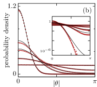
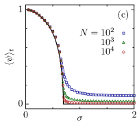
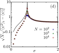
Figure 3: Mean-field binary Vicsek model. (a) The alignment function $\int_{\zeta}\!{{\mathbf{p}}\cdot\delta{\mathbf{p}}}$, for different values of the control parameter $\sigma$. (b) Angular distributions measured at $N=10^{4}$ (symbols) and the corresponding ansatz distributions (lines). From top to bottom: $\sigma=0.25,0.5,0.6,0.675,1$ (respectively, $\psi\simeq 0.94,0.77,0.61,0.32,0.01$). Inset: the same but with vertical log-scale. (c), (d) Average in the steady state of the order parameter and its rescaled standard deviation. Symbols are numerical solution of the Boltzmann equation. Full black lines are theoretical predictions using the von Mises distribution as an ansatz for the angular distribution.

The model is termed as a mean-field one, as a particle can interact with any other one, with no correlation of any kind. By construction, the molecular chaos hypothesis holds exactly for this model, as the master equation that describes the dynamics is exactly the Boltzmann equation. Thus, the discrepancy between the theoretical predictions and the numerical data comes only from finite-size effects, which are negligable here as we will see, and from the inaccuracy of the ansatz. This kind of mean-field models thus provides a way to test for the accuracy of the ansatz in a controlled way. Also, we will compare the results for the present model to a similar one, sharing the same collision rule, but where binary interactions depend on a metric distance. As we will see, the physics of the transition is qualitatively the same for both models.

Let us first look at the theoretical predictions. It is easy to see that ${{\mathbf{p}}\cdot\delta{\mathbf{p}}}=|{\mathbf{p}}|(\cos\eta_{1}+\cos\eta_{2}-|{\mathbf{p}}|)$, where $|{\mathbf{p}}|=2\cos{\textstyle\frac{\Delta}{2}}$. The integration over the collision noises is performed using $\int\mathrm{d}\zeta\equiv\int\mathrm{d}\eta_{1}\mathrm{d}\eta_{2}P(\eta_{1})P(\eta_{2})$. We obtain the alignment function

$$\int\mathrm{d}\zeta\,{{\mathbf{p}}\cdot\delta{\mathbf{p}}}=2\cos{\textstyle\frac{\Delta}{2}}\,\Bigl{(}2e^{-\sigma^{2}/2}-2\cos{\textstyle\frac{\Delta}{2}}\Bigr{)}.$$ (20)

This function of the incoming angular separation $\Delta$, represented in figure 3(a), summarizes the microscopic dynamics averaged over the “internal” degrees of freedom of the scattering (here the collision noise): for $\sigma=0$ it is always positive, all collisions align on average; for $\sigma=\infty$ it is always negative, there is no alignment on average. At intermediate $\sigma$, collision with a large, respectively small, incoming angle separation $\Delta$ align, respectively dis-align. Computing the coefficient $\mu$ now simply consists of averaging this function against the kinetic kernel $K$. Here, there is no spatial dependence of any kind, and $K$ is just a constant. Using equations (13) and (16), we integrate equation (20) over $\int\mathrm{d}\Delta$, obtaining $\mu={\textstyle\frac{8}{\pi}}e^{-\sigma^{2}/2}-2$ and $\xi={\textstyle\frac{4}{3\pi}}e^{-\sigma^{2}/2}$. Solving for $\mu=0$, the transition occurs at $\sigma_{c}=\sqrt{2\log(4/\pi)}\simeq 0.695$ and, because $\xi(\sigma_{c})>0$, the transition is continuous. To extend the predictions to the polar phase, we set $\mathrm{d}\psi/\mathrm{d}t=0$ in equation (8) and solved it numerically, to obtain the order parameter. These predictions are presented in figure 3 in full black lines.

We compare them to numerical results obtained using the following Monte Carlo method [47]. Starting from $N$ random angles $\theta_{i}(t)$, a pair of distinct particles $(i,j)$ is chosen randomly, uniformly. The collision rule is then applied, obtaining the new angles $\theta_{i}(t+1)$ and $\theta_{j}(t+1)$. All other particles keep their angle. The procedure is repeated until the stationary state is reached. We then start to measure averages over time of quantities of interest. In our simulations, these averages typically involved $10^{6}$ collisions, which gives us good enough statistics. Finite-size effects in the simulations are under control, as shown by the scaling in $N$ in figure 3(d). Quite remarkably, the measured angles distributions compare well with the ansatz in the whole range of $\psi$, see figure 3(b). Time averages of the order parameter in the stationary state also compare very well with the theoretical prediction in the whole range of $\psi$, see figure 3(c). Concerning the fluctuations of the order parameter, one must distinguish the isotropic phase from the polar one. In the isotropic phase the predictions are excellent, see figure 3(d), confirming that the correlations are negligible. In the polar phase, the von Mises distribution ansatz is not supposed to be exact, which translates into a qualitative agreement only. Finally, increasing the size of the system, the divergence of the fluctuations at the transition is better and better captured.

3.2 Continuous-time hard disks Vicsek model

We next consider a metric model, with $N$ hard disks of diameter $d_{0}=1$ moving in a periodic box of linear size $L$. The number density is $\rho=N/L^{2}$. In this model, speeds are fixed to $v_{0}=1$. As we do not consider self-diffusion, particles go in a straight line until a collision occurs. Two particles interact when $|{\mathbf{r}}_{1}-{\mathbf{r}}_{2}|=d_{0}$, their velocities are changed following the binary Vicsek collision rule, as already defined in the previous model (alignment to the half-angle and a collision noise with variance $\sigma^{2}$). A way to ensure that the interaction is always binary is to prevent particles from overlapping. This is achieved by noticing that there is only one way to assign the two outcoming velocities to the two particles, out of the two possibilities. We choose to assign the velocities such that particle do not overlap, hence the terming of hard disks. Using this rule, the interaction between particles is binary and the interaction is made instantaneous, which has allowed us to define a continuous-time model. The current model, in the dilute regime where molecular chaos hypothesis holds, is an actual implementation of the one studied theoretically in [12, 13], but not simulated therein. By comparison, in the original Vicsek model, the dynamics are discrete in time. As a consequence, particles behave like disks that can overlap at any time with one or many other particles. Note also that, in the Vicsek dynamics, a scattering event, even if binary, can last many time steps.

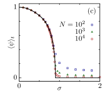
Figure 4: Continuous-time hard disks Vicsek model at density $\rho=10^{-3}$. (a): The alignment function $\int_{\zeta}\!{{\mathbf{p}}\cdot\delta{\mathbf{p}}}$, for different values of the control parameter $\sigma$. (b): Angular distributions measured at $N=10^{4}$ (symbols) and the corresponding ansatz distributions (lines). From top to bottom: $\sigma=0.4,0.6,0.8,0.88,1$ (respectively $\psi\simeq 0.93,0.83,0.59,0.30,0.02$). Inset: the same but with vertical log-scale. (c), (d): Average in the steady state of the order parameter and its rescaled standard deviation. Symbols are numerical data from molecular dynamics simulations. Full black lines are theoretical predictions.

Here again, the collision noise $\sigma$ is used as a control parameter. The collision rule being the same as for the mean-field Vicsek model, the alignment function $\int_{\zeta}\!{{\mathbf{p}}\cdot\delta{\mathbf{p}}}$ is the same as equation (20). For the theoretical description, the only difference stems from the kinetic kernel, which reads here $K(\Delta)\propto\left|\sin(\Delta/2)\right|$, as given by the construction of the Boltzmann cylinder. We also remind the reader that the scattering rate is set by the density, $\lambda\propto\rho$. Again one can compute $\mu$, following equation (13), obtaining $\mu=\frac{8}{\pi}e^{-\sigma^{2}/2}-\frac{16}{3\pi}$, which cancels at $\sigma_{c}=\sqrt{2\log(3/2)}\simeq 0.9005$. We recover the same results as in [12, 13]. We also find that the transition is continuous, $\xi(\sigma_{c})>0$. Remember that this statement only concerns the transition between homogeneous states. It does not rule out the discontinuous transition scenario reported for this system, which involves the destabilization of the homogeneous polar phase with respect to inhomogeneous solutions [12, 13]. Finally, we can also solve numerically equation (8) for the order parameter in the polar phase, see the black lines in figures 4 and 5(a).

We obtained numerical data in the stationary state of molecular dynamics simulations. In the absence of noise, we used an event-driven method, which allowed us to probe more easily the low density regime. Some minimal care has to be taken, as the spatial homogeneity of the stationary states can be destroyed by hydrodynamic instabilities. Practically, these instabilities are known to occur at quite large wavelengths [6, 14], so that we used small-sized systems. We checked explicitly that the simulations run in the homogeneous regime. In particular, no travelling bands were observed in our simulations, even for the largest system $N=10^{4}$. Here also, the theoretical predictions are in very good agreement with the simulation data at low density $\rho=10^{-3}$, see figure 4.

The current model is similar to the mean-field binary Vicsek model defined in the previous section: the binary interaction obeys the same collision rule. Only the scattering rates’ dependance on $\Delta$ differs. Comparing figures 3 and 4, both models share the same qualitative behaviours. In particular, the transition is continuous in both cases. One sees that at the level of homogeneous phases, the nature of the transition is clearly governed by the collision rule rather than by the metric/nonmetric aspect of the interaction.

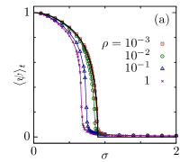
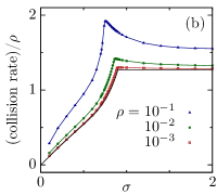
Figure 5: Continuous-time hard disks Vicsek model at densities $\rho=10^{-3}$, $10^{-2}$, $10^{-1}$ and $1$. (a) Polar order parameter. (b) Collision rate, rescaled. For clarity, the data at $\rho=1$ is not plotted. At this density, the rescaled collision rate behaves qualitatively the same as for lower densities, but with much higher values (reaching around $28$ for the maximal value at the transition). Symbols are numerical data, $N=10^{4}$. Black lines are theoretical predictions at vanishing density.

We also investigated finite density effects on the order parameter and the collision rate, as shown in figure 5. Although they are hardly seen at density below $\rho=10^{-3}$, deviations become more and more noticeable as density increases. For the order parameter (figure 5(a)), an increase in density stabilizes the isotropic phase. This is in contrast with the most commonly reported effect of stabilization of the polar phase by density, in the presence of self-diffusion. In the present case, there is no self-diffusion ($D=0$) and the transition shift comes from truly nontrivial correlations. For the collision rate, a quantity most easily measured in event-driven simulations, see figure 5(b), a prediction can be obtained by computing $\lambda\Phi_{f}^{\mathrm{scat}}[1]$, using the von Mises distribution ansatz. The idea is simply to count $+1$ at each collision, instead of $\delta{\mathbf{p}}$ in kinetic equations such as equation (2). The result is plotted as a black full line in figure 5(b). In the isotropic phase, the collision rate is simply the constant $\lambda=4\rho/\pi$. In the polar phase, it decreases smoothly as $\psi$ is increased. This is again a pure kinetic effect. When polar order is higher, particles are more parallel, with smaller relative velocities, so it takes more time before a collision is likely to occur. The collision rate vanishes for $\psi=1$, when all particles are strictly parallel. From the numerical data, we observe first that the overall collision rate is increased as density gets higher; second, that for a given density the collision rate increases as the transition is approached from either side, reaching a finite maximal value at the transition. While the first feature is expected, as it also happens in equilibrium systems [20], the second one indicates a nontrivial dependance of the collision rate with density in the transitional regime. These effects cannot be understood on the basis of the Boltzmann formalism.

3.3 Inelastic self-propelled hard disks

Several works [30, 48, 49] have shown that pairwise dissipative interactions lead to global polarization in swarms of SPPs. In the present model, particles are hard disks of diameter $d_{0}=1$ that collide inelastically. The restitution coefficient $0\leq e\leq 1$ of the inelastic collisions is used as a control parameter for the transition. Between collisions, the dynamics of particle $i$ is given by

$$\frac{\mathrm{d}{\mathbf{r}}_{i}}{\mathrm{d}t} ={\mathbf{v}}_{i},$$ (21)

$$\tau \frac{\mathrm{d}{\mathbf{v}}_{i}}{\mathrm{d}t} =\mathrm{sign}(v_{0}-|{\mathbf{v}}_{i}|)\hat{\mathbf{v}}_{i},$$ (22)

where $\mathrm{sign}(x)$ is $-1$, $0$ or $1$, respectively, when $x$ is negative, zero or positive. The rhs term of equation (22) allows us to use event-driven methods to perform molecular dynamics simulations. It mimics the more standard exponential relaxation of the velocity ${\mathbf{v}}_{i}$ to $\hat{\mathbf{v}}_{i}={\mathbf{v}}_{i}/|{\mathbf{v}}_{i}|$ on a timescale $\tau$. We also studied the case of an exponential relaxation, though in less details, for which we observe that all the results presented below are qualitatively the same. We choose $v_{0}=1$ and $\tau=1$.

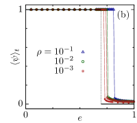
Figure 6: Self-propelled hard disks model with inelastic collisions, $\tau=1$. (a) The alignment function $\int_{\zeta}\!{{\mathbf{p}}\cdot\delta{\mathbf{p}}}$, for different values of the control parameter $e$. (b) Polar order parameter. Symbols: numerical data, $N=1000$ (open symbols), $N=4000$ (full symbols). Black lines are theoretical predictions at vanishing density.

For this model, the $\int_{\zeta}\!{{\mathbf{p}}\cdot\delta{\mathbf{p}}}$ functions are computed numerically by simulating many binary scattering events at some fixed incoming angular separation $\Delta$, varying the impact parameter $b$ uniformly, see figure 6(a). Here, as already stated in the theoretical framework section, the distinction between binary scatterings events and binary collisions is particularly important. A binary scattering event starts at the time of a first collision, when both particles have speed $v_{0}$, with a momentum ${\mathbf{p}}$. After some time, the particles separate forever and the dynamics restore the speed of both particles to $v_{0}$. Only when all these conditions are eventually met does the binary scattering event end and we record the momentum ${\mathbf{p}}^{\prime}$. We insist that while the momentum is conserved by inelastic collisions, it is not by the scattering event; the reason being that after the collision, velocities are being relaxed to $v_{0}$ and momentum is changing, so that in general ${\mathbf{p}}^{\prime}\neq{\mathbf{p}}$. Note also that a single binary scattering event can comprise several inelastic collisions, depending on the parameters of the scattering. From these data, we can compute ${{\mathbf{p}}\cdot\delta{\mathbf{p}}}(b,\Delta)$, then $\mu$ and $\xi$, using equations (13) and (16). We find a transition at $e_{c}\simeq 0.70$. Because $\xi(e_{c})<0$, the transition is predicted to be discontinuous. The results are in full agreement with direct molecular dynamics simulations with a random isotropic state as initial conditions. As shown in figure 6(b), the transition is indeed highly discontinuous.

Around the transition $e=e_{c}$, as seen in figure 6(a), tangential collisions (low $|\Delta|$) align, while frontal collisions (high $|\Delta|$) disalign. This is in total contrast with the binary Vicsek collision rule, see figures 3(a) and 4(a). Note that tangential collisions align for all values of $e$. As a consequence, the fully polar state $\psi=1$ is stable for all values of $e$. Indeed, when $\psi\simeq 1$, particles are all quite parallel, so that binary scattering only occurs at low $|\Delta|$. In this scattering regime, ${{\mathbf{p}}\cdot\delta{\mathbf{p}}}>0$, so that polar order increases back to $\psi=1$. There is thus a coexistence of stability between the $\psi=1$ and $\psi=0$ states, hence a discontinuous transition. Note that one could define a mean-field like version of this model, by considering the model in section 3.1, but with a collision rule given by inelastic collisions, figure 6(a), instead of the Vicsek collision rule, figure 3(a). The results would be qualitatively the same, with a sharp discontinuous transition. Here again, the quantity ${{\mathbf{p}}\cdot\delta{\mathbf{p}}}$ is more important with respect to the nature of the transition than the kinetic kernel. As a final remark, here, as opposed to the previous model, higher densities tend to stabilize the polar phase, even in the absence of self-diffusion.

4 Conclusion

In summary, proposing an ansatz for the velocity angular distribution, we have derived an equation for the evolution of the momentum of systems of polar active particles with fixed speed. The weakly nonlinear analysis around the isotropic state is given by equation (12) and provides an intuitive way of anticipating the transition to collective motion in systems of polar active particles: the existence and the nature of the transition are essentially governed by the way $\int_{\zeta}\!{{\mathbf{p}}\cdot\delta{\mathbf{p}}}$ depends on the incoming angle. As an important consequence, the forward component of momentum change, ${{\mathbf{p}}\cdot\delta{\mathbf{p}}}$, is the proper quantity to characterize the alignment of binary scattering. Also, we tested the fully nonlinear equation on three different kinds of models, and showed that the von Mises ansatz describes quite well the velocity angular distribution, even for large polarization. This shows that knowing the value of the order parameter, alone, already gives much qualitative information about the kinetics. Of course, predictions of more subtle effects in the polar phase should require better approximation schemes. These encouraging results naturally call for the extension of our analysis to models in which the particle speeds are free to fluctuate. Our work may also be adapted to describe the transition towards nematic states or three dimensional systems.

Appendix A On the sign of the cubic term

As the derivation of equation (16) involves the use of an ansatz, it is not “exact” and one should worry about the sign of $\xi$ being wrong. Let us now compare the expression of equation (16) with the one obtained in [17], where the starting point is also the Boltzmann equation, but where the hydrodynamics equations are derived using a different closure scheme. We first briefly describe how these equations are obtained. Starting from the Fourier series $f(\theta,t)=\frac{1}{2\pi}\sum_{k}f_{k}(t)e^{-ik\theta}$, the Boltzmann equation can be written in Fourier space. The result is an infinite number of coupled equations: the time evolution of the $k$th mode is given as a function of the other modes. Next, the following scaling hypothesis is assumed close to the transition [17]: $|f_{k}|\sim\epsilon^{|k|}$ and $\partial_{t}\sim\epsilon$, for some small parameter $\epsilon$. Neglecting all contributions of order $\epsilon^{4}$ and those of higher order, the Boltzmann equation reduces to [17]:

$$\partial_{t}f_{0} =0,$$ (23)

$$\partial_{t}f_{1} =\mu_{1}f_{1}-\xi_{1}f_{1}^{*}f_{2},$$ (24)

$$\partial_{t}f_{2} =\mu_{2}f_{2}+\gamma f_{1}^{2},$$ (25)

The first equation states that a homogeneous density field stays homogeneous. The second one is the analog of our evolution equation for the vectorial order parameter ${\mathbf{P}}$. The third equation describes the evolution of the nematic order parameter. We have discarded the equation for $\partial_{t}f_{3}$ because $f_{1}$ and $f_{2}$ do not depend on $f_{3}$. As long as the scaling hypothesis holds uniformly, these equations can be considered as “exact”. Note that they apply only in the case $\xi_{1}>0$, since $\xi_{1}<0$ would require the inclusion of higher order terms.

In what follows, we suppose that the isotropic state is linearly stable with respect to the nematic phase, hence $\mu_{2}<0$, and consider the slightly polar state, $\mu_{1}>0$ with $\mu_{1}\simeq 0$. As $|f_{1}|\neq 0$, we are free to choose the reference direction by setting $f_{1}^{*}=f_{1}>0$. In the stationnary state, equations (24) and (25) are equated to zero, so as to obtain

$$|f_{1}|^{2}=\frac{\mu_{1}}{\xi_{1}}\frac{|\mu_{2}|}{\gamma},\qquad\qquad f_{2}=\frac{\gamma}{|\mu_{2}|}f_{1}^{2}.$$ (26)

We see from the first equation that one must have $\gamma>0$ and from the second that $f_{2}>0$. The expression of the stationary $f_{2}$ in equation (26) can be used in equation (24), which then reads

$$\partial_{t}f_{1}=\mu_{1}f_{1}-\xi_{1}\frac{\gamma}{|\mu_{2}|}f_{1}^{*}f_{1}^{2}.$$ (27)

We see that the “exact” cubic coefficient is given by $\xi_{1}\gamma/|\mu_{2}|>0$. Note that it has the same sign as $\xi_{1}>0$.

We now come back to our results, obtained from the von Mises distribution ansatz. The expansion in powers of $f_{1}$ of the ansatz in equation (7) reads

$$f_{\psi}(\theta)={\textstyle\frac{1}{2\pi}}+{\textstyle\frac{1}{\pi}}({\psi}\cos\theta+{\psi^{2}}\cos{2\theta}+\dots).$$ (28)

One important difference here is that the second Fourier mode is enslaved to the first one, such that $f_{2}=f_{1}^{2}$, instead of having equation (26). Thus, one finds $\partial_{t}f_{1}=\mu_{1}f_{1}-\xi_{1}f_{1}^{3}$, instead of equation (27). By identifying this equation with equation (15), it is shown that (i) $\mu_{1}=\mu$, as given by equation (13), (ii) $\xi_{1}=\xi$, as given by equation (16), (iii) the cubic term in equation (15) has the correct sign. Thus, if the transition predicted by equation (27) is continuous, equation (15) also predicts a continuous transition: both approaches are consistent. Interestingly, this mainly comes from $f_{2}$ and $f_{1}$ sharing the same sign for a continuous transition, which means that both the polar mode and the nematic modes are in phase, a property also possessed by the von Mises distribution.

When $\xi_{1}<0$, one has to consider higher order “exact” equations. Unfortunately, even the order 7 equations are not well behaved [17].

Appendix B Fluctuations of the order parameter

Here, we derive an expression for the variance of the order parameter. We start from equation (17), the balance equation for the momentum:

$$N({\mathbf{P}}^{\prime 2}-{\mathbf{P}}^{2})=2{\mathbf{P}}\cdot\delta{\mathbf{p}}+\frac{1}{N}{\delta{\mathbf{p}}\cdot\delta{\mathbf{p}}}.$$ (29)

Assuming that the system is nonchiral, we can follow the procedure already used for deriving equation (2). We find

$$\frac{1}{\lambda}\frac{\mathrm{d}{\mathbf{P}}^{2}}{\mathrm{d}t}={2\psi}\,\Phi_{f}^{\mathrm{scat}}\Big{[}\hat{\mathbf{p}}\cdot\delta{\mathbf{p}}\cos\bar{\theta}\Big{]}+\frac{2}{N}\Phi_{f}^{\mathrm{scat}}\Big{[}{\delta{\mathbf{p}}\cdot\delta{\mathbf{p}}}\Big{]}-2\frac{D}{\lambda}\Big{(}\psi^{2}-\frac{1}{N}\Big{)},$$ (30)

with $\Phi_{f}^{\mathrm{scat}}$ defined in Eq. (3). Note that this equality stands at the level of ensemble average. Using the von Mises distribution ansatz, the integration over $\bar{\theta}$ can be performed explicitly and this expression becomes

$$\frac{1}{\lambda}\frac{\mathrm{d}{\mathbf{P}}^{2}}{\mathrm{d}t}={2\psi}F(\psi)+\frac{2}{N}G(\psi)-2\frac{D}{\lambda}\Big{(}\psi^{2}-\frac{1}{N}\Big{)},$$ (31)

where $F(\psi)$ is already given by Eq. (9) and where

$$G(\psi)=\int_{-\pi}^{\pi}\!\frac{\mathrm{d}\Delta}{2\pi}\int\!\mathrm{d}\zeta\,K(\Delta,\zeta)\,\frac{I_{0}\Big{(}2\kappa(\psi)\cos{\textstyle\frac{\Delta}{2}}\Big{)}}{I_{0}^{2}(\kappa(\psi))}\,{\textstyle\frac{1}{2}}{\delta{\mathbf{p}}\cdot\delta{\mathbf{p}}}(\Delta,\zeta).$$ (32)

Now, consider the ensemble averaged stationary state ${\mathbf{P}}_{*}$, and the trajectory of the system around this average: ${\mathbf{P}}(t)={\mathbf{P}}_{*}+\delta{\mathbf{P}}(t)$, with $\delta{\mathbf{P}}(t)$ assumed to be of order $1/\sqrt{N}$. The order 0 of equation (31) gives the condition for the stationary state, $F(\psi_{*})-(D/\lambda)\psi_{*}=0$, while orders $1/\sqrt{N}$ and $1/N$ are respectively

$$\frac{1}{\lambda}\frac{\mathrm{d}{\mathbf{P}}_{*}\cdot\delta{\mathbf{P}}}{\mathrm{d}t} =\left(F^{\prime}(\psi_{*})-\frac{D}{\lambda}\right){\mathbf{P}}_{*}\cdot\delta{\mathbf{P}},$$ (33)

$$\frac{1}{2\lambda}\frac{\mathrm{d}(\delta{\mathbf{P}})^{2}}{\mathrm{d}t} =\left(F^{\prime}(\psi_{*})-\frac{D}{\lambda}\right)(\delta{\mathbf{P}})^{2}+\frac{1}{N}\left(G(\psi_{*})+\frac{D}{\lambda}\right),$$ (34)

where $F^{\prime}(\psi)\equiv{\mathrm{d}F}/{\mathrm{d}\psi}$. The first equation is the stability condition of the stationary state, thus requiring that $F^{\prime}(\psi_{*})<\frac{D}{\lambda}$. Equating the second equation to zero, we get the variance of the order parameter in the stationary state:

$$\textrm{Var}[{\mathbf{P}}]=(\delta{\mathbf{P}})^{2}=-\frac{1}{N}\frac{G(\psi)+D/\lambda}{F^{\prime}(\psi_{*})-D/\lambda}.$$ (35)

The minus sign comes from the denominator being negative. Note that this expression is not expected to be quantitatively accurate in the polar phase. In the isotropic state, this expression becomes equation (18).

References

References

- [1] Ramaswamy S 2010 Annu Rev Conden Ma P 1 323–345
- [2] Marchetti M C, Joanny J F, Ramaswamy S, Liverpool T B, Prost J, Rao M and Simha R A 2013 Rev. Mod. Phys. 85 1143–1189
- [3] Vicsek T, Czirók A, Ben-Jacob E, Cohen I and Shochet O 1995 Phys. Rev. Lett. 75 1226–1229
- [4] Czirók A, Stanley H E and Vicsek T 1997 Journal of Physics A: Mathematical and General 30 1375
- [5] Grégoire G and Chaté H 2004 Phys. Rev. Lett. 92 –
- [6] Chaté H, Ginelli F, Grégoire G and Raynaud F 2008 Phys. Rev. E 77 –
- [7] Ginelli F and Chaté H 2010 Phys. Rev. Lett. 105 168103
- [8] Vicsek T and Zafeiris A 2012 Physics Reports 517 71–140
- [9] Toner J, Tu Y and Ramaswamy S 2005 Annals of Physics 318 170–244
- [10] Toner J and Tu Y 1995 Phys. Rev. Lett. 75 4326–4329
- [11] Toner J and Tu Y 1998 Phys. Rev. E 58 4828–4858
- [12] Bertin E, Droz M and Grégoire G 2006 Phys. Rev. E 74 22101
- [13] Bertin E, Droz M and Grégoire G 2009 Journal of Physics A Mathematical General 42 445001
- [14] Ihle T 2011 Phys. Rev. E 83 030901
- [15] Chou Y L, Wolfe R and Ihle T 2012 Phys. Rev. E 86 021120
- [16] Peshkov A, Ngo S, Bertin E, Chaté H and Ginelli F 2012 Phys. Rev. Lett. 109 098101
- [17] Peshkov A, Bertin E, Ginelli F and Chaté H 2014 The European Physical Journal Special Topics 223 1315–1344 ISSN 1951-6355 URL http://dx.doi.org/10.1140/epjst/e2014-02193-y
- [18] Ihle T 2014 Eur. Phys. J. Special Topics 223 1293–1314
- [19] Caussin J B, Solon A, Peshkov A, Chaté H, Dauxois T, Tailleur J, Vitelli V and Bartolo D 2014 Phys. Rev. Lett. 112 148102
- [20] Hansen J P and McDonald I R 1976 Theory of simple liquids (London: Academic Press)
- [21] Kudrolli A, Lumay G, Volfson D and Tsimring L S 2008 Phys. Rev. Lett. 100
- [22] Deseigne J, Dauchot O and Chaté H 2010 Phys. Rev. Lett. 105
- [23] Palacci J, Cottin-Bizonne C, Ybert C and Bocquet L 2010 Phys. Rev. Lett. 105 –
- [24] Theurkauff I, Cottin-Bizonne C, Palacci J, Ybert C and Bocquet L 2012 Phys. Rev. Lett. 108 268303
- [25] Deseigne J, Léonard S, Dauchot O and Chaté H 2012 Soft Matter 8 5629–5639
- [26] Bricard A, Caussin J B, Desreumaux N, Dauchot O and Bartolo D 2013 Nature 503 95–98
- [27] Palacci J, Sacanna S, Steinberg A P, Pine D J and Chaikin P 2013 Science 339 936–940
- [28] Kumar N, Soni H, Ramaswamy S and Sood A K 2014 Nat. Comm. 5 4688
- [29] Peruani F, Deutsch A and Bär M 2006 Phys. Rev. E 74 30904
- [30] Grossman D, Aranson I S and Ben-Jacob E 2008 New Journal of Physics 10 023036
- [31] Henkes S, Fily Y and Marchetti M C 2011 Phys. Rev. E 84 –
- [32] Fily Y and Marchetti M C 2012 Phys. Rev. Lett. 108(23) 235702
- [33] Redner G S, Hagan M F and Baskaran A 2013 Phys. Rev. Lett. 110 055701
- [34] Weber C A, Hanke T, Deseigne J, Léonard S, Dauchot O, Frey E and Chaté H 2013 Phys. Rev. Lett. 110 208001
- [35] Solon A P and Tailleur J 2013 Phys. Rev. Lett. 111(7) 078101
- [36] Solon A P, Chaté H and Tailleur J 2015 Phys. Rev. Lett. 114(6) 068101
- [37] Romensky M, Lobaskin V and Ihle T 2014 Phys. Rev. E 90(6) 063315
- [38] Ballerini M, Cabibbo N, Candelier R, Cavagna A, Cisbani E, Giardina I, Lecomte V, Orlandi A, Parisi G, Procaccini A, Viale M and Zdravkovic V 2008 Proceedings of the National Academy of Sciences 105 1232–1237
- [39] Degond P, Appert-Rolland C, Pettré J and Theraulaz G 2013 Kinetic and Related Models 6(4) 809–839
- [40] Albi G, Balagué D, Carrillo J A and von Brecht J 2014 SIAM J. Appl. Math. 74 794–818
- [41] Hanke T, Weber C A and Frey E 2013 Phys. Rev. E 88(5) 052309
- [42] Aldana M, Dossetti V, Huepe C, Kenkre V and Larralde H 2007 Phys. Rev. Lett. 98 95702
- [43] Kardar M 2007 Statistical Physics of Particles (Cambridge)
- [44] Watson G 1982 Journal of Applied Probability 19 265–280
- [45] Degond P, Frouvelle A and Liu J G 2013 J. Nonlinear Sci. 23 427–456
- [46] Chepizhko O and Kulinskii V 2014 Physica A 415 493–502
- [47] Bird G A 1970 Physics of Fluids (1958–1988) 13 2676–2681
- [48] Lobaskin V and Romenskyy M 2013 Phys. Rev. E 87(5) 052135
- [49] Coburn L, Cerone L, Torney C, Couzin I D and Neufeld Z 2013 Physical Biology 10 046002