Beamline Instrumentation for Future Parity-Violation Experiments

Abstract

The parity-violating electron scattering community has made tremendous progress over the last twenty five years in their ability to measure tiny asymmetries of order 100 parts per billion (ppb) with beam-related corrections and systematic errors of a few ppb. Future experiments are planned for about an order of magnitude smaller asymmetries and with higher rates in the detectors. These new experiments pose new challenges for the beam instrumentation and for the strategy for setting up the beam. In this contribution to PAVI14 I discuss several of these challenges and demands, with a focus on developments at Jefferson Lab.

1 Introduction

Parity-violation experiments exploit the fact that a component of the weak interaction changes sign under a parity transformation, which isolates the effects due to the weak interaction and provides a tool to study a variety of physics topics. In electron scattering experiments, the parity is transformed by reversing the longitudinal spin, or helicity, of the incident electrons. This method relies crucially on a clean helicity reversal, such that no other beam parameter, e.g. the angle or the energy, is affected. Such effects would cause a systematic error since the much larger electromagnetic interaction is very sensitive to these parameters.

2 Setting up the Electron Beam

In an ideal electron-scattering parity-violation experiment, the two beams corresponding to the two helicity states would be identical. In practice, however, imperfections in the laser optics system at the polarized source will produce some level of coupling of the helicity to other beam properties. The enormous efforts to suppress this coupling at the laser source is described in several references (e.g. [1, 2]) and will not be discussed here. The experience at Jefferson Lab is that after these efforts one is left with residual helicity-correlated beam position differences of typically 50 nm in the beam at the injector which need further suppression.

2.1 Adiabatic Damping

Linear beam optics in a perfectly tuned accelerator can lead to a reduction in position differences from the injector to the experimental hall due to the adiabatic damping of phase space area for a beam undergoing acceleration [3]. The projected beam size and divergence, and thus the difference orbit amplitude (defined as the size of the excursion from the orbit of the design tune), are proportional to the square root of the emittance multiplied by the beta function at the point of interest. Ideally, the position differences become reduced by a factor of $\sqrt{\frac{P}{P_{I}}}$ where $P$ is the momentum after acceleration and $P_{I}$ is the momentum at the injector. For example, at JLab with $P_{I}=335$ keV and $P=6$ GeV, the damping factor would be $\sim 100$. This also implies that the region near the injector is a sensitive location to measure and apply feedback on these position differences, if signals from the beams of the different experimental halls could be measured separately.

Deviations from this ideal reduction factor can however occur mainly due to two effects. The presence of XY coupling can potentially lead to growth in the emittance in both X and Y planes, while a beam line that does not match well with design, due to imperfections, often results in growth in the beta function. Both effects can translate into growth in the difference orbit amplitude and a reduction in the adiabatic damping achieved. Matching the sections of the accelerator is an empirical procedure in which the Courant-Snyder parameters  [4] are measured by making kicks in the beam orbit, and the quadrupoles are adjusted to fine-tune the optics  [5]. For future experiments, an investment should be made by accelerator experts to better understand and automate this procedure so that it can be performed efficiently.

2.2 Spin Flips and Feedback

In order to maintain low systematic errors there must be at least one, and preferably several, methods to reverse the helicity. The helicity reversals should be uncoupled to other parameters which affect the cross section. The rapid, random helicity reversal done at the polarized source does a good job of reducing the correlation with noise; however, the act of changing the sign of a 3 kV voltage on the Pockel Cell (PC) to flip the helicity of the laser inevitably leaves a small residual systematic in the beam.

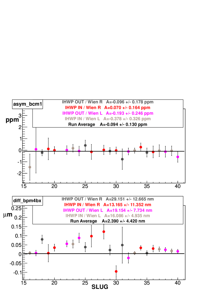
Figure 1: PREX-I [6] helicity-correlated charge asymmetries (top) and position differences (bottom) on a representative monitor versus slug (a slug is $\sim 1$ day of running). The different colors correspond to four different combinations of insertable halfwave plate (IHWP) and Wien used for slow sign reversal. To illustrate the systematics, the data points are plotted without sign correction for the helicity flip. The final average with all sign corrections is shown by the black horizontal bar and was controlled at the 5 nm level averaged over the PREX-I run.

A standard slow-reversal method is a half-wave ($\lambda$/2) plate, which is periodically inserted into the injector laser optical path, reversing the sign of the electron beam polarization relative to both the electronic helicity control signals and the voltage applied to the polarized source laser electro-optics. Roughly equal statistics are collected with this waveplate inserted and retracted, suppressing many possible sources of systematic error. In addition to using the ($\lambda$/2) plate, the E158 experiment [7] ran at two beam energies to make use of the g-2 precession of spin to achieve another slow reversal.

The $4\pi$ Spin Flipper is a relatively new apparatus developed at Jefferson Lab [8]. It is a section of beamline consisting of two Wien filters with a solenoid magnet sandwiched in between. By reversing the spin polarization with the solenoids, rather than with the Wien filters, a clean flip is achieved with minimal change in the beam trajectory or beam envelope. The sign of the B-field in the solenoid determines the beam spin direction, while the optical focusing varies, in first order, as $B^{2}$ and is therefore insensitive to the sign.

The advantage of having multiple slow reversals is demonstrated by the monitor difference from PREX (fig  1). Note, a “BPM” is a beam position monitor, and a “BCM” is a beam current monitor. Without the reversals, the position differences remained at the $\sim$ 50 nm level (the points without sign correction) averaged over the experiment; with the reversals, the differences averaged to the $\sim 5$ nm level (the black lines) and became a negligible correction [6].

For the purpose of measuring the sensitivity of helicity correlations in beam parameters, and for possibly providing feedback to reduce these, the injector group has installed a set of fast, pulsed magnets at the CEBAF injector. A dipole magnet can produce helicity correlated position or angle differences, while using an arrangement of weak quadrupole magnets, the spot-size differences at the interesting level of $10^{-4}$ can be induced as well (see section  5.1). While all parity experiments employ active feedback on the charge asymmetry, future experiments will likely need active feedback on other parameters of the beam, such as E158 did with piezomirrors in the polarized source laser optics  [1].

3 Normalization

When computing the asymmetry from detector signals one must normalize to beam charge in each helicity state. In addition, the measured asymmetry must be normalized by beam polarization $P_{e}$ and by a function of the four-momentum transfer $Q^{2}$. Here we will neither discuss the measurements of $Q^{2}$ nor the beam polarimetry. The vital topic of polarimetry was covered at this conference in contributions by David Gaskell, Timothy Gay, and Partricia Bartolome.

For the beam charge normalization, the “noise floor”, or intrinsic electronic noise of the charge monitors, is important. This is measured by computing the difference of charge asymmetries measured by two monitors and computing the width $\sigma_{\rm diff}$ in the difference. At Jefferson Lab, at present, this $\sigma_{\rm diff}$ extrapolated to high currents indicates a noise floor of 60 ppm which will need to be improved by a factor of 6 for the MOLLER experiment [23], requiring more research on these monitors and the associated electronics. The noise in the BPM monitors and the intrinsic noise in the beam at 6 GeV both appear to be adequate for planned experiments, but the beam properties after the 11 GeV upgrade have yet to be studied.

New digital-signal-processing electronics are being deployed for the BPM and BCM monitors at Jefferson Lab [9] which have the advantages of reduced noise and higher bit resolution (32 bits). The electronics process in an FPGA the signals from the stripline BPMs or the cavity BPMs and BCMs. Consumers of these data will need to send an electronic gate to define the time of each integration period and will receive via a fiber optic link the digital results, i.e. the integrated charge or position, for data acquisition. The fiber optic link will also have the advantage of helping to break ground loops.

4 First Order Beam Corrections

The scattering rate from a target depends on the five “first order” parameters: energy, position and angle of the beam, i.e. $(E,x,y,{\theta}_{x},{\theta}_{y})$ which are measured by beam monitor signals $M_{i}$. The “first order” systematics involve the possible helicity-correlations in these parameters and the sensitivities (derivatives) of the cross section.

$$A=A_{D}-A_{I}-\sum_{i}{\beta_{i}\hskip 1.4457pt\langle\Delta M_{i}\rangle}$$ (1)

Here $A_{D}$ is the asymmetry in the detector, $A_{I}$ is the asymmetry in the beam current, and the $\Delta M_{j}$ are helicity-correlated differences in a set of beam monitors $M_{i}$ which are linearly related to the beam parameters. The coefficients $\beta_{j}$ are measured during the experiment by deliberately moving the beam small amounts in all its parameters, including energy, to measure the sensitivity to these. Ideally, the corrections to $A_{D}$ are negligible, and the systematic errors, which by definition is the error in these corrections, are also negligible. That has been the case for the earlier parity experiments done at JLab [10, 11] as well as at Mainz [12].

Future parity-violation experiments [23, 13] at Jefferson Lab will require BCMs capable of measuring charge asymmetry widths of 10 ppm at 2 kHz and position differences of 3 $\mu$m. While the Qweak experiment [14, 15] demonstrated accuracies in beam monitors close to these values and established an adequately small jitter in the beam parameters, more research will be necessary to push the accuracy of the monitors to robustly satisfy the requirements, and the beam properties remain to be reestablished after the upgrade to 12 GeV of the CEBAF accelerator.

5 Higher Order Beam Corrections and Backgrounds

The next generation of parity-violation experiments will require a better understanding and control of the “higher order” corrections, a term used to describe both the sensitivity to higher derivatives of the cross section with respect to beam parameters, as well as other parameters that are not characterized by the set of five parameters measured by the BPM or BCM monitors. Two examples of these effects are : 1) “spot size” : in this effect, a normal-sized beam with no tails has helicity-correlated fluctuations in its RMS;  and 2) “beam halo” : defined as significant tails in the beam (many $\sigma$ in radius) which can have a helicity component and which can scrape and cause backgrounds.

5.1 Spot Size Sensitivity

The effects of spot size can estimated analytically for a spectrometer experiment like PREX [16]. Let $w$ be the RMS width of the beam and $\Delta w$ be the helicity correlated difference in $w$, with $\Delta w\ll w$. For a very narrow (pinhole) acceptance at a distance $D$ from the target, the accepted angular range is $\delta\theta=\frac{w}{D}$. While the scattering rate $R$ depends strongly on the angle $\theta$ the first-derivative term involving $dR/d\theta$ is suppressed because as the angle increases the rate decreases. The beam-width effect is therefore second-order, and the helicity-correlated differences in the rate $R$ is

$$\Delta R=\Delta\hskip 1.4457pt\langle\frac{1}{2}\hskip 2.8903pt\frac{d^{2}R}{d\theta^{2}}\hskip 2.8903pt\frac{w^{2}}{D^{2}}\rangle\hskip 2.8903pt=\hskip 2.8903pt\frac{d^{2}R}{d\theta^{2}}\hskip 1.4457pt\frac{w\Delta w}{D^{2}}$$ (2)

For PREX on ²⁰⁸Pb, the false asymmetry can be estimated [16] by using a typical beam width $w=100\mu$m and assuming control of $\Delta w$ to an accuracy of $10$ nm averaged over a few days, obtaining a false asymmetry systematic of 2 ppb. Note that the PREX physics asymmetry is 0.5 ppm and the error goal is 3% which is 15 ppb. This establishes a goal to be able to control and measure the helicity correlated spot size differences $\Delta w$ to an accuracy of about 10 nm averaged over a few days. While this may seem difficult, I note that comparable accuracies have already been achieved for the first order parameters.

5.2 Measuring Spot Size

While there have been very accurate longitudinal spot size measurements at the 80 fs level [17], the measurements of transverse spot size variations, which use for example wire scanners [18] or synchrotron light interferometry [19], have not yet reached a level of accuracy desirable for next-generation parity experiments. Microwave cavity monitors have been proposed [20] as a away to accomplish this. These monitors are built in a size and shape to achieve resonance at a particular eigenfunction of the electric field; this provides the desired sensitivity to the beam current and the position [21]. Assuming a cylindrical cavity, the monitor’s signal is proportional to $IE\sim J_{n}(x)$, where $I$ is beam current, $E$ is the electric field, and $J_{n}(x)$ is the Bessel Function of the first kind, “n” denotes the mode, and $x$ is the distance from beam center. A current monitor uses the beam to excite the “n=0” mode, which is relatively insensitive to beam position. A position monitor uses “n=1”, which to first order has a linear dependence on the beam position. A square cavity yields a similar result with sine functions as the eigenfunctions. The question is: Can spot size be determined using a higher order mode $n>1$ ?

If $w$ is the spot size (section  5.1) and the nominal position in the cavity is $x$, the average of the $n=2$ Bessel Function is to first order

$$\langle J_{2}(x)\rangle\hskip 3.61371pt\propto\hskip 3.61371pt\langle x^{2}\hskip 2.8903pt+\hskip 2.8903ptxw\rangle$$ (3)

The signal from such a cavity will be a mixture of spot size and position, as well as beam current. Combining this signal with the signals from lower-mode cavities to normalize to beam current $I$ and average position $\langle x\rangle$, it might be possible to extract the sensitivity to the spot size $w$ and its helicity dependence. Another possible non-invasive method to measure spot size is to use a stripline position monitor with 8 or 16 poles, which is being tried at some facilities [22].

6 Luminosity and Halo Monitors

A parity experiment in an open geometry like Qweak [14, 15] or MOLLER [23] might suffer from dangerous backgrounds as a result of beam halo. The Qweak experiment used a Beam Halo monitor to measure and correct for helicity correlations in the halo background. This detector consisted of a thin aluminum plate surrounded by lead-shielded lucite detectors and photomultipliers.

Another tool available for monitoring the beam properties as well as target boiling is a Luminosity Monitor (“Lumi”), which consists of detectors placed symmetrically about the beam downstream of the target at small angles. For Qweak [15], four quartz blocks read out by lightguides connected to photomultipliers were used primarily to detector the Møller electrons but also served to check the backgrounds from upstream collimators and beam halo. The Lumi can also serve to establish a noise floor since the rates are much higher than in the main detector and the width of the asymmetry will be narrower.

Future parity experiments will need a judicious choice of monitoring and collimation to reduce and to monitor beam halo and other backgrounds. The experimental apparatus should be simulated carefully and methods to reduce halo in the accelerated beam, and to make it more predictable, should be studied.

7 Acknowledgments

The author gratefully acknowledges discussions with Arne Freyberger, Joe Grames, Goeffrey Krafft, Dave Mack, John Musson, Mark Pitt, Matt Poelker, Brock Roberts, Yves Roblin, and Riad Suleiman. This work was supported by the Jefferson Science Associates, LLC, which operates Jefferson Lab for the U.S. DOE under U.S. DOE contract DE-AC05-060R23177.

References

- [1] T. B. Humensky et al. Nucl. Instr. and Methods A521 (2004) 261.
- [2] K.A. Aniol et al., Phys. Rev. C69 (2004) 065501.
- [3] D.A. Edwards and M.J. Syphers, An Introduction to the Physics of High Energy Accelerators, Wiley Interscience (1993).
- [4] E.D. Courant and H.S. Snyder, Annals of Physics 3 (1958) 1.
- [5] Y. Chao, “Measuring and Matching Transport Optics at Jefferson Lab”, Proc. of the 2003 Particle Accelerator Conference, Oregon, 2003.
- [6] S. Abrahamyan et al., Phys. Rev. Lett. 108, (2012) 112502.
- [7] P.L. Anthony et al. Phys. Rev. Lett. 95 (2005) 08161; Phys. Rev. Lett. 92 (2004) 181602;
- [8] J. Grames et al., ”Two Wien Filter Spin Flipper”, Proceedings of 2011 Particle Accelerator Conference, New York, NY, USA (TUP025).
- [9] H. Dong et al, Conf.Proc. C0505161 (2005) 3841; JLab Tech Note JLAB-TN-14-028.
- [10] K.A. Aniol et al., Phys. Lett. B 509 (2001) 211; K.A. Aniol et al., Phys. Rev. C69 (2004) 065501; K.A. Aniol et al., Phys. Rev. Lett. 96 (2006) 022003; K.A. Aniol et al., Phys. Lett. B635 (2006) 275; A. Acha et al., Phys. Rev. Lett. 98 (2007) 032301; Z. Ahmed et al., Phys. Rev. Lett. 108, 112502 (2012).
- [11] D.H. Beck, Phys. Rev. D 39 (1989) 3248; D.S. Armstrong et al., Phys. Rev. Lett. 95 (2005) 092001; D. Androic et al., Phys. Rev. Lett. 104 (2010) 012001.
- [12] F.E. Maas et al., Phys. Rev. Lett. 93 (2004) 022002; F.E. Maas et al., Phys. Rev. Lett. 94 (2005) 152001; S. Baunack et al., Phys. Rev. Lett. 102 (2009) 151803.
- [13] P. Souder et al. The PVDIS SOLID Experiment Proposal, 2009, unpublished.
- [14] D. Androic et al. Phys. Rev. Lett. 111 141803 (2013) 14.
- [15] T. Allison al, arXiv 1409.7100.
- [16] Paul Souder, “Systematic Errors Due to Beam Widths”, PREX Tech Note, unpublished (2008).
- [17] D.X. Wang, G.A. Krafft, C.K. Sinclair, Phys Rev E 57 (1998) 2283.
- [18] A.P. Freyberger, Proc. of the 2003 Particle Accelerator Conference.
- [19] P. Chevstov et al, Proc of EPAC 2004, Lucerne (2004).
- [20] Dave Mack and Mark Wissman, “A Microwave Cavity Beam Spot Size Monitor for Qweak”, Qweak Tech Note, unpublished (2006).
- [21] R. Scholl et al SLAC-PUB-0277 (1967); David H. Whittum et al, ARDB Technical Note 134 for the E158 Experiment (1997).
- [22] P. Li et al IEEE Nuclear Science Symposium Conference Record (2007) 1675.
- [23] K. Kumar et al. The MOLLER Experiment Proposal, 2011, unpublished.