A Black-Hole Primer:
Particles, Waves,
Critical Phenomena and Superradiant Instabilities
Bad Honnef School “GR99”
Emanuele Berti
(14 October 2014)
Contents
toc
Chapter 1 Introduction
These informal notes were prepared for a lecture on black-hole physics delivered at the DPG Physics School “General Relativity 99”, organized by Gerhard Schäfer and Clifford M. Will and held on Sep 14–19 2014 at the Physikzentrum in Bad Honnef, Germany. The goal of the notes is to introduce some key ideas in black hole physics that highlight an intimate connection between the dynamics of particles and waves in black-hole spacetimes. More specifically, I will show that the geodesic motion of particles is related to the characteristic properties of wave scattering in black hole backgrounds. I will introduce the proper oscillation modes of a black hole (“quasinormal modes”) and illustrate how they are related with the stability of circular orbits for massless particles in the geometrical optics limit. Finally, I will explain the basic ideas behind superradiance, and I will give a concise introduction to “hot topics” in current research. The prerequisite background is a knowledge of physics at the advanced undergraduate level, namely nonrelativistic quantum mechanics and General Relativity at the level of Hartle [45], Schutz [84] or Carroll [22]. In particular, I will assume some familiarity with the Einstein field equations, the Schwarzschild metric and the Kerr metric.
I will focus on the core physics, rather than the mathematics. So – whenever given the choice – I will consider the simplest prototype problem (one that can quickly be solved with pen and paper), providing references to generalizations that involve heavier calculations but no substantial new physics.
In Chapter 2, after a short review of the derivation of the geodesic equations from a variational principle, I will focus on geodesics in spherically symmetric spacetimes (more in particular, the Schwarzschild spacetime). I will discuss orbital stability in terms of Lyapunov exponents, then I will apply the formalism to compute the principal Lyapunov exponent for circular null geodesics in Schwarzschild.
In Chapter 3 I will introduce a simple prototype for black-hole perturbations induced by a “test” field, i.e. a massive scalar field. I will separate variables for the corresponding wave equation (the Klein-Gordon equation), and then I will discuss two techniques to solve the associated eigenvalue problem: Leaver’s continued fraction method and the WKB approximation. Last but not least, I will show how the application of the same techniques to rotating (Kerr) black holes leads to the interesting possibility of superradiant amplification.
In Chapter 4 I will use this “theoretical minimum” to introduce some exciting ideas in black hole physics that have been a focus of recent research, in particular: (1) critical phenomena in black-hole binary encounters, and (2) the idea that astrophysical measurements of black-hole spins can constrain the mass of light bosonic fields (via superradiant instabilities).
For further reading on black holes I recommend Shapiro and Teukolsky’s Black holes, white dwarfs, and neutron stars [86], Frolov and Novikov’s Black hole physics: Basic concepts and new developments [38], Chandrasekhar’s The Mathematical Theory of Black Holes [23] and a recent overview article by Teukolsky [92]. For reviews of black-hole perturbation theory, see [56, 71, 12]. Throughout these notes, unless otherwise stated, I will use geometrical units () and I will follow the sign conventions of Misner, Thorne and Wheeler [66].
1.1 Newtonian Black Holes?
Popular articles on black holes often mention that a Newtonian analog of the black-hole concept (a “dark star”) was first proposed by Michell in 1783. Michell’s idea was simple: the escape velocity of an object at the surface of a star (or planet) with mass is
| (1.1.1) |
If we consider light as a corpuscle traveling at speed , light can not escape to infinity whenever . Therefore the condition for existence of “dark stars” in Newtonian mechanics is
| (1.1.2) |
Remarkably, a similar situation holds in Einstein theory. The field equations tell us that there exist vacuum, spherically symmetric solutions of the field equations describing a source of mass such that the (areal) radius of the horizon – the region from which even light can not escape – corresponds to the equal sign in (1.1.2). They also tell us that the redshift of light emitted from the horizon is infinite: the object is perceived as completely black. A major difference is that in Newtonian gravity particles can cross the surface , while in General Relativity this surface marks a causal boundary in spacetime.
What popular books usually do not address is the following question: can Michell’s solutions exist in nature? In General Relativity, the most compact stars are made out of incompressible matter and they correspond to the Buchdahl limit (see e.g. [84]), but they are not black holes! In Newtonian mechanics, a naive argument tells us that as we pile up more and more material of constant density , the ratio increases:
| (1.1.3) |
This equation would seem to suggest that Michell’s dark stars could indeed form. Unfortunately, we forgot to include the binding energy :
| (1.1.4) |
Once we do, the total mass of the hypothetical dark star is given by the rest mass plus the binding energy:
| (1.1.5) |
where the upper limit is obtained by maximizing the function in the range (1.1.2). Thus, the “dark star criterion” (1.1.2) is never satisfied, even for the unrealistic case of constant-density matter. In fact, the endpoint of Newtonian gravitational collapse depends very sensitively on the equation of state, even in spherical symmetry [39, 64].
Despite the physical impossibility to construct Newtonian black holes with “ordinary” matter, the genesis of the idea is historically interesting. The email from Steve Detweiler to James Fry reported in Box 1.1 (reproduced here with permission from Steve Detweiler - thanks!) has some amusing remarks on Reverend Michell’s contributions to science.
-
Box 1.1 Steve Detweiler’s email to James Fry on Reverend Michell’s “black holes” (and other amusing things)
Date: Tue, 25 Aug 98 08:11:25 -0400
From: Steve Detweiler
To: James Fry
Subject: Re: Newtonian black holesJim,
The Reverend John Michell in a letter to his good friend Henry Cavendish that was published in Transactions of the Royal Society in 1784. Here is an excerpt of a summary I made in a letter to a friend–I think it’s amusing!
The reference is ”On the Means of discovering the Distance, Magnitude, etc. of the Fixed Stars, in consequence of the Diminution of the Velocity of their Light, in case such a Diminution should be found to take place in any of them, and such other Data should be procured from Observations, as would be farther necessary for that Purpose”, by the Rev. John Michell, B.D.F.R.S., in a letter to Henry Cavendish, Esq. F.R.S. and A.S., Philosophical Transactions of the Royal Society of London, Vol. LXXIV, 35-57 (1784). We sure don’t title papers the way they used to.
I was at Yale when I found out about this article, so I called up their rare books library and was informed that 1784 really wasn’t so long ago and that the volume I wanted was on the stacks in the main library. I just checked it out, they had to glue in a new due date sticker in back, and I had it on my desk for six months.
Michell’s idea is to determine the distance to the stars by measuring the speed of light from the stars–the further away the star is, the slower the light would be moving. He conceded that there would need to be improvement in prism quality for this to be possible, but he thought it was within reach. It’s an interesting paper, the arguments are all geometrical, where there should be an equation he writes it out long hand, all the s’s look like f’s, and it’s fun to read. Somewhere in the middle of the paper (paragraph 16), he notes that if a star were of the same density as the sun but with a radius 500 times larger, then the light would be pulled back to star and not escape. He even surmises that we might be able to detect such an object if it were in a binary system and we observed the motion of the companion. So we should have celebrated the Black Hole Bicentennial back in 1984!
And Michell was an interesting fellow. He wrote 4 papers that I know about, and I think these are in chronological order. In one paper (1760), he notes a correspondence between volcanos and fault lines in the earth’s crust and first suggested that earthquakes might be caused by masses of rocks shifting beneath the earth’s surface. In another, Michell (1767) estimates that if the stars were just scattered randomly on the celestial sphere then the probability that the Pleiades would be grouped together in the sky is 1 part in 500,000. So he concluded that the Pleiades must be a stellar system in its own right—this is the first known application of statistics to astronomy. In a third paper, he devised a torsion balance and used it to measure the dependence of the force between magnetic poles. His fourth paper has the black hole reference. After that work, he started a project to modify his magnetic-force torsion balance to measure the force of gravity between two masses in the laboratory. Unfortunately, he died in the middle of the project. But his good friend, Henry Cavendish, stepped in, made important improvements and completed the experiment! In his own paper, Cavendish gives a footnote reference to Michell.
1.2 The Schwarzschild and Kerr Metrics
I refer to the textbooks by Hartle [45], Schutz [84] or Carroll [22] for introductions to the Schwarzschild and Kerr spacetimes that provide the necessary background for these lecture notes. Here I collect the relevant metrics and a few useful results, mainly to establish notation. The Schwarzschild metric reads
| (1.2.6) |
where is the black-hole mass. The Kerr metric for a black-hole with mass and angular momentum reads:
where
| (1.2.8) |
The event horizon is located at the larger root of , namely
| (1.2.9) |
Stationary observers at fixed values of and rotate with constant angular velocity
| (1.2.10) |
For timelike observers, the condition yields
| (1.2.11) |
where I have used (1.2.10) to eliminate . The quantity in square brackets must be negative; but since is positive, this is true only if , where denotes the two roots of the quadratic, i.e.
| (1.2.12) |
Note that when , i.e. , which occurs at
| (1.2.13) |
Observers between and must have , i.e. no static observers exist within . This is the reason why the surface is called the “static limit”. The surface is also called the “boundary of the ergosphere”, because this is the region within which energy can be extracted from the black hole via the Penrose process (a close relative of the superradiant amplification that I will discuss in Chapter 3).
Chapter 2 Particles
2.1 Geodesic Equations from a Variational Principle
In Einstein’s theory, particles do not fall under the action of a force. Their motion corresponds to the trajectory in space-time that extremizes111The “principle of least action” is a misnomer, because the action is not always minimized along a geodesic: it can either have a minimum or a saddle point (see [76] for an introduction and [75] for a detailed discussion in General Relativity, as well as references to the corresponding problem in classical mechanics). the proper interval between two events. Mathematically, this means that the equations of motion (or “geodesic equations”) can be found by a variational principle, i.e. by extremizing the action
| (2.1.1) |
where the factor of in the definition of the Lagrangian density was inserted for later convenience. Therefore our task is to write down the usual Euler-Lagrange equations
| (2.1.2) |
for the Lagrangian
| (2.1.3) |
Here I introduced the notation
| (2.1.4) |
for the particle’s four-momentum, a choice that allows us to consider both massless and massive particles at the same time (cf. [86, 76] for more details). The “affine parameter” can be identified with proper time (more precisely, with ) along the timelike geodesic of a particle of rest mass . The canonical momenta associated with this Lagrangian are
| (2.1.5) |
and they satisfy
| (2.1.6) |
More explicitly, introducing the usual notation , one has
| (2.1.7) | |||
| (2.1.8) | |||
| (2.1.9) |
and therefore
| (2.1.10) |
Now, and are dummy indices. By symmetrizing one gets , and finally
| (2.1.11) |
From the definition of the Christoffel symbols
| (2.1.12) |
it follows that
| (2.1.13) |
i.e. the usual geodesic equation.
2.2 Geodesics in Static, Spherically Symmetric Spacetimes
In most of these notes I will consider a general static, spherically symmetric metric (not necessarily the Schwarzschild metric) of the form
| (2.2.14) |
This metric can describe (for example) a spherical star, and it reduces to the Schwarzschild metric (see e.g. [45, 84, 22]) when . For brevity, in the following I will omit the -dependence of and . For this metric, the Lagrangian for geodesic motion reduces to
| (2.2.15) |
The momenta associated with this Lagrangian are
| (2.2.16) | |||||
| (2.2.17) | |||||
| (2.2.18) | |||||
| (2.2.19) |
The Hamiltonian is related to the Lagrangian by a Legendre transform:
| (2.2.20) |
and it is equal to the Lagrangian, as could be anticipated because the Lagrangian (2.1.3) is “purely kinetic” (there is no potential energy contribution). Therefore and they are both constant.
As a consequence of the static, spherically symmetric nature of the metric, the Lagrangian (2.2.15) does not depend on and . Therefore the - and -components yield two conserved quantities and :
| (2.2.21) | |||
| (2.2.22) |
The radial equation reads
| (2.2.23) |
The remaining equation tells us that
| (2.2.24) |
so if we choose when it follows that , and the orbit will be confined to the equatorial plane at all times. In conclusion:
| (2.2.25) | |||
| (2.2.26) |
where is the particle’s energy and is the orbital angular momentum (in the case of massive particles, these quantities should actually be interpreted as the particle energy and orbital angular momentum per unit rest mass: and , see [86] for a clear discussion). The constancy of the Lagrangian now implies
| (2.2.27) |
where the constant for null orbits, and its value can be set to be for timelike orbits by a redefinition of the affine parameter (i.e., a rescaling of “proper time units”) along the geodesic. Therefore the conservation of the Lagrangian is equivalent to the normalization condition for the particle’s four-velocity: , where for massless particles and massive particles, respectively. This is the familiar “effective potential” equation used to study the qualitative features of geodesic motion:
| (2.2.28) | |||
| (2.2.29) |
where () for null (timelike) geodesics.
2.3 Schwarzschild Black Holes
In the special case of Schwarzschild black holes, , and the radial equation reduces to
| (2.3.30) |
Carroll [22] rewrites this equation in a form meant to stress the Newtonian limit:
| (2.3.31) |
where and
| (2.3.32) |
A more conventional choice (cf. Shapiro and Teukolsky [86] or Misner-Thorne-Wheeler [66]) is to write
| (2.3.33) |
and to define
| (2.3.34) | |||
| (2.3.35) |
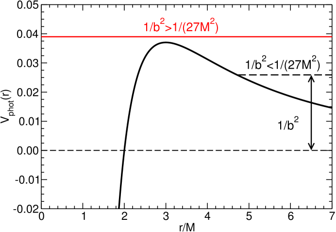
The motion of photons depends only on the impact parameter (as it should, by virtue of the equivalence principle: the same result can be obtained by a simple rescaling of the affine parameter [86]):
| (2.3.36) |
The potentials (2.3.34) and (2.3.35) are plotted in Figs. 2.1 and 2.2, respectively. The qualitative features of particle motion in these potentials are treated in most books on General Relativity (see e.g. [66, 45, 84, 22, 86]), so there is no need to repeat the discussion here, except for some important remarks in the next Section that will be useful below.
Note that, according to the definitions above, the derivatives of the radial particle potential and the derivatives of the potentials have opposite signs. Therefore unstable orbits (in particular the “light ring”, i.e. the unstable photon orbit at , for which ) have .
2.3.1 Circular Geodesics in the Schwarzschild Metric
By definition, circular geodesics have constant areal radius coordinate : and , with the second condition ensuring that circular orbits remain circular. From Eq. (2.2.28) it follows that . The condition is equivalent to
| (2.3.37) |
From this equality one can already draw two conclusions:
-
(i)
Circular geodesics exist only for .
-
(ii)
Null circular geodesics () exist only at .
The angular frequency of the circular orbit (as measured at infinity) is
| (2.3.38) |
Eq. (2.3.37) implies , and the condition translates to . Therefore we get the relativistic analog of Kepler’s law:
| (2.3.39) |
To understand the stability of these geodesics under small perturbations we must look at . After substituting from Eq. (2.3.37), we get
| (2.3.40) |
Thus,
-
(iii)
Circular geodesics with are stable (this is why is referred to as the “innermost stable circular orbit”, or ISCO).
-
(iv)
Circular geodesics with are all unstable.
2.3.2 The Critical Impact Parameter
The effective potential for geodesic motion was given in Eq. (2.3.30). Let us consider two extreme cases: and the ultrarelativistic limit (where the second case corresponds to massless, ultrarelativistic particles, and therefore it is equivalent to considering ).
For , i.e., particles dropped from rest at infinity, we have
From this factorization, it is clear that there is a turning point (i.e., a real value of for which ) if and only if . Furthermore, all turning points lie outside the horizon (that is located at ). It follows that the critical angular momentum for capture is
| (2.3.42) |
When we consider the capture of massless particles (), defining an impact parameter , we get
| (2.3.43) |
To find the turning points we must now solve a cubic equation. Following Chandrasekhar [23], we look for the critical such that the cubic polynomial has no real positive roots. Now, it is well known that the roots of the polynomial satisfy and . We know for sure that there is always one negative root, because the polynomial tends to as and it is positive (equal to ) at . Therefore we have two possibilities: (1) one real, negative root and two complex-conjugate roots, or (2) one real, negative root and two distinct, real roots. The critical case is when the two real roots of case (2) degenerate into a single real root. Clearly, at this point one must have
| (2.3.44) |
Substituting back into the polynomial, this will only be a root if
| (2.3.45) | |||||
| (2.3.46) |
The main conclusions of this discussion can be summarized as follows:
-
(1)
Circular null geodesics (the trajectories of massless scalars, photons or gravitons circling the black hole) are located at , and they are unstable;
-
(2)
The critical impact parameter for capture of light rays (or gravitons, or massless scalars) corresponds precisely to these circular null geodesics.
As we will see in Chapter 3, circular null geodesics are linked (in the geometric-optics limit) to the oscillation modes of black holes. To make this understanding quantitative, we need a measure of the instability rate of circular null geodesics. This measure relies on the classical theory of orbital stability based on Lyapunov exponents, that I review below.
2.4 Order and Chaos in Geodesic Motion
In the theory of dynamical systems, Lyapunov exponents are a measure of the average rate at which nearby trajectories converge or diverge in phase space. A positive Lyapunov exponent indicates a divergence between nearby trajectories, i.e., a high sensitivity to initial conditions. To investigate geodesic stability in terms of Lyapunov exponents, we begin with the equations of motion schematically written as
| (2.4.47) |
We linearize these equations about a certain orbit and we get
| (2.4.48) |
where
| (2.4.49) |
is the linear stability matrix [27]. The solution to the linearized equations can be written as
| (2.4.50) |
in terms of the evolution matrix , which must obey
| (2.4.51) |
as well as , so that Eq. (2.4.50) is satisfied at . The eigenvalues of are called “Lyapunov exponents”. More precisely, the principal Lyapunov exponent is the largest of these eigenvalues, such that
| (2.4.52) |
2.4.1 Lyapunov Exponents for Circular Orbits in Static, Spherically Symmetric Spacetimes
Let us now restrict attention to a class of problems for which one has a two dimensional phase space of the form . Let us focus on circular orbits in static, spherically symmetric metrics222Our treatment is actually general enough to study circular orbits in stationary spherically symmetric spacetimes, and also equatorial circular orbits in stationary spacetimes (including the higher-dimensional generalization of rotating black holes, known as the Myers-Perry metric): cf. [21] for generalizations to these cases.. and linearize the equations of motion with about orbits of constant areal radius . As pointed out by Cornish and Levin [27], Lyapunov exponents are in general coordinate-dependent. To measure the orbital instability rate through the principal Lyapunov exponent , a sensible choice is to use Schwarzschild time , i.e. the time measured by an observer at infinity. The relevant equations of motion are Eqs. (2.2.17) and (2.2.23). Linearizing them about circular orbits of radius yields
| (2.4.53) | |||
| (2.4.54) |
where dots denote derivatives with respect to , and it is understood that the quantities in the linearized equations must be evaluated at and . Converting from the affine parameter to Schwarzschild time (which implies dividing everything through by a factor ) we get the linear stability matrix
| (2.4.55) |
where
| (2.4.56) | |||||
| (2.4.57) |
Therefore, for circular orbits, the principal Lyapunov exponents can be expressed as
| (2.4.58) |
The fact that eigenvalues come in pairs is a reflection of energy conservation: the volume in phase space is also conserved [27]. From now on I will drop the sign, and simply refer to as the “Lyapunov exponent”.
From the equations of motion it follows that
| (2.4.59) |
where in the second equality I used Eq. (2.2.15). The definition of , Eq. (2.2.28), implies
| (2.4.60) |
and
| (2.4.61) |
so that finally
| (2.4.62) |
For circular geodesics [6], so Eq. (2.4.58) reduces to
| (2.4.63) |
and finally
| (2.4.64) |
Recall from our discussion of geodesics that unstable orbits have , and correspond to real values of the Lyapunov exponent . Following Pretorius and Khurana [79], we can introfuce a critical exponent
| (2.4.65) |
where was given in Eq. (2.3.38), and in addition we have introduced a typical orbital timescale and an instability timescale (note that in Ref. [27] the authors use a different definition of the orbital timescale, ). Then the critical exponent can be written as
| (2.4.66) |
For circular null geodesics in many spacetimes of interest [cf. Eq. (2.3.40)], which implies instability.
A quantitative characterization of the instability requires a calculation of the associated timescale . Let us turn to this calculation for timelike and circular orbits.
Timelike Geodesics
From Eq. (2.2.29), the requirement for circular orbits yields
| (2.4.67) |
where here and below all quantities are evaluated at the radius of a circular timelike orbit. Since the energy must be real, we require
| (2.4.68) |
The second derivative of the potential is
| (2.4.69) |
and the orbital angular velocity is given by
| (2.4.70) |
Using Eqs. (2.4.64), (2.2.25) and (2.4.69) to evaluate the Lyapunov exponent at the circular timelike geodesics, we get
| (2.4.71) | |||||
Bearing in mind that and that unstable orbits are defined by , we can see that will be real whenever the orbit is unstable, as expected.
Null Geodesics
Circular null geodesics satisfy the conditions:
| (2.4.72) | |||
| (2.4.73) |
and therefore
| (2.4.74) |
Here and below a subscript means that the quantity in question is evaluated at the radius of a circular null geodesic. An inspection of (2.4.74) shows that circular null geodesics can be seen as the innermost circular timelike geodesics. By taking another derivative and using Eq. (2.4.74) we find
| (2.4.75) |
and the coordinate angular velocity is
| (2.4.76) |
Let us define the “tortoise” coordinate
| (2.4.77) |
For circular orbits that satisfy Eq. (2.4.74), a simple calculation shows that
| (2.4.78) |
Combining this result with Eq. (2.4.75), we finally have
| (2.4.79) |
This is the main result of this Chapter. In the next Chapter I will show that the rate of divergence of circular null geodesics at the light ring, as measured by the principal Lyapunov exponent, is equal (in the geometrical optics limit) to the damping time of black-hole perturbations induced by any massless bosonic field.
Chapter 3 Waves
3.1 Massive Scalar Fields in a Spherically Symmetric Spacetime
Consider now the perturbations induced by a probe field (rather than a particle) propagating in a background spacetime, that for the purpose of this section could be either a black hole or a star. In the usual perturbative approach we assume that the scalar field contributes very little to the energy density (i.e. we drop quadratic terms in the field throughout, assuming that the energy-momentum tensor of the scalar field is negligible). Then the problem reduces to that of a scalar field evolving in a fixed background, and the “true” metric can be replaced by a solution to the Einstein equations, that we will assume for simplicity to be spherically symmetric. Let us therefore start from the metric (2.2.14), which reduces to the Schwarzschild metric when . The Klein-Gordon equation in this background reads
| (3.1.1) |
Here the mass has dimensions of an inverse length, (with ). The necessary conversions can be performed recalling that the Compton wavelength of a particle (in km) is related to its mass (in eV) by
| (3.1.2) |
Note also that a ten-Solar Mass black hole has a Schwarzschild radius of . Compton wavelengths comparable to the size of astrophysical black holes correspond to very light particles of mass eV (this observation will be useful in Chapter 4). Using a standard identity from tensor analysis, the Klein-Gordon equation can be written
| (3.1.3) |
where all quantities refer to the metric (2.2.14). Since the metric is spherically symmetric, the field evolution should be independent of rotations: this suggests that the angular variables and should factor out of the problem. The field can be decomposed as
| (3.1.4) |
where the superscript “” is a reminder that these are spin-zero perturbations, are the usual scalar spherical harmonics, and the associated Legendre functions satisfy
| (3.1.5) |
Note that this decomposition is the most general possible, because the spherical harmonics are a complete orthonormal set of functions. Inserting (3.1.4) into equation (3.1.3) and using (3.1.5), we get the following radial wave equation for :
| (3.1.6) |
where we can write rather than because the differential equation does not depend on (the background is spherically symmetric). In analogy with (2.4.77), we can introduce the “generalized tortoise coordinate”
| (3.1.7) |
to eliminate the first-order derivative and obtain the following radial equation:
| (3.1.8) |
where the mass-dependent scalar potential reads
| (3.1.9) |
The tortoise coordinate will turn out to be useful because, in the Schwarzschild metric, the location of the horizon () corresponds to , so the problem of black-hole perturbations can be formulated as a one-dimensional scattering problem over the real axis.
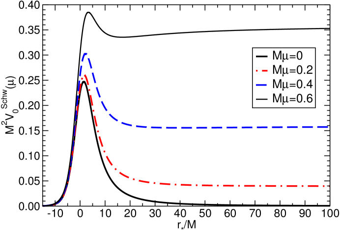
For most black-hole metrics of interest, . In particular, for the Schwarzschild metric the potential reads
| (3.1.10) |
and the tortoise coordinate satisfies
| (3.1.11) |
which is easily integrated to give
| (3.1.12) |
where the integration constant has been fixed using a common choice in the literature. The potential (3.1.10) has some crucial properties that are illustrated in Fig. 3.1: (i) it tends to zero as (), where ; (ii) it tends to as (), so whenever there is a “reflective potential barrier” at infinity; (iii) when the mass term is nonzero there is a local minimum outside the peak of the potential, that allows for the existence of quasi-bound states (that slowly leak out to infinity because of dissipation).
 |
-
Box 3.1 Master Equation for Massless Bosonic Fields, and the Peak of the Potential
Separating the equations describing massless spin-one and spin-two (i.e., electromagnetic and gravitational) perturbations in the Schwarzschild background is not as easy as separating the angular dependence for the scalar field (things get even harder for massive fields: see references in Section 4.2 below). The angular separation can be performed using vector and tensor spherical harmonics (see e.g. [81, 97]), and it leads to a remarkable result: perturbations induced by any of these bosonic fields satisfy a single “master equation”,
(3.1.13) where
(3.1.14) In the last line we set to simplify the algebra. We also introduced and , where is the spin of the perturbing field. Then Eq. (3.1.10) is just a special case for and . Let us look for the extrema of the function . It is easy to show that
(3.1.15) Besides the asymptote as , the only zero occurs when the curly brace vanishes. Multiplying the curly brace by one gets a quadratic equation, that is easily solved for the location of the extremum:
(3.1.16) It is readily seen that when (i.e. in the eikonal, or geometric optics, limit). Even for small ’s the location of the peak is very close to the marginal photon orbit: for , one gets ; for , one gets .
3.2 Solution of the Scattering Problem
Unlike most idealized macroscopic physical systems, perturbed black-hole spacetimes are intrinsically dissipative due to the presence of the event horizon, which acts as a one-way membrane. In fact, the system is “leaky” both at the horizon and at infinity, where energy is dissipated in the form of gravitational radiation. This precludes a standard normal-mode analysis: dissipation means that the system is not time-symmetric, and that the associated boundary-value problem is non-Hermitian. In general, after a transient that depends on the source of the perturbation, the response of a black hole is dominated by characteristic complex frequencies (the “quasinormal modes”, henceforth QNMs). The imaginary part is nonzero because of dissipation, and its inverse is the decay timescale of the perturbation. The corresponding eigenfunctions are usually not normalizable, and, in general, they do not form a complete set (cf. [25, 72] for more extensive discussions). Almost any real-world physical system is dissipative, so one might reasonably expect QNMs to be ubiquitous in physics. QNMs are indeed useful in the treatment of many dissipative systems, e.g. in the context of atmospheric science and leaky resonant cavities. Extensive reviews on black-hole QNMs and their role in various fields of physics (including gravitational-wave astronomy, the gauge-gravity duality and high-energy physics) can be found in [71, 56, 12, 57].
Black-hole QNMs were initially studied to assess the stability of the Schwarzschild metric [93, 77]. Goebel [40] was the first to realize that they can be thought of as waves traveling around the black hole: more precisely, they can be interpreted as waves trapped at the unstable circular null geodesic (the “light ring”) and slowly leaking out. This qualitative picture was refined by several authors over the years [36, 63, 91, 32, 21, 31, 35]. It will be shown below that the instability timescale of the geodesics is the decay timescale of the QNM, and the oscillation frequency , with the speed of light and the light-ring radius (see [21] for generalizations of these arguments to rotating and higher-dimensional black holes).
One of the most fascinating aspects of black-hole physics is that the master equation (3.1.13) can be solved using methods familiar from nonrelativistic quantum mechanics, in particular from scattering theory. We will first review a method developed by Leaver [59] to compute QNM frequencies “exactly” (within the limits of a computer’s numerical accuracy). Leaver’s method follows quite closely techniques that were developed to deal with the hydrogen ion in quantum mechanics as early as 1934 [52]. Then we will confirm the intuitive picture of black-hole QNMs as light-ring perturbation using one of the simplest “textbook” approximation technique to solve scattering problems: the Wentzel-Kramers-Brillouin (WKB) approximation. In the black-hole perturbation theory context, the WKB approximation was first investigated by Mashhoon [62], Schutz and Will [85].
3.2.1 Leaver’s Solution
Leaver’s solution of the wave equation is based on a classic 1934 paper by Jaffé on the electronic spectra of the hydrogen molecular ion [52] – quantum mechanics comes to the rescue again! The wave equation is found to be a special case of the so-called “generalized spheroidal wave equation” [60], for which the solution can be written as a series expansion. By replacing the series expansion into the differential equations and imposing QNM boundary conditions, one finds recursion relations for the expansion coefficients. The series solution converges only when a certain continued fraction relation involving the mode frequency and the black hole parameters holds. The evaluation of continued fractions amounts to elementary algebraic operations, and the convergence of the method is excellent, even at high damping. In the Schwarzschild case, in particular, the method can be tweaked to allow for the determination of modes of order up to [70].
As stated (without proof) in Box 3.1, the angular dependence of the metric perturbations of a Schwarzschild black hole can be separated using tensorial spherical harmonics [97]. Depending on their behavior under parity transformations, the perturbation variables are classified as polar (even) or axial (odd). The resulting differential equations can be manipulated to yield two wave equations, one for the polar perturbations (that we shall denote by a “plus” superscript) and one for the axial perturbations (“minus” superscript):
| (3.2.17) |
We are interested in solutions of equation (3.2.17) that are purely outgoing at spatial infinity () and purely ingoing at the black hole horizon (). These boundary conditions are satisfied by an infinite, discrete set of complex frequencies (the QNM frequencies). For the Schwarzschild solution the two potentials are quite different, yet the QNMs for polar and axial perturbations are the same. The proof of this suprising fact can be found in [23]. The underlying reason is that polar and axial perturbations are related by a differential transformation discovered by Chandrasekhar [23], and both potentials can be seen to emerge from a single “superpotential”. In fancier language, the axial and polar potentials are related by a supersymmetry transformation (where “supersymmetry” is to be understood in the sense of nonrelativistic quantum mechanics): cf. [61]. Since polar and axial perturbations are isospectral and has an analytic expression which is simpler to handle, we can focus on the axial equation for , i.e. the master equation (3.1.13) with .
We will now find an algebraic relation that can be solved (numerically) to determine the eigenfrequencies of scalar, electromagnetic and gravitational perturbations of a Schwarzschild black hole. For a study of the differential equation it is convenient to use units where , so that the horizon is located at (we will only use these units in this section). The tortoise coordinate and the usual Schwarzschild coordinate radius are related by
| (3.2.18) |
with . When written in terms of the “standard” radial coordinate and in units , the master equation (3.1.13) reads:
| (3.2.19) |
where is the spin of the perturbing field ( for scalar, electromagnetic and gravitational perturbations, respectively) and is the angular index of the perturbation. Perturbations of a Schwarzschild background are independent of the azimuthal quantum number , because of spherical symmetry (this is not true for Kerr black holes). Equation (3.2.19) can be solved using a series expansion of the form:
| (3.2.20) |
where the prefactor is chosen to incorporate the QNM boundary conditions at the horizon and at infinity:
| (3.2.21) | |||
| (3.2.22) |
Substituting the series expansion (3.2.20) in (3.2.19) we get a three term recursion relation for the expansion coefficients :
| (3.2.23) | |||
where , and are simple functions of the frequency , and [59]:
| (3.2.24) | |||
| (3.2.25) | |||
| (3.2.26) |
A mathematical theorem due to Pincherle guarantees that the series is convergent (and the QNM boundary conditions are satisfied) when the following continued fraction condition on the recursion coefficients holds:
| (3.2.27) |
The –th QNM frequency is (numerically) the most stable root of the –th inversion of the continued-fraction relation (3.2.27), i.e., it is a solution of
The infinite continued fraction appearing in equation (3.2.1) can be summed “bottom to top” starting from some large truncation index . Nollert [70] has shown that the convergence of the procedure improves if the sum is started using a wise choice for the value of the “rest” of the continued fraction, , defined by the relation
| (3.2.28) |
Assuming that the rest can be expanded in a series of the form
| (3.2.29) |
it turns out that the first few coefficients in the series are , , and (the latter coefficient contains a typo in [70], but this is irrelevant for numerical calculations).
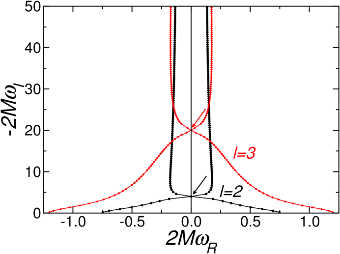
The dominant QNM frequencies with and resulting from this procedure are shown in Table 3.1 and Figure 3.2. Reintroducing physical units, the fundamental oscillation frequency and the damping time of an astrophysical black hole scale with mass according to the relation
| (3.2.30) |
An “algebraically special” mode, whose frequency is (almost) purely imaginary, separates the lower QNM branch from the upper branch [24]. This algebraically special mode is located at
| (3.2.31) |
and it can be taken as roughly marking the onset of the asymptotic high-damping regime. The algebraically special mode quickly moves downwards in the complex plane (i.e., upwards in the figure) as increases: from Table 3.1 we see that it corresponds to an overtone index when , and to an overtone index when . This means that for high values of the asymptotic high-damping regime sets in later, becoming harder to probe using numerical methods. The algebraically special modes are a fascinating technical subject: they can be shown to be related to the instability properties of naked singularities [18], and (strictly speaking) they are not even QNMs, because they do not satisify QNM boundary conditions: see e.g. [8] and references therein.
| n | ||
|---|---|---|
| 1 | (0.747343,-0.177925) | (1.198887,-0.185406) |
| 2 | (0.693422,-0.547830) | (1.165288,-0.562596) |
| 3 | (0.602107,-0.956554) | (1.103370,-0.958186) |
| 4 | (0.503010,-1.410296) | (1.023924,-1.380674) |
| 5 | (0.415029,-1.893690) | (0.940348,-1.831299) |
| 6 | (0.338599,-2.391216) | (0.862773,-2.304303) |
| 7 | (0.266505,-2.895822) | (0.795319,-2.791824) |
| 8 | (0.185617,-3.407676) | (0.737985,-3.287689) |
| 9 | (0.000000,-3.998000) | (0.689237,-3.788066) |
| 10 | (0.126527,-4.605289) | (0.647366,-4.290798) |
| 11 | (0.153107,-5.121653) | (0.610922,-4.794709) |
| 12 | (0.165196,-5.630885) | (0.578768,-5.299159) |
| 20 | (0.175608,-9.660879) | (0.404157,-9.333121) |
| 30 | (0.165814,-14.677118) | (0.257431,-14.363580) |
| 40 | (0.156368,-19.684873) | (0.075298,-19.415545) |
| 41 | (0.154912,-20.188298) | (-0.000259,-20.015653) |
| 42 | (0.156392,-20.685630) | (0.017662,-20.566075) |
| 50 | (0.151216,-24.693716) | (0.134153,-24.119329) |
| 60 | (0.148484,-29.696417) | (0.163614,-29.135345) |
Nollert was the first to compute highly damped quasinormal frequencies corresponding to gravitational perturbations [70]. His main result was that the real parts of the quasinormal frequencies are well fitted, for large , by a relation of the form
| (3.2.32) |
These numerical results are perfectly consistent with analytical calculations [13]. Motl [68] analyzed the continued fraction condition (3.2.27) to find that highly damped quasinormal frequencies satisfy the relation
| (3.2.33) |
(in units , the Hawking temperature of a Schwarzschild black hole ). This conclusion was later confirmed by complex-integration techniques [69] and phase-integral methods [3], and it may have a connection with Bekenstein’s ideas on black-hole area quantization [47].
3.2.2 The WKB Approximation
While Leaver’s method provides the most accurate numerical solution of the scattering problem, the WKB approximation is useful to develop physical intuition on the meaning of QNMs. The derivation below follows quite closely the paper by Schutz and Will [85], which in turn is based on the excellent treatment in the book by Bender and Orszag [7]. Consider the equation111In quantum mechanics, the Schrödinger equation for a particle of mass and energy moving in a one-dimensional potential (3.2.34) can be rewritten in the previous form with (3.2.35)
| (3.2.36) |
where is the radial part of the perturbation variable (the time dependence has been separated by Fourier decomposition, and the angular dependence is separated using the scalar, vector or tensor spherical harmonics appropriate to the problem at hand). The coordinate is a tortoise coordinate such that at the horizon and at spatial infinity. The function is constant in both limits () but not necessarily the same at both ends, and it rises to a maximum in the vicinity of (more specifically, as we have seen above, at ). Since tends to a constant at large , we have
| (3.2.37) |
with . If , . With our convention on the Fourier decomposition (), outgoing waves at correspond to the positive sign in the equation above, and waves going into the horizon as correspond to the negative sign in the equation above (cf. Fig. 3.1).
The domain of definition of can be split in three regions: a region I to the left of the turning point where , a “matching region” II with , and a region III to the right of the turning point where . As shown in Box 3.2.2, in regions I and III we can write the solution in the “physical optics” WKB approximation:
| (3.2.38) | |||
| (3.2.39) |
-
Box 3.2 WKB Approximation: “Physical Optics”
Introduce a perturbative parameter (proportional to in quantum mechanics) and write the ODE as
(3.2.40) Now write the solution in the form
(3.2.41) and compute the derivatives:
(3.2.42) (3.2.43) Substituting into the ODE and dividing by the common exponential factors we get
(3.2.45) The first two terms in the expansion yield the so-called “eikonal equation” and “transport equation”:
(3.2.46) (3.2.47) The solution to the eikonal equation is
(3.2.48) while the solution to the transport equation is
(3.2.49) The leading-order solution is called the “geometrical optics” approximation. The next-to-leading order solution (including ) is called the “physical optics” approximation. For higher-order solutions, cf. [7, 50, 58].
The idea is now to find the equivalent of the Bohr-Sommerfeld quantization rule from quantum mechanics. We want to relate two WKB solutions across the “matching region” whose limits are the classical turning points, where . The technique works best when the classical turning points are close, i.e. when , where is the peak of the potential. In region II, we expand
| (3.2.50) |
If we set and we make the change of variables , we find that the equation reduces to
| (3.2.51) |
We now define a parameter such that
| (3.2.52) |
Then the differential equation takes the form
| (3.2.53) |
whose solutions are parabolic cylinder functions, commonly denoted by [1, 7]. These special functions are close relatives of Hermite polynomials (this makes sense, because the quadratic approximation means that we locally approximate the potential as a quantum harmonic oscillator problem, and Hermite polynomials are well known to be the radial solutions of the quantum harmonic oscillator). The solution in region II is therefore a superposition of parabolic cylinder functions:
| (3.2.54) |
Using the asymptotic behavior of parabolic cylinder functions [1, 7] and imposing the outgoing-wave condition at spatial infinity we get, near the horizon,
| (3.2.55) |
QNM boundary conditions imply that the outgoing term, proportional to , should be absent, so , or . Therefore the leading-order WKB approximation yields a “Bohr-Sommerfeld quantization rule” defining the QNM frequencies:
| (3.2.56) |
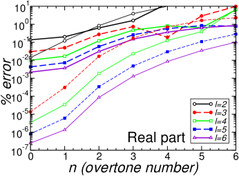
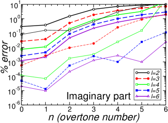
Higher-order corrections to this parabolic approximation have been computed [77]. Iyer and Will [50, 49] carried out a third-order WKB expansion, and Konoplya [58] pushed the expansion up to sixth order. There is no rigorous proof of convergence, but the results do improve for higher WKB orders. Fig. 3.3 compares numerical results for the QNMs of Schwarzschild black holes from Leaver’s continued fraction method against third-order (thick lines) and sixth-order (thin lines) WKB predictions. The WKB approximation works best for low overtones, i.e. modes with a small imaginary part, and in the eikonal limit of large (which corresponds to large quality factors, or large ). The method assumes that the potential has a single extremum, which is the case for most (but not all) black-hole potentials: see e.g. [48] for counterexamples.
 |
 |
3.3 Geodesic Stability and Black-Hole Quasinormal Modes
Let us reconsider the Bohr-Sommerfeld quantization condition (3.2.56). In a spherically symmetric, asymptotically flat spacetime of the form (2.2.14), the Klein-Gordon equation can be written as in Eq. (3.2.36) with the tortoise coordinate (2.4.77). In the eikonal limit () we get
| (3.3.57) |
It is easy to check that scalar, electromagnetic and gravitational perturbations of static black holes have the same behavior in the eikonal limit (in fact, the same conclusion applies to higher-dimensional spacetimes [53, 48, 54]). In other words, there is a well-defined geometric-optics (eikonal) limit where the potential for a wide class of massless perturbations is “universal”. For in Eq. (3.3.57) above we find that the extremum of satisfies , i.e. coincides with the location of the null circular geodesic , as given by Eq. (2.4.74). Furthermore, the WKB formula (3.2.56) implies that, in the large- limit,
| (3.3.58) |
Comparing this result with Eqs. (2.4.76) and (2.4.79), it follows that
| (3.3.59) |
This is one of the punchlines of these notes: in the eikonal approximation, the real and imaginary parts of the QNMs of any spherically symmetric, asymptotically flat spacetime are given by (multiples of) the frequency and instability timescale of the unstable circular null geodesics.
Dolan and Ottewill [35] have introduced a WKB-inspired asymptotic expansion of QNM frequencies and eigenfunctions in powers of the angular momentum parameter . Their asymptotic expansion technique is easily iterated to high orders, and it is very accurate (at least for spherically symmetric spacetimes). The asymptotic expansion also provides physical insight into the nature of QNMs, nicely connecting the geometrical understanding of QNMs as perturbations of unstable null geodesics with the singularity structure of the Green’s function.
3.4 Superradiant Amplification
The discussion so far was limited to uncharged and/or nonrotating black holes. The inclusion of charge and rotation leads to the interesting possibility of superradiant amplification. I will first explain the conceptual foundations of superradiance, and then look at the astrophysically most interesting case of rotational superradiance in the Kerr spacetime. For a stationary, asymptotically flat black hole, the equations describing spin- fields can be written in the form
| (3.4.60) |
where as usual is the frequency in a Fourier transform with respect to the asymptotic time coordinate: , and the radius is a convenient tortoise coordinate. As it turns out, the tortoise coordinate and the radial potential at the horizon () and at infinity () behave as follows:
| (3.4.61) |
where is a positive constant. The function can be related to rotation (in the Kerr geometry , with an azimuthal number and the angular velocity of the horizon) or it can be a “chemical potential” (in the Reissner-Nordström geometry , where is the charge of the perturbing field and the charge of the black hole).
Waves scattering in this geometry have the following asymptotic behavior:222For simplicity, here we consider a massless field, but the discussion is generalized to massive fields in a straightforward way.
| (3.4.62) |
These boundary conditions correspond to an incident wave of unit amplitude coming from infinity, giving rise to a reflected wave of amplitude going back to infinity. At the horizon there is a transmitted wave of amplitude going into the horizon, and a wave of amplitude going out of the horizon.
Assuming a real potential (this is true for massive scalar fields and in most other cases), the complex conjugate of the solution satisfying the boundary conditions (3.4.62) will satisfy the complex-conjugate boundary conditions:
| (3.4.63) |
These two solutions are linearly independent, and the standard theory of ODEs implies that their Wronskian is a constant (independent of ). If we evaluate the Wronskian near the horizon, we get
| (3.4.64) |
and near infinity we find
| (3.4.65) |
where we used . Equating the two yields
| (3.4.66) |
The reflection coefficient is usually less than unity, but there are some notable exceptions:
-
•
If , i.e., if there is no absorption by the black hole, then .
-
•
If , i.e., if the hole absorbs more than what it gives away, there is superradiance in the regime . Indeed, for we have that . Such a scattering process, where the reflected wave has actually been amplified, is known as superradiance. Of course the excess energy in the reflected wave must come from energy “stored in the black hole”, which therefore decreases.
-
•
If , there is superradiance in the other regime, but this condition also means that there is energy coming out of the black hole, so it is not surprising to see superradiance.
For the Schwarzschild spacetime , and only waves going into the horizon are allowed (). Therefore
| (3.4.67) |
This is simply summarized by saying that energy is conserved.
If we impose the physical requirement that no waves should come out of the horizon () and we set , as appropriate for superradiance in the Kerr metric, we get
| (3.4.68) |
Therefore superradiance in the Kerr spacetime will occur whenever
| (3.4.69) |
The amount of superradiant amplification depends on the specific field perturbing the black hole, and it must be obtained by direct integration of the wave equation.
There is no superradiance for fermions: can you tell why?
3.4.1 Massive Scalar Fields in the Kerr Metric
As a prototype of the general treatment of superradiance provided above, consider the Klein-Gordon equation (3.1.1) describing massive scalar field perturbations in the Kerr metric. In Boyer-Lindquist coordinates, the equation reads (see e.g. [34])
| (3.4.70) | |||
where , and we assumed an azimuthal dependence . The black-hole inner and outer horizons are located at the zeros of , namely . Focus for simplicity on the case . Assuming a harmonic time dependence and using spheroidal wave functions [37, 9] to separate the angular dependence,
| (3.4.71) |
leads to the radial wave equation
| (3.4.72) |
where
| (3.4.73) | |||
| (3.4.74) | |||
| (3.4.75) |
is an angular separation constant, equal to when and obtained in more complicated ways when [9].
We can easily see that this potential satisfies the boundary conditions (3.4.61) for superradiance. As , , , , , , and therefore the potential .
As , , . Therefore , , and the dominant term is
| (3.4.76) |
Now, the previous treatment implies that
| (3.4.77) |
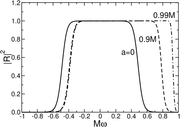
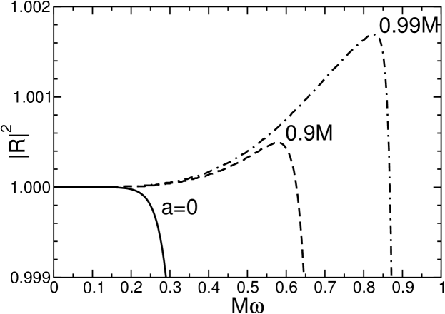
The superradiant amplification for scalar perturbations with is shown in Fig. 3.4 (where I reproduce the results obtained in [4] by an independent frequency-domain numerical code). As a general rule, superradiant instabilities get stronger as the spin of the perturbing field increases.
Chapter 4 The Unreasonable Power of Perturbation Theory: Two Examples
4.1 Critical Phenomena in Binary Mergers
The theory of Lyapunov exponents (Section 2.4) has fascinating applications in the study of critical phenomena in black-hole binaries. In the encounter of two black holes, three outcomes are possible: scattering for large values of the impact parameter of the collision; merger for small values of the impact parameter; and a delayed merger in an intermediate regime, where the black holes can revolve around each other (in principle) an infinite number of times by fine-tuning the impact parameter around some critical value .
I will illustrate this possibility by first considering the simple case of extreme mass-ratio binaries (i.e., to a first level of approximation, point particles moving along geodesics in a black-hole spacetime), and then by reporting results from numerical simulations of comparable-mass black hole binary encounters.
4.1.1 Extreme Mass-Ratio Binaries
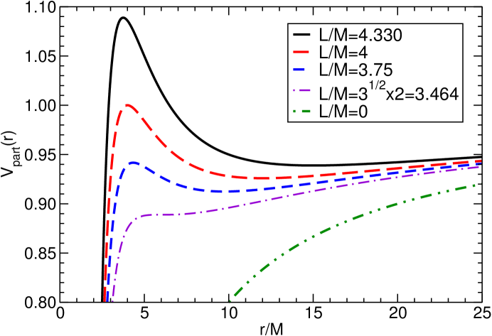
Consider equatorial () timelike geodesic in the Schwarzschild background. From Eqs. (2.2.25), (2.2.26) and (2.3.30) with we have
| (4.1.1) | |||||
| (4.1.2) | |||||
| (4.1.3) |
where , we used the definition (2.3.34) for timelike particles, and (as usual) dots stand for derivatives with respect to proper time . Recall that is the particle’s energy at infinity per unit mass , so corresponds to an infall from rest and the limit corresponds to ultrarelativistic motion.
Geodesics can be classified according to how their energy compares to the maximum value of the effective potential (2.3.34). A simple calculation shows that the maximum is located at
| (4.1.4) |
and that the potential at the maximum has the value
| (4.1.5) |
The scattering threshold is then defined by the condition : orbits with are captured, while those with are scattered. Given some , the critical radius or impact parameter that defines the scattering threshold is obtained by solving the scattering threshold condition (in general, numerically) to obtain , and then using the following definition of the impact parameter
| (4.1.6) |
to obtain .
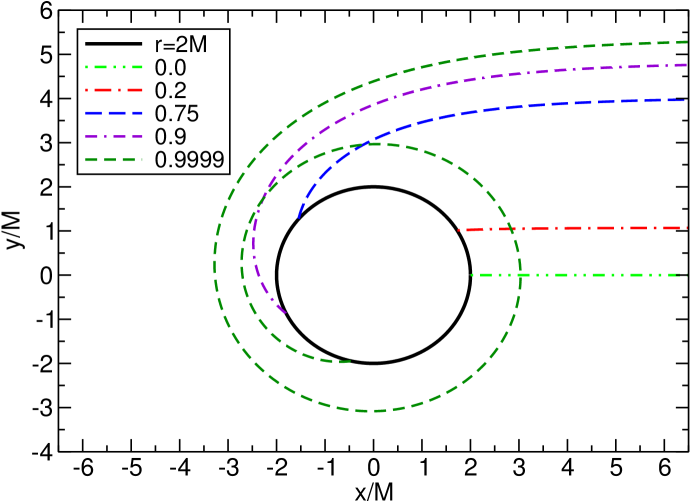
The geodesic equations listed above can be integrated numerically for chosen values of and . For the particle does not plunge, but rather scatters to infinity. Examples of plunging orbits for and different angular momenta (i.e., different impact parameters) are shown in Fig. 4.1 in Cartesian-like coordinates , . The number of revolutions around the black hole before plunge increases as .
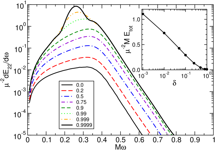
Using black-hole perturbation theory, it is possible to compute the energy radiated by particles falling into the black hole with different values of . The details of the calculation can be found in [11] and references therein. In the frequency domain, the radiated energy can be decomposed as a sum
| (4.1.7) |
where the indices refer to the angular functions used to separate variables (here spin-weighted spherical harmonics of spin weight two). The dominant contribution to the radiation comes from modes with . Figure 4.2 shows the energy spectrum of the mode for a particle with (infall from rest) and different values of the orbital angular momentum . For the energy spectra show a simple structure, first identified for radial infalls () in [29]: the spectrum vanishes at low frequencies, it has a peak, and then an exponential decay at frequencies larger than the black hole’s fundamental quasinormal mode frequency for the given . However, additional features appear when grows, and the nature of the spectra changes quite significantly as . As shown in Fig. 4.2, as we fine-tune the angular momentum to the critical value separating plunge and scattering the energy spectra with clearly display a second peak, which is related to the orbital motion of the particle. This very distinctive “bump” appears at a frequency slightly lower than the quasinormal mode frequency, significantly enhancing the radiated energy. The location of the “bump” corresponds to (twice) the orbital frequency of the particle at the marginally bound orbit, i.e. . The reason for this local maximum in the spectrum is that when the particle orbits a large number of times close to the circular marginally bound orbit with radius (here because ), eventually taking an infinite amount of proper time to reach the horizon. The proximity of the orbit to criticality is conveniently described by a small dimensionless “criticality parameter”
| (4.1.8) |
In the limit , how many times does the particle hover at the marginally bound circular geodesics before plunging? The answer is given by the Lyapunov exponent calculation of Chapter 2 (see e.g. [79]). To linear order, the growth of the perturbation around the marginally bound orbit is described by
| (4.1.9) |
so . Perturbation theory breaks down when , and by that time the number of orbits that have been completed is . Furthermore, (with some constant) for geodesics approaching the marginally bound orbit. Taking the natural logarithm of (4.1.9) and substituting these relations yields
| (4.1.10) |
Now recall our result (2.4.64) for the Lyapunov exponent to get:
| (4.1.11) |
Therefore the particle orbits the black hole
| (4.1.12) |
times before plunging [10] (recall that dots stand for derivatives with respect to proper time). This logarithmic scaling with the “criticality parameter” is typical of many phenomena in physics (see e.g. [26] for the discovery that critical phenomena occur in gravitational collapse, and [44] for a review of subsequent work in the field).
For the Schwarzschild effective potential, , and the angular velocity is nothing but evaluated at the marginally bound orbit . When the marginally bound orbit is located at , and
| (4.1.13) |
The inset of Fig. 4.2 shows that the total radiated energy in the limit does indeed scale logarithmically with , and hence linearly with the number of orbits , as expected from Eq. (4.1.13) for radiation from a particle in circular orbit at the marginally bound geodesic.
In the ultrarelativistic limit the marginally bound orbit is located at the light ring , the corresponding orbital frequency and
| (4.1.14) |
As argued in Chapter 3, the orbital frequency at the light ring is intimately related with the eikonal (long-wavelength) approximation of the fundamental quasinormal mode frequency of a black hole (see also [77, 63, 14, 21]). This implies that ultrarelativistic infalls with near-critical impact parameter are in a sense the most “natural” and efficient process to resonantly excite the dynamics of a black hole. The proper oscillation modes of a Schwarzschild black hole cannot be excited by particles on stable circular orbits (i.e. particles with orbital radii in Schwarzschild coordinates), but near-critical ultrarelativistic infalls are such that the orbital “bump” visible in Figure 4.2 moves just slightly to the right to overlap with the “knee” due to quasinormal ringing. So ultrarelativistic infalls have just the right orbital frequency to excite black hole oscillations.
4.1.2 Comparable-Mass Binaries
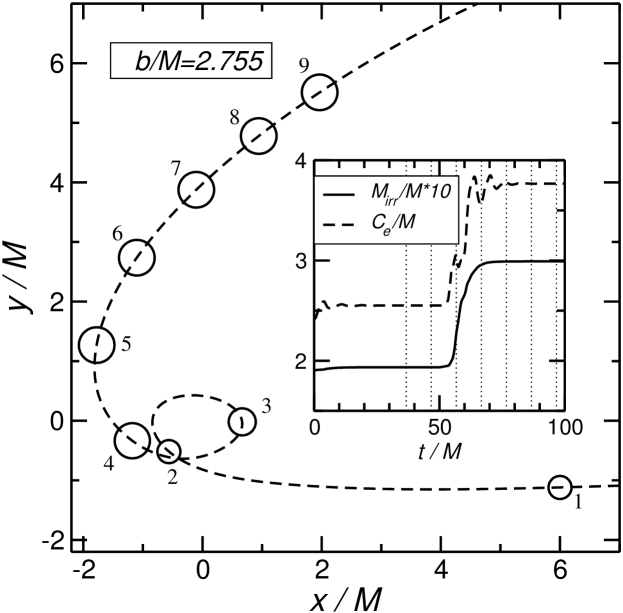
Pretorius and Khurana [79] demonstrated that critical behavior of the kind shown above, where the number of orbits scales logarithmically with some criticality parameter , occurs also in the encounters of comparable-mass black hole mergers. Now the question is: suppose that two comparable-mass black holes collide close to the speed of light, so that all the center-of-mass energy of the system is kinetic energy. Is it possible to radiate all of the energy of the system by fine-tuning the impact parameter near threshold? And if so, what is the final state of the collision? As demonstrated by numerical relativity simulations in a series of papers [89, 90, 88], the answer to this question is “no”, and the reason is that the black holes absorb a significant fraction of the energy during a close encounter.
The encounter of two equal-mass black holes is illustrated in Fig. 4.3 (from [88]). The plot shows the trajectory of one of the two black holes (the trajectory of the other hole is reflection-symmetric with respect to that of the first hole). In the numerical simulations we monitor the apparent horizon dynamics of the individual holes by measuring the equatorial circumference and the irreducible mass of each black hole before and after the encounter. The inset of the right panel of Fig. 4.3 shows the variation of these quantities with time: absorption occurs over a short timescale . Since the apparent horizon area , in this way we can estimate the rest mass and dimensionless spin of each hole before (, ) and after (, ) the first encounter. We define the absorbed energy . It turns out that accounts for most of the total available kinetic energy in the system, and therefore the system is no longer kinetic-energy dominated after the encounter. A fit of the data yields and , where is the Lorentz boost parameter, suggesting that radiation and absorption contribute about equally in the ultrarelativistic limit, and therefore that absorption sets an upper bound on the maximum energy that can be radiated.
The fact that absorption and emission are comparable in the ultrarelativistic limit is supported by point-particle calculations in black hole perturbation theory. For example, Misner et al. [65] studied the radiation from ultrarelativistic particles in circular orbits near the Schwarzschild light ring, i.e. at . Using a scalar-field model they found that 50% of the radiation is absorbed and 50% is radiated as . The same conclusion applies to gravitational perturbations of Schwarzschild black holes when one ignores radiation reaction (self-force) effects, and a recent analysis including self-force effects finds that of the energy should be absorbed by nonrotating black holes as (cf. Fig. 4 of [43]).
4.2 Black-Hole Bombs
The superradiant amplification mechanism discussed in Section 3.4 has a rather dramatic consequence for astrophysics and particle physics: measurements of the spin of massive black holes, the largest and simplest macroscopic objects in the Universe, can be used to set upper bounds on the mass of light bosonic particles. The reason behind this striking connection between the smallest and largest objects in our physical world is the so-called “black-hole bomb” instability first investigated by Press and Teukolsky [78] (see also [20], and [87] for a recent rigorous proof for scalar perturbations).
The idea is the following. Imagine surrounding a rotating black hole by a perfectly reflecting mirror. An ingoing monochromatic wave with frequency in the superradiant regime defined by Eq. (3.4.69) will be reflected and amplified at the expense of the rotational energy of the black hole, then it will be reflected again by the mirror and amplified once more. The process keeps repeating and triggers a runaway growth of the perturbation – a “black-hole bomb”. The end state cannot be predicted in linearized perturbation theory, but it is reasonable to expect that we will be left with a slowly rotating (or nonrotating) black hole, transferring the whole rotational energy of the hole (a huge amount compared to nuclear physics standards!) to the field.
The original Press-Teukolsky mechanism is of mostly speculative interest: for example, one could imagine a very advanced civilization building perfectly reflective mirrors around rotating black holes to solve their energy problems. Luckily, Nature gives us actual “mirrors” in the form of massive bosonic fields. As shown in Fig. 3.1 for massive scalars, whenever the field has mass the effective potential for wave propagation tends to a nonzero value at infinity. This potential barrier is the particle-physics analog of Press and Teukolsky’s perfectly reflecting mirror.
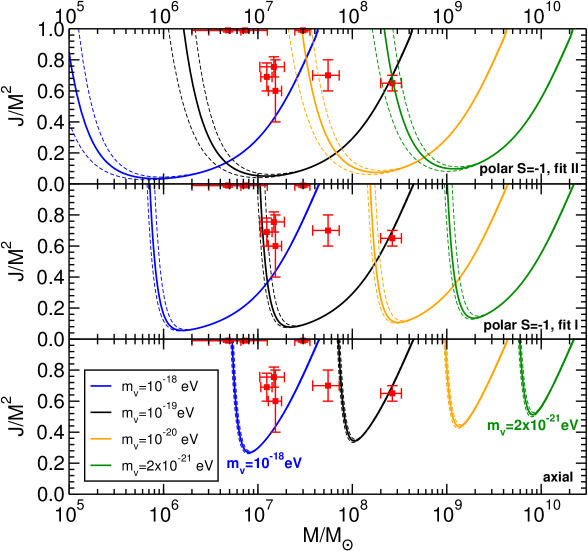
This simple consideration has immediate implications for fundamental physics. Many proposed extensions of the Standard Model predicted the existence of ultralight bosons, such as the light scalars with of the “string axiverse” scenario [5], “hidden photons” [41, 42, 51, 17] and massive gravitons [41, 46, 30]. Explicit calculations of the instability timescales have been performed for massive scalar [78, 28, 98, 33, 34, 80, 19], vector (Proca) [73, 74] and tensor (massive graviton) [16] perturbations of a Kerr black hole. In all cases the instability is regulated by the dimensionless parameter (in units ), where is the BH mass and is the bosonic field mass, and it is strongest for maximally spinning BHs when . As discussed around Eq. (3.1.2), for a solar-mass black hole and a field of mass eV the parameter . In this case the instability is exponentially suppressed [98], and the instability timescale would be larger than the age of the Universe. The strongest superradiant instabilities develop when , i.e. when the Compton wavelength of the perturbing field is comparable to the “size” of the black hole’s event horizon. This can occur for light primordial BHs that may have been produced in the early Universe, or for the ultralight exotic particles proposed in some extensions of the Standard Model. In particular, fields of mass eV around the heaviest supermassive black holes () are ideal candidates.
This yields stringent constraints on the mass of the perturbing field. If there were fields of mass around a supermassive rotating black hole, the superradiant instability would reduce their spin on a timescale that can be computed using black-hole perturbation theory (this timescale is shortest when ). We can exclude the existence of a field of mass whenever the superradiant instability timescale is smaller than the Salpeter time, i.e. the typical time over which accretion could potentially spin up the hole [82]. By setting the Salpeter timescale equal to the instability timescale we can draw “instability windows” such as those shown in Fig. 4.4; these are sometimes called gaps in the mass-spin black-hole “Regge spectrum” [5]. Any measurement of a black-hole spin with value above one of the instability windows excludes a whole range of masses for the perturbing field.
It is worth mentioning that massive fields can have other potentially observable signatures. They can modify the inspiral dynamics of compact binaries [2] and even freeze the inspiral of compact objects into massive black holes, creating “floating orbits” that produce stimulated emission of radiation by extracting the hole’s rotational energy (the gravitational-wave equivalent of a laser!) [19, 96]. Another potentially observable event is a “bosenova”, i.e. a collapse of the axion cloud producing a relatively large emission of scalar radiation (see e.g. [55, 95, 67, 94]).
Bibliography
- [1] M. Abramowitz and I. A. Stegun. Handbook of Mathematical Functions with Formulas, Graphs, and Mathematical Tables. Dover, New York, 1972.
- [2] J. Alsing, E. Berti, C. M. Will, and H. Zaglauer. Gravitational radiation from compact binary systems in the massive Brans-Dicke theory of gravity. Phys.Rev., D85:064041, 2012.
- [3] N. Andersson and C. J. Howls. The asymptotic quasinormal mode spectrum of non-rotating black holes. Class. Quant. Grav., 21:1623–1642, 2004.
- [4] N. Andersson, P. Laguna, and P. Papadopoulos. Dynamics of scalar fields in the background of rotating black holes. 2. A Note on superradiance. Phys.Rev., D58:087503, 1998.
- [5] A. Arvanitaki and S. Dubovsky. Exploring the String Axiverse with Precision Black Hole Physics. Phys.Rev., D83:044026, 2011.
- [6] J. M. Bardeen, W. H. Press, and S. A. Teukolsky. Rotating black holes: Locally nonrotating frames, energy extraction, and scalar synchrotron radiation. Astrophys. J., 178:347, 1972.
- [7] C. M. Bender and S. A. Orszag. Advanced Mathematical Methods for Scientists and Engineers. McGraw-Hill, New York, 1978.
- [8] E. Berti. Black hole quasinormal modes: Hints of quantum gravity? 2004. gr-qc/0411025.
- [9] E. Berti, V. Cardoso, and M. Casals. Eigenvalues and eigenfunctions of spin-weighted spheroidal harmonics in four and higher dimensions. Phys. Rev., D73:024013, 2006.
- [10] E. Berti, V. Cardoso, L. Gualtieri, F. Pretorius, and U. Sperhake. Comment on ’Kerr Black Holes as Particle Accelerators to Arbitrarily High Energy’. Phys. Rev. Lett., 103:239001, 2009.
- [11] E. Berti, V. Cardoso, T. Hinderer, M. Lemos, F. Pretorius, et al. Semianalytical estimates of scattering thresholds and gravitational radiation in ultrarelativistic black hole encounters. Phys.Rev., D81:104048, 2010.
- [12] E. Berti, V. Cardoso, and A. O. Starinets. Quasinormal modes of black holes and black branes. Class.Quant.Grav., 26:163001, 2009.
- [13] E. Berti and K. D. Kokkotas. Asymptotic quasinormal modes of Reissner-Nordstroem and Kerr black holes. Phys. Rev., D68:044027, 2003.
- [14] E. Berti and K. D. Kokkotas. Quasinormal modes of Kerr-Newman black holes: Coupling of electromagnetic and gravitational perturbations. Phys. Rev., D71:124008, 2005.
- [15] L. Brenneman, C. Reynolds, M. Nowak, R. Reis, M. Trippe, et al. The Spin of the Supermassive Black Hole in NGC 3783. Astrophys.J., 736:103, 2011.
- [16] R. Brito, V. Cardoso, and P. Pani. Massive spin-2 fields on black hole spacetimes: Instability of the Schwarzschild and Kerr solutions and bounds on the graviton mass. Phys.Rev., D88(2):023514, 2013.
- [17] P. G. Camara, L. E. Ibanez, and F. Marchesano. RR photons. JHEP, 1109:110, 2011.
- [18] V. Cardoso and M. Cavaglia. Stability of naked singularities and algebraically special modes. Phys. Rev., D74:024027, 2006.
- [19] V. Cardoso, S. Chakrabarti, P. Pani, E. Berti, and L. Gualtieri. Floating and sinking: The Imprint of massive scalars around rotating black holes. Phys.Rev.Lett., 107:241101, 2011.
- [20] V. Cardoso, O. J. C. Dias, J. P. S. Lemos, and S. Yoshida. The black hole bomb and superradiant instabilities. Phys. Rev., D70:044039, 2004.
- [21] V. Cardoso, A. S. Miranda, E. Berti, H. Witek, and V. T. Zanchin. Geodesic stability, Lyapunov exponents and quasinormal modes. Phys. Rev., D79:064016, 2009.
- [22] S. M. Carroll. Spacetime and geometry. An introduction to general relativity. Addison Wesley, San Francisco, CA, USA, 2004.
- [23] S. Chandrasekhar. The Mathematical Theory of Black Holes. Oxford University Press, New York, 1983.
- [24] S. Chandrasekhar. On algebraically special perturbations of black hole. Proc. R. Soc. Lond., A392:1, 1984.
- [25] E. S. C. Ching, P. T. Leung, A. Maassen van den Brink, W. M. Suen, S. S. Tong, and K. Young. Quasinormal-mode expansion for waves in open systems. Rev. Mod. Phys., 70(4):1545–1554, Oct 1998.
- [26] M. W. Choptuik. Universality and scaling in gravitational collapse of a massless scalar field. Phys. Rev. Lett., 70:9–12, 1993.
- [27] N. J. Cornish and J. J. Levin. Lyapunov timescales and black hole binaries. Class.Quant.Grav., 20:1649–1660, 2003.
- [28] T. Damour, N. Deruelle, and R. Ruffini. On Quantum Resonances in Stationary Geometries. Lett.Nuovo Cim., 15:257–262, 1976.
- [29] M. Davis, R. Ruffini, W. H. Press, and R. H. Price. Gravitational radiation from a particle falling radially into a schwarzschild black hole. Phys. Rev. Lett., 27:1466–1469, 1971.
- [30] C. de Rham. Massive Gravity. Living Rev.Rel., 17:7, 2014.
- [31] Y. Decanini and A. Folacci. Regge poles of the Schwarzschild black hole: A WKB approach. Phys.Rev., D81:024031, 2010.
- [32] Y. Decanini, A. Folacci, and B. Jensen. Complex angular momentum in black hole physics and the quasi-normal modes. Phys. Rev., D67:124017, 2003.
- [33] S. L. Detweiler. Klein-Gordon Equation and Rotating Black Holes. Phys.Rev., D22:2323–2326, 1980.
- [34] S. R. Dolan. Instability of the massive Klein-Gordon field on the Kerr spacetime. Phys.Rev., D76:084001, 2007.
- [35] S. R. Dolan and A. C. Ottewill. On an Expansion Method for Black Hole Quasinormal Modes and Regge Poles. Class.Quant.Grav., 26:225003, 2009.
- [36] V. Ferrari and B. Mashhoon. New approach to the quasinormal modes of a black hole. Phys.Rev., D30:295–304, 1984.
- [37] C. Flammer. Spheroidal wave functions. 1957.
- [38] V. P. Frolov and I. D. Novikov. Black hole physics: Basic concepts and new developments. Dordrecht, Netherlands: Kluwer Academic (1998) 770 p.
- [39] E. N. Glass. Newtonian spherical gravitational collapse. Journal of Physics A Mathematical General, 13:3097–3104, Sept. 1980.
- [40] C. J. Goebel. Comments on the “vibrations” of a black hole. Astrophys. J., L172:95, 1972.
- [41] A. S. Goldhaber and M. M. Nieto. Photon and Graviton Mass Limits. Rev.Mod.Phys., 82:939–979, 2010.
- [42] M. Goodsell, J. Jaeckel, J. Redondo, and A. Ringwald. Naturally Light Hidden Photons in LARGE Volume String Compactifications. JHEP, 0911:027, 2009.
- [43] C. Gundlach, S. Akcay, L. Barack, and A. Nagar. Critical phenomena at the threshold of immediate merger in binary black hole systems: the extreme mass ratio case. Phys.Rev., D86:084022, 2012.
- [44] C. Gundlach and J. M. Martin-Garcia. Critical phenomena in gravitational collapse. Living Rev.Rel., 10:5, 2007.
- [45] J. B. Hartle. Gravity : an introduction to Einstein’s general relativity. Addison Wesley, San Francisco, CA, USA, 2003.
- [46] K. Hinterbichler. Theoretical Aspects of Massive Gravity. Rev.Mod.Phys., 84:671–710, 2012.
- [47] S. Hod. Bohr’s correspondence principle and the area spectrum of quantum black holes. Phys. Rev. Lett., 81:4293, 1998.
- [48] A. Ishibashi and H. Kodama. Stability of higher-dimensional Schwarzschild black holes. Prog. Theor. Phys., 110:901–919, 2003.
- [49] S. Iyer. Black Hole Normal Modes: A WKB Approach. 2. Schwarzschild Black Holes. Phys.Rev., D35:3632, 1987.
- [50] S. Iyer and C. M. Will. Black Hole Normal Modes: A WKB Approach. 1. Foundations and Application of a Higher Order WKB Anaysis of Potential Barrier Scattering. Phys.Rev., D35:3621, 1987.
- [51] J. Jaeckel and A. Ringwald. The Low-Energy Frontier of Particle Physics. Ann.Rev.Nucl.Part.Sci., 60:405–437, 2010.
- [52] G. Jaffé. Z. Phys., 87:535, 1934.
- [53] H. Kodama and A. Ishibashi. A Master equation for gravitational perturbations of maximally symmetric black holes in higher dimensions. Prog.Theor.Phys., 110:701–722, 2003.
- [54] H. Kodama and A. Ishibashi. Master equations for perturbations of generalized static black holes with charge in higher dimensions. Prog.Theor.Phys., 111:29–73, 2004.
- [55] H. Kodama and H. Yoshino. Axiverse and Black Hole. Int.J.Mod.Phys.Conf.Ser., 7:84–115, 2012.
- [56] K. D. Kokkotas and B. G. Schmidt. Quasi-normal modes of stars and black holes. Living Rev. Rel., 2:2, 1999.
- [57] R. Konoplya and A. Zhidenko. Quasinormal modes of black holes: From astrophysics to string theory. Rev.Mod.Phys., 83:793–836, 2011.
- [58] R. A. Konoplya. Quasinormal behavior of the d-dimensional Schwarzschild black hole and higher order WKB approach. Phys. Rev., D68:024018, 2003.
- [59] E. W. Leaver. An Analytic representation for the quasi normal modes of Kerr black holes. Proc. Roy. Soc. Lond., A402:285–298, 1985.
- [60] E. W. Leaver. Solutions to a generalized spheroidal wave equation: Teukolsky’s equations in general relativity, and the two-center problem in molecular quantum mechanics. J. Math. Phys., 27:1238, 1986.
- [61] P. Leung, A. Maassen van den Brink, W. Suen, C. Wong, and K. Young. SUSY transformations for quasinormal and total transmission modes of open systems. 1999. math-ph/9909030.
- [62] B. Mashhoon. In H. Ning, editor, Proceedings of the Third Marcel Grossmann Meeting on Recent Developments of General Relativity, page 599, Amsterdam, 1983. North-Holland.
- [63] B. Mashhoon. Stability of charged rotating black holes in the eikonal approximation. Phys. Rev., D31:290, 1985.
- [64] B. Mashhoon and M. Hossein Partovi. On the gravitational motion of a fluid obeying an equation of state. Annals of Physics, 130:99–138, Nov. 1980.
- [65] C. W. Misner, R. Breuer, D. Brill, P. Chrzanowski, H. Hughes, et al. Gravitational synchrotron radiation in the schwarzschild geometry. Phys.Rev.Lett., 28:998–1001, 1972.
- [66] C. W. Misner, K. S. Thorne, and J. A. Wheeler. Gravitation. W. H. Freeman, 1973.
- [67] G. Mocanu and D. Grumiller. Self-organized criticality in boson clouds around black holes. Phys.Rev., D85:105022, 2012.
- [68] L. Motl. An analytical computation of asymptotic Schwarzschild quasinormal frequencies. Adv. Theor. Math. Phys., 6:1135–1162, 2003.
- [69] L. Motl and A. Neitzke. Asymptotic black hole quasinormal frequencies. Adv. Theor. Math. Phys., 7:307–330, 2003.
- [70] H.-P. Nollert. Quasinormal modes of Schwarzschild black holes: The determination of quasinormal frequencies with very large imaginary parts. Phys.Rev., D47:5253–5258, 1993.
- [71] H.-P. Nollert. Quasinormal modes: the characteristic ‘sound’ of black holes and neutron stars. Class. Quant. Grav., 16:R159–R216, 1999.
- [72] H.-P. Nollert and R. H. Price. Quantifying excitations of quasinormal mode systems. J. Math. Phys., 40:980–1010, 1999.
- [73] P. Pani, V. Cardoso, L. Gualtieri, E. Berti, and A. Ishibashi. Black hole bombs and photon mass bounds. Phys.Rev.Lett., 109:131102, 2012.
- [74] P. Pani, V. Cardoso, L. Gualtieri, E. Berti, and A. Ishibashi. Perturbations of slowly rotating black holes: massive vector fields in the Kerr metric. Phys.Rev., D86:104017, 2012.
- [75] E. Poisson and C. G. Gray. When action is not least for orbits in general relativity. Am.J.Phys., 79:43, 2011.
- [76] E. Poisson and C. M. Will. Gravity: Newtonian, Post-Newtonian, Relativistic. Cambridge University Press, Cambridge, 2014.
- [77] W. H. Press. Long wave trains of gravitational waves from a vibrating black hole. Astrophys. J., L170:105, 1971.
- [78] W. H. Press and S. A. Teukolsky. Floating Orbits, Superradiant Scattering and the Black-hole Bomb. Nature, 238:211–212, 1972.
- [79] F. Pretorius and D. Khurana. Black hole mergers and unstable circular orbits. Class.Quant.Grav., 24:S83–S108, 2007.
- [80] J. G. Rosa. The Extremal black hole bomb. JHEP, 1006:015, 2010.
- [81] R. Ruffini. Black Holes: les Astres Occlus. Gordon and Breach Science Publishers, New York, 1973.
- [82] E. Salpeter. Accretion of Interstellar Matter by Massive Objects. Astrophys.J., 140:796–800, 1964.
- [83] S. Schmoll, J. Miller, M. Volonteri, E. Cackett, C. Reynolds, et al. Constraining the Spin of the Black Hole in Fairall 9 with Suzaku. Astrophys.J., 703:2171–2176, 2009.
- [84] B. Schutz. A First Course in General Relativity. Cambridge University Press, Cambridge, May 2009.
- [85] B. F. Schutz and C. M. Will. Black hole normal modes: A semianalytic approach. Astrophys. J., L291:33–36, 1985.
- [86] S. L. Shapiro and S. A. Teukolsky. Black holes, white dwarfs, and neutron stars: The physics of compact objects. 1983.
- [87] Y. Shlapentokh-Rothman. Exponentially growing finite energy solutions for the Klein-Gordon equation on sub-extremal Kerr spacetimes. Commun.Math.Phys., 329:859–891, 2014.
- [88] U. Sperhake, E. Berti, V. Cardoso, and F. Pretorius. Universality, maximum radiation and absorption in high-energy collisions of black holes with spin. Phys.Rev.Lett., 111(4):041101, 2013.
- [89] U. Sperhake, V. Cardoso, F. Pretorius, E. Berti, and J. A. Gonzalez. The high-energy collision of two black holes. Phys. Rev. Lett., 101:161101, 2008.
- [90] U. Sperhake et al. Cross section, final spin and zoom-whirl behavior in high- energy black hole collisions. Phys. Rev. Lett., 103:131102, 2009.
- [91] J. M. Stewart. Solutions of the wave equation on a Schwarzschild space-time with localized energy. Proc. R. Soc. London, A424:239–244, 1989.
- [92] S. A. Teukolsky. The Kerr Metric. 2014. arXiv:1410.2130 [gr-qc].
- [93] C. V. Vishveshwara. Stability of the schwarzschild metric. Phys. Rev., D1:2870–2879, 1970.
- [94] H. Witek, V. Cardoso, A. Ishibashi, and U. Sperhake. Superradiant instabilities in astrophysical systems. Phys.Rev., D87:043513, 2013.
- [95] H. Yoshino and H. Kodama. Bosenova collapse of axion cloud around a rotating black hole. Prog.Theor.Phys., 128:153–190, 2012.
- [96] N. Yunes, P. Pani, and V. Cardoso. Gravitational Waves from Quasicircular Extreme Mass-Ratio Inspirals as Probes of Scalar-Tensor Theories. Phys.Rev., D85:102003, 2012.
- [97] F. J. Zerilli. Gravitational field of a particle falling in a schwarzschild geometry analyzed in tensor harmonics. Phys. Rev., D2:2141–2160, 1970.
- [98] T. Zouros and D. Eardley. Instabilities of Massive Scalar Perturbations of a Rotating Black Hole. Annals Phys., 118:139–155, 1979.