Optimal Simultaneous Detection and Signal and Noise Power Estimation

Abstract

Simultaneous detection and estimation is important in many engineering applications. In particular, there are many applications where it is important to perform signal detection and Signal-to-Noise-Ratio (SNR) estimation jointly. Application of existing frameworks in the literature that handle simultaneous detection and estimation is not straightforward for this class of application. This paper therefore aims at bridging the gap between an existing framework, specifically the work by Middleton et al., and the mentioned application class by presenting a jointly optimal detector and signal and noise power estimators. The detector and estimators are given for the Gaussian observation model with appropriate conjugate priors on the signal and noise power. Simulation results affirm the superior performance of the optimal solution compared to the separate detection and estimation approaches.

I Introduction

Traditional signal processing applications, such as radar, sonar and communication systems, are often limited to separate applications of detection and estimation theory [1]. Parameters of interest are first estimated using pilot signals during the training period; then the estimates are fed into the detection process [2].

Many modern applications of detection and estimation theory, however, require the combined effort of both detector and estimator. A few examples are

• In object search, tracking, and classification using mobile robots with limited resources, detection and estimation are the two main competing tasks on an energy-limited system. It is therefore important for the system to consider both tasks jointly for the best utilization of the robot’s resource [3, 4].

• Recently, it was shown in [5] that a scheduler can rely on SNR estimates to elect between different detectors to yield an energy-efficient detection system. The efficiency of the detection system therefore depends on the quality of the SNR estimates. Incorporating the estimator design into the design of the detection system, instead of considering them separately, is evidently necessary for optimality.

• In voice activity detector (VAD) designs, the speech detection performance depends heavily on the quality of the noise and a priori Signal-to-Noise-Ratio (SNR) estimates [6, 7]; therefore, it is important for an optimal design of VAD to consider both the detection and estimation operations jointly.

• Simultaneous detection and estimation can also be used to greatly improve the performance of existing techniques that treated the two operations separately. For example, Abramson and Cohen proposed a novel method for speech-enhancement that utilized simultaneous detection and estimation [8]. While traditional speech-enhancement systems that used spectral suppression [9, 10] only performed speech estimation and had to sacrifice either musical noise reduction or speech distortion in highly non-stationary noise environments, Abramson and Cohen’s work allowed a systematic way to optimally trade-off between the musical noise reduction and speech distortion, hence significantly improving the performance of their speech-enhancement system.

Some of the above-mentioned applications can be solved readily using the existing literatures for optimal simultaneous detection and estimation (OSDE), such as the framework of Middleton et al. [11, 12] or Moustakides et al.[13, 14, 15]. However, for a certain class of applications where the estimation of SNR, specifically signal and noise power, under signal presence uncertainty is required, it is unclear how the existing frameworks can be utilized (see Section II). The contribution of this work therefore aims at bridging the gap between the existing theoretical work, specifically by Middleton et al. [11], and the referred application class by providing the joint optimal detector and estimators for signal and noise power.

The roadmap for the rest of the paper is given as follows. Section II gives an overview of the prior work in the field of simultaneous detection and estimation. Section III formulates the problem based on the statistical decision framework of Middleton et al. [11]. The benefit of this formulation is then demonstrated in Section IV on the classical Gaussian observation model with appropriate conjugate priors on the signal and noise power. The Gaussian model was chosen because it has been proven to be sufficient for many application classes, such as communications [1] and voice activity detection [7]. Finally, Section V gives empirical evidence to validate the proposed method.

II Background

It is important to first distinguish between the bona fide simultaneous detection and estimation formulations, where the parameters to be estimated are continuous, and the multiple-hypotheses formulations in [16, 17, 18]. In the multiple-hypotheses formulations, the latent parameters are discrete and finite. For instance, the parameters in [16, 17] are the frequency indices; the framework in [18] only considered parameters that live in discrete parameter spaces with finite elements. The finite parameter space reduces the estimation problem to the classification problem, where observations are classified into one of the multiple hypotheses. Since detection is merely a special case of classification, the whole problem of ”joint detection and classification” [18] is simply the classical multiple-hypotheses testing problem.

There exist multiple frameworks in the literature to address the bona fide simultaneous detection and estimation problem. The most widely used one is probably the frequentist framework due to its simple implementation. Specifically, the frequentist framework assumes no prior knowledge on the distribution of the unknown parameters. Maximum-likelihood (ML) estimators are used to provide estimates for the parameters in the likelihood-ratio test of the detector, yielding the celebrated generalized likelihood-ratio test (GLRT) [1, 19]. Obviously, GLRT is suboptimal if prior distributions of parameters are known.

The Bayesian framework takes advantage of the prior distributions, of both the unknown hypotheses $H_{0},H_{1}$ and the unknown parameters $\theta_{0},\theta_{1}$, to minimize the Bayes risk of the joint detection and estimation operations. Middleton et al. [11, 12] were the first to lay the foundation for this framework. Recently, Moustakides et al. [13, 14] relaxed the prior distribution assumption on the hypotheses $H_{0},H_{1}$ to propose a Neyman-Pearson-like formulation; the unknown parameters are still viewed as random with known distributions. In either the pure-Bayesian (Middleton) or the Neyman-Pearson-like formulation (Moustakides), the common observation model was given as follows.

$$H_{0}:\mathbf{Y}\sim f_{0}(\mathbf{y}|\theta_{0}),\Theta_{0}\sim p_{0}(\theta_{0})$$ (1)

$$H_{1}:\mathbf{Y}\sim f_{1}(\mathbf{y}|\theta_{1}),\Theta_{1}\sim p_{1}(\theta_{1})$$

where $\mathbf{Y}$ is the observation vector. Note that bold fonts are used to distinguish vector against scalar quantities.

While the theoretical observation model in (1) is readily suitable for some problems [15, 16], a more physically amenable observation model for many problems can be given as follows.

$$H_{0}: \mathbf{Y}=\mathbf{N}$$ (2)

$$H_{1}: \mathbf{Y}=\mathbf{N}+\mathbf{X}$$

where $\mathbf{X}$ is the signal vector with a scalar variance (power) $S$ and $\mathbf{N}$ is the noise vector with a scalar variance (power) $V$. In addition, $S$ and $V$ are viewed as random parameters with known prior distribution, $p_{S}(s)$ and $p_{V}(v)$. One way to put the observation model (2) into the form of (1) is to treat $\theta_{1}$ as a vector of two components $s,v$ and $\theta_{0}$ as $v$.

In the next section, the problem of simultaneous detection and estimation of signal and noise power will be formulated and solved optimally. It is noteworthy to mention that this approach is different from most prior work that are heuristic-based. In particular, SNR estimation is commonly achieved by a noise tracker and an a priori SNR estimator, where each component is individually designed [6, 8]. Techniques for noise tracking include soft decision for MMSE criterion [6], signal-presence-probability controlled recursive average [20, 21, 22], and minimum statistic [23]. Techniques for a priori SNR estimation include ML [9, 6] and decision-directed (DD) [9, 7].

III Formulation

This section formulates the simultaneous detection and SNR estimation problem based on the framework of Middleton et al. [11]. This allows the use of prior probabilities from both hypotheses and parameters in order to calculate the Bayes risk or expected cost associated with the combined detection and estimation operations.

$$R(\delta,\hat{s},\hat{v})=\mathbb{E}\big{[}\sum^{1,1}_{\begin{subarray}{c}i=0\\ j=0\end{subarray}}C_{ij}(S,V,\hat{s}(\mathbf{Y}),\hat{v}(\mathbf{Y}))\pi_{i}\delta(\gamma_{j}|\mathbf{Y}))\big{]}$$ (3)

where the cost functions $C_{ij}$ are assumed to have quadratic forms as follows.

$$C_{11}(S,V,\hat{s}(\mathbf{Y}),\hat{v}(\mathbf{Y})) =\big{[}(S-\hat{s}(\mathbf{Y}))^{2}+(V-\hat{v}(\mathbf{Y}))^{2}\big{]}b_{11}$$

$$+a_{11}$$

$$C_{01}(V,\hat{s}(\mathbf{Y}),\hat{v}(\mathbf{Y})) =\big{[}(0-\hat{s}(\mathbf{Y}))^{2}+(V-\hat{v}(\mathbf{Y}))^{2}\big{]}b_{01}$$

$$+a_{01}$$

$$C_{10}(S,V,\hat{v}(\mathbf{Y})) =\big{[}(S-0)^{2}+(V-\hat{v}(\mathbf{Y}))^{2}\big{]}b_{10}$$

$$+a_{10}$$

$$C_{00}(V,\hat{v}(\mathbf{Y})) =(V-\hat{v}(\mathbf{Y}))^{2}b_{00}+a_{00}$$

with the signal power estimate $\hat{s}(\mathbf{Y})$ being 0 when the detector decides a noise-only vector; the noise power estimate $\hat{v}(\mathbf{Y})$ is always provided. The prior probabilities of each hypothesis are denoted by $\pi_{0}=P(H_{0})$ and $\pi_{1}=P(H_{1})$. $\delta$ is the decision rule that governs the distribution of the decisions random variable that takes on value $\gamma_{1},\gamma_{0}$ given the observation vector $\mathbf{Y}$. Finally, for a decision $\gamma_{j}$ and a true hypothesis $H_{i}$, $a_{ij}$ is the detection cost parameter; $b_{ij}$ is the conversion parameter that maps estimation error into detection error, hence specifying the trade-off between detection and estimation cost. The choice of these parameters directly affects the resulting joint detector and estimator, as will be seen later in this section.

It is worth mentioning that the conversion parameter $b_{ij}$ should be chosen to take into account the scaling of data. Scaled data leads to scaled estimation error, which needs readjustment in accordance with the detection error.

Define the following conditional risks, similarly to what was done in [8]

$$r_{11}(\mathbf{y},\hat{s},\hat{v}) =\int\int C_{11}(s,v,\hat{s}(\mathbf{y}),\hat{v}(\mathbf{y}))f_{1}(\mathbf{y}|s,v)p_{S,V}(s,v)$$ (4)

$$ds\ dv$$

$$r_{01}(\mathbf{y},\hat{s},\hat{v}) =\int C_{01}(v,\hat{s}(\mathbf{y}),\hat{v}(\mathbf{y}))f_{0}(\mathbf{y}|v)p_{V}(v)dv$$

$$r_{10}(\mathbf{y},\hat{v}) =\int\int C_{10}(s,v,\hat{v}(\mathbf{y}))f_{1}(\mathbf{y}|s,v)p_{S,V}(s,v)ds\ dv$$

$$r_{00}(\mathbf{y},\hat{v}) =\int C_{00}(v,\hat{v}(\mathbf{y}))f_{0}(\mathbf{y}|v)p_{V}(v)dv$$

where $f_{1}(\mathbf{y}|s,v)$ and $f_{0}(\mathbf{y}|v)$ are observation distributions under $H_{1}$ and $H_{0}$, respectively. In general, the signal and noise power can be statistically dependent as denoted by $p_{S,V}(s,v)$. Hence (3) can be rewritten explicitly as follows

$$R(\delta,\hat{s},\hat{v})= \int\delta(\gamma_{1}|\mathbf{y})\big{[}\pi_{1}r_{11}(\mathbf{y},\hat{s},\hat{v})+\pi_{0}r_{01}(\mathbf{y},\hat{v})\big{]}dy+$$

$$\int\delta(\gamma_{0}|\mathbf{y})\big{[}\pi_{1}r_{10}(\mathbf{y},\hat{v})+\pi_{0}r_{00}(\mathbf{y},\hat{s},\hat{v})\big{]}dy$$

and the objective is to minimize it with respect to the decision rule and the estimators. Namely,

$$\min_{\delta,\hat{s},\hat{v}}R(\delta,\hat{s},\hat{v})$$

The solution for the above minimization problem is straightforward and intuitive, therefore only results are given while derivations are left out due to page limitation. For simplicity, the following shorthand notations are used.

$$\langle f(s,v)\rangle_{S,V}=\int\int f(s,v)p_{S,V}(s,v)dsdv$$

$$\langle f(v)\rangle_{V}=\int f(v)p_{V}(v)dv$$

for any function $f$ such that the integral is well-defined.

The optimal signal-power estimate is given by the following expression.

$$\hat{s}^{opt}=\frac{\Lambda_{1}}{\Lambda_{1}+1}\hat{s}^{H_{1}}$$ (5)

where

$$\Lambda_{1}=\frac{b_{11}\pi_{1}\langle f_{1}(\mathbf{y}|s,v)\rangle_{S,V}}{b_{01}\pi_{0}\langle f_{0}(\mathbf{y}|v)\rangle_{V}}$$

is the generalized likelihood ratio [11] when the detector’s decision is $\gamma_{1}$ and

$$\hat{s}^{H_{1}}=\frac{\langle sf_{1}(\mathbf{y}|s,v)\rangle_{S,V}}{\langle f_{1}(\mathbf{y}|s,v)\rangle_{S,V}}$$ (6)

is the signal power estimate assuming that $H_{1}$ is true. It is interesting to note that Equation (5) has an intuitive interpretation: The optimal signal power estimator is simply the estimator assuming $H_{1}$ is true weighted by the posterior probability that $H_{1}$ is true, i.e. $\frac{\Lambda_{1}}{\Lambda_{1}+1}$.

Unlike the single-equation signal-power estimate in (5), the optimal noise-power estimate is given by the following two equations, depending on the decision of the detector.

$$\hat{v}^{opt}_{\gamma_{1}}=\frac{\Lambda_{1}}{\Lambda_{1}+1}\hat{v}^{H_{1}}+\frac{1}{\Lambda_{1}+1}\hat{v}^{H_{0}}$$ (7)

$$\hat{v}^{opt}_{\gamma_{0}}=\frac{\Lambda_{0}}{\Lambda_{0}+1}\hat{v}^{H_{1}}+\frac{1}{\Lambda_{0}+1}\hat{v}^{H_{0}}$$ (8)

where

$$\Lambda_{0}=\frac{b_{10}\pi_{1}\langle f_{1}(\mathbf{y}|s,v)\rangle_{S,V}}{b_{00}\pi_{0}\langle f_{0}(\mathbf{y}|v)\rangle_{V}}$$

is the generalized likelihood ratio [11] when the detector’s decision is $\gamma_{0}$ and

$$\hat{v}^{H_{1}} =\frac{\langle vf_{1}(\mathbf{y}|s,v)\rangle_{S,V}}{\langle f_{1}(\mathbf{y}|s,v)\rangle_{S,V}}$$ (9)

$$\hat{v}^{H_{0}} =\frac{\langle vf_{0}(\mathbf{y}|v)\rangle_{V}}{\langle f_{0}(\mathbf{y}|v)\rangle_{V}}$$

are the noise power estimates assuming either $H_{1}$ or $H_{0}$ was true, respectively. Similar to the optimal signal-power estimator, the optimal noise-power estimators in (7) and (8) also have intuitive interpretations: they are the weighted sum of the noise-power estimators under $H_{1}$ and $H_{0}$, with the weighting coefficients being the posterior probabilities. (7) is used when the detector’s decision is $\gamma_{1}$ while (8) is used when the detector’s decision is $\gamma_{0}$.

Based on the optimal signal power estimator in (5) and noise power estimators in (7) and (8), it can be shown that the optimal detector is

$$\delta^{opt}(\gamma_{1}|\mathbf{y})=\begin{cases}1&\text{ if }\frac{r_{10}(\mathbf{y},\hat{v}^{opt}_{\gamma_{0}})-r_{11}(\mathbf{y},\hat{s}^{opt},\hat{v}^{opt}_{\gamma_{1}})}{r_{01}(\mathbf{y},\hat{s}^{opt},\hat{v}^{opt}_{\gamma_{1}})-r_{00}(\mathbf{y},\hat{v}^{opt}_{\gamma_{0}})}\geq\frac{\pi_{0}}{\pi_{1}}\\ 0&\text{ else }\end{cases}$$

Furthermore, if $b_{10}=a_{10}=b_{11}$, $a_{11}=0$ and $b_{01}=a_{01}=b_{00}$, $a_{00}=0$, then the right hand side of (10) can be compactly expressed as follows.

$$\frac{\langle f_{1}(\mathbf{y}|s,v)\rangle_{S,V}}{\langle f_{0}(\mathbf{y}|v)\rangle_{V}}\Big{[}1-\hat{s}^{opt}+\frac{2\hat{s}^{opt}\hat{s}^{H_{1}}}{(\hat{s}^{opt}+1)}\Big{]}\frac{b_{11}}{b_{00}}\gtrless\frac{\pi_{0}}{\pi_{1}}$$ (10)

which is still fundamentally a generalized likelihood ratio. The extra weighting term exists to account for a joint detection and estimation operation. As a sanity check, if no estimation is required, i.e. $\hat{s}^{opt}=0$, the detection rule in (10) degenerates into the well-known generalized likelihood ratio test.

IV Gaussian observations with appropriate conjugate priors on signal and noise power

Expressions (5), (7), (8), and (10) all involve integrating some functions of the likelihoods multiplied by priors on the signal and noise power. Therefore with appropriate conjugate priors, the analytical expressions for (5), (7), (8), and (10) can be obtained. In particular, if the observation vectors are i.i.d., zero-mean Gaussian, and the signal and noise are assumed to be independent under $H_{1}$, i.e.

$$H_{0}: \mathbf{Y}\sim\frac{1}{\sqrt{2\pi v}^{N}}\exp{\frac{-\sum_{i=1}^{N}y_{i}^{2}}{2v}}$$

$$H_{1}: \mathbf{Y}\sim\frac{1}{\sqrt{2\pi(s+v)}^{N}}\exp{\frac{-\sum_{i=1}^{N}y_{i}^{2}}{2(s+v)}}$$

Under $H_{0}$, it is well-known that the conjugate prior for a Gaussian distribution with random variance is the inverse-Gamma distribution [24, 25]. Hence, it is assumed that

$$p_{V}(v)=\frac{\beta_{0}^{\alpha_{0}}}{\Gamma(\alpha_{0})}\frac{1}{v^{\alpha_{0}+1}}\exp{\Big{(}-\frac{\beta_{0}}{v}\Big{)}}$$

where $\alpha_{0}>0$ and $\beta_{0}>0$ are the shape and scale parameters under $H_{0}$. On the other hand, a natural conjugate prior under $H_{1}$ can be found to be

$$p_{S,V}(s,v)=\frac{\beta_{1}^{\alpha_{1}-1}}{C_{11}\Gamma(\alpha_{1}-1)}\frac{1}{(s+v)^{\alpha_{1}+1}}\exp{\Big{(}-\frac{\beta_{1}}{s+v}\Big{)}}$$ (11)

where $\alpha_{1}>1$ and $\beta_{1}>0$ are the shape and scale parameters under $H_{1}$ and

$$C_{mn}=\int_{\phi_{1}}^{\phi_{2}}2|\sin^{m}\theta\cos^{n}\theta|d\theta\quad m,n\in\mathbb{N}^{+}$$ (12)

is the normalizing constant that, in the case of $C_{11}$, ensures (11) is a distribution; hence it depends on the support of (11), which is application-dependent. $\phi_{1}$ and $\phi_{2}$ are additional degrees of freedom that, once given, can be used to compute $C_{mn}$. The proof that (11) is indeed a distribution follows from a straightforward change of variables.

The same change of variables also leads to the following results. Under $H_{0}$,

$$\langle f_{0}(\mathbf{y}|v)\rangle_{V}= \frac{\beta_{0}^{\alpha_{0}}}{\sqrt{2\pi}^{N}\Gamma(\alpha_{0})}\frac{\Gamma(\alpha_{0}+N/2)}{\large(\frac{2\beta_{0}+\sum_{i=1}^{N}y_{i}^{2}}{2}\large)^{\alpha_{0}+N/2}}$$

$$\langle vf_{0}(\mathbf{y}|v)\rangle_{V}= \frac{\beta_{0}^{\alpha_{0}}}{\sqrt{2\pi}^{N}\Gamma(\alpha_{0})}\frac{\Gamma(\alpha_{0}+N/2-1)}{\large(\frac{2\beta_{0}+\sum_{i=1}^{N}y_{i}^{2}}{2}\large)^{\alpha_{0}+N/2-1}}$$

and under $H_{1}$,

$$\langle f_{1}(\mathbf{y}|s,v)\rangle_{S,V}= \frac{\beta_{1}^{\alpha_{1}-1}}{\sqrt{2\pi}^{N}\Gamma(\alpha_{1}-1)}\frac{\Gamma(\alpha_{1}+N/2-1)}{\large(\frac{2\beta_{1}+\sum_{i=1}^{N}y_{i}^{2}}{2}\large)^{\alpha_{1}+N/2-1}}$$

$$\langle vf_{1}(\mathbf{y}|s,v)\rangle_{S,V}= \frac{C_{31}/C_{11}\beta_{1}^{\alpha_{1}-1}}{\sqrt{2\pi}^{N}\Gamma(\alpha_{1}-1)}\frac{\Gamma(\alpha_{1}+N/2-2)}{\large(\frac{2\beta_{1}+\sum_{i=1}^{N}y_{i}^{2}}{2}\large)^{\alpha_{1}+N/2-2}}$$

$$\langle sf_{1}(\mathbf{y}|s,v)\rangle_{S,V}= \frac{C_{13}/C_{11}\beta_{1}^{\alpha_{1}-1}}{\sqrt{2\pi}^{N}\Gamma(\alpha_{1}-1)}\frac{\Gamma(\alpha_{1}+N/2-2)}{\large(\frac{2\beta_{1}+\sum_{i=1}^{N}y_{i}^{2}}{2}\large)^{\alpha_{1}+N/2-2}}$$

These expressions are handy for computing (5), (7), (8), and (10).

V Simulation

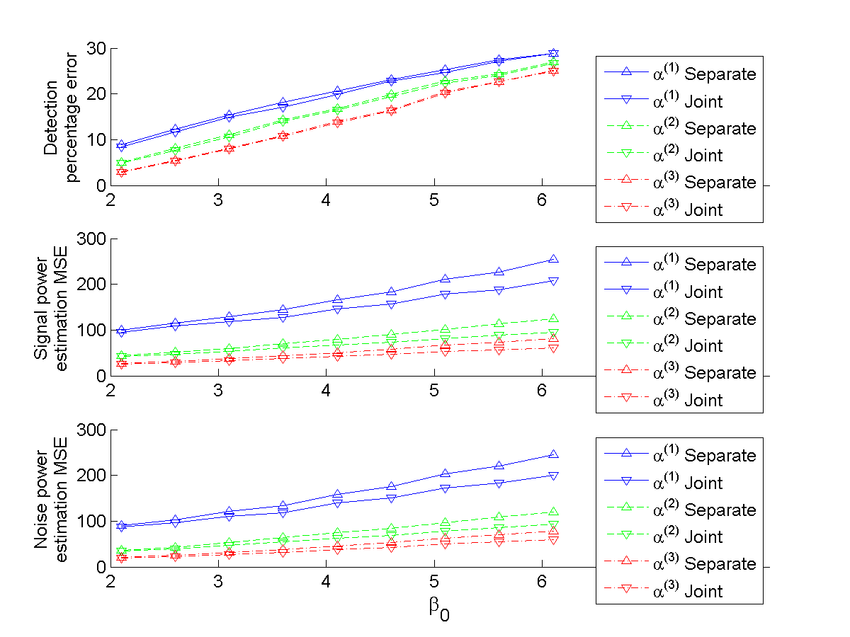
Figure 1: Performance comparison of detectors and estimators designed by the two approaches. In these simulations, the shape parameters are assumed to be the same $\alpha_{0}=\alpha_{1}=\alpha$, and the signal power scale is fixed $\beta_{1}=9.1$ while the noise power scale varies.

To demonstrate the utility of the derived detector and estimators, a set of simulations was carried out. For each simulation, 20,000 independent observation vectors, each of size 128, were randomly generated using a zero-mean Gaussian distribution with hypothesis-dependent power. The hypothesis $H_{1}$ and $H_{0}$ are equally likely and the power under $H_{0}$ and $H_{1}$ are generated using the inverse gamma distribution. The generic cost constants were set as follows $b_{00}=b_{11}=b_{01}=b_{10}=a_{01}=a_{10}=1$ and $a_{00}=a_{11}=0$ for simplicity. Finally, $\phi_{1}$ is set to 0 and $\phi_{2}$ to $\pi/8$ to impose the prior knowledge that signal power is usually much higher than noise power.

The proposed simultaneous approach was compared against the separate approach. The separate detection and estimation approach optimizes the detector and estimator separately. In summary, the detector’s test statistic is given by the generalized likelihood ratio

$$\Lambda=\frac{\langle f_{1}(\mathbf{y}|s,v)\rangle_{S,V}}{\langle f_{0}(\mathbf{y}|v)\rangle_{V}}\operatorname*{\gtrless}^{H_{1}}_{H_{0}}\frac{\pi_{0}}{\pi_{1}}$$

and the estimators are simply $\hat{s}^{H_{1}}$, $\hat{v}^{H_{1}}$, and $\hat{v}^{H_{0}}$.

Figure 1 shows that, for all three criteria, the optimal joint design approach outperforms the separate approach.

VI Conclusion

An optimal detector and signal and noise power estimators was jointly derived for the Gaussian observation model with appropriate conjugate priors on the signal and noise power. Future work will apply the developed techniques to improve widely used algorithms, such as Sohn’s VAD [6].

References

- [1] B. C. Levy, Principles of signal detection and parameter estimation. Springer, 2008.
- [2] D. Jones. (2004, May) Adaptive Equalization, Connexions. [Online]. Available: http://cnx.org/content/m11907/1.1/
- [3] Y. Wang and I. I. Hussein, “Bayesian-based decision-making for object search and classification,” Control Systems Technology, IEEE Transactions on, vol. 19, no. 6, pp. 1639–1647, 2011.
- [4] Y. Wang, I. Hussein, and R. Erwin, “Risk-based sensor management for integrated detection and estimation,” Journal of Guidance, Control, and Dynamics, vol. 34, no. 6, pp. 1767–1778, 2011.
- [5] L. Le, D. M. Jun, and D. L. Jones, “Energy efficient detection system in time varying signal and noise power,” in Acoustics, Speech and Signal Processing (ICASSP), 2013 IEEE International Conference on.
- [6] J. Sohn and W. Sung, “A voice activity detector employing soft decision based noise spectrum adaptation,” in Acoustics, Speech and Signal Processing, 1998. Proceedings of the 1998 IEEE International Conference on, vol. 1. IEEE, 1998, pp. 365–368.
- [7] J. Sohn, N. S. Kim, and W. Sung, “A statistical model-based voice activity detection,” Signal Processing Letters, IEEE, vol. 6, no. 1, pp. 1–3, 1999.
- [8] A. Abramson and I. Cohen, “Simultaneous detection and estimation approach for speech enhancement,” Audio, Speech, and Language Processing, IEEE Transactions on, vol. 15, no. 8, pp. 2348–2359, 2007.
- [9] Y. Ephraim and D. Malah, “Speech enhancement using a minimum-mean square error short-time spectral amplitude estimator,” Acoustics, Speech and Signal Processing, IEEE Transactions on, vol. 32, no. 6, pp. 1109–1121, 1984.
- [10] O. Cappé, “Elimination of the musical noise phenomenon with the Ephraim and Malah noise suppressor,” Speech and Audio Processing, IEEE Transactions on, vol. 2, no. 2, pp. 345–349, 1994.
- [11] D. Middleton and R. Esposito, “Simultaneous optimum detection and estimation of signals in noise,” Information Theory, IEEE Transactions on, vol. 14, no. 3, pp. 434–444, 1968.
- [12] A. Fredriksen, D. Middleton, and V. VandeLinde, “Simultaneous signal detection and estimation under multiple hypotheses,” Information Theory, IEEE Transactions on, vol. 18, no. 5, pp. 607–614, 1972.
- [13] G. V. Moustakides, “Optimum joint detection and estimation,” in Information Theory Proceedings (ISIT), 2011 IEEE International Symposium on. IEEE, 2011, pp. 2984–2988.
- [14] G. H. Jajamovich, A. Tajer, and X. Wang, “Optimal combined detection and estimation,” in Communication, Control, and Computing (Allerton), 2011 49th Annual Allerton Conference on. IEEE, 2011, pp. 1848–1852.
- [15] G. V. Moustakides, G. H. Jajamovich, A. Tajer, and X. Wang, “Joint detection and estimation: Optimum tests and applications,” Information Theory, IEEE Transactions on, vol. 58, no. 7, pp. 4215–4229, 2012.
- [16] J.-K. Hwang, “Simultaneous CFAR detection and frequency estimation of a sinusoidal signal in noise,” in Statistical Signal and Array Processing, 1992. Conference Proceedings., IEEE Sixth SP Workshop on. IEEE, 1992, pp. 78–81.
- [17] P. M. Djuric, “Simultaneous detection and frequency estimation of sinusoidal signals,” in Acoustics, Speech, and Signal Processing, 1993. ICASSP-93., 1993 IEEE International Conference on, vol. 4. IEEE, 1993, pp. 53–56.
- [18] B. Baygun and A. O. Hero III, “Optimal simultaneous detection and estimation under a false alarm constraint,” Information Theory, IEEE Transactions on, vol. 41, no. 3, pp. 688–703, 1995.
- [19] A. M. Sayeed and D. L. Jones, “Optimal detection using bilinear time-frequency and time-scale representations,” Signal Processing, IEEE Transactions on, vol. 43, no. 12, pp. 2872–2883, 1995.
- [20] I. Cohen and B. Berdugo, “Noise estimation by minima controlled recursive averaging for robust speech enhancement,” Signal Processing Letters, IEEE, vol. 9, no. 1, pp. 12–15, 2002.
- [21] I. Cohen, “Noise spectrum estimation in adverse environments: Improved minima controlled recursive averaging,” Speech and Audio Processing, IEEE Transactions on, vol. 11, no. 5, pp. 466–475, 2003.
- [22] T. Gerkmann and R. C. Hendriks, “Unbiased MMSE-based noise power estimation with low complexity and low tracking delay,” Audio, Speech, and Language Processing, IEEE Transactions on, vol. 20, no. 4, pp. 1383–1393, 2012.
- [23] R. Martin, “Noise power spectral density estimation based on optimal smoothing and minimum statistics,” Speech and Audio Processing, IEEE Transactions on, vol. 9, no. 5, pp. 504–512, 2001.
- [24] A. Gelman, J. B. Carlin, H. S. Stern, and D. B. Rubin, Bayesian data analysis. CRC press, 2003.
- [25] K. P. Murphy, “Conjugate Bayesian analysis of the Gaussian distribution,” def, vol. 1, no. 22, p. 16, 2007.