Transport gap and hysteretic behavior of the Ising quantum Hall ferromagnets in Landau levels $\left|N\right|>0$ of bilayer graphene

Abstract

The chiral two-dimensional electron gas in Landau levels $\left|N\right|>0$ of a Bernal-stacked graphene bilayer has a valley-pseudospin Ising quantum Hall ferromagnetic behavior at odd filling factors $\nu_{N}=1,3$ of these fourfold degenerate states. At zero interlayer electrical bias, the ground state at these fillings is spin polarized and electrons occupy one valley or the other while a finite electrical bias produces a series of valley pseudospin-flip transitions. In this work, we extend the Ising behavior to chirally-stacked multilayer graphene and discuss the hysteretic behavior of the Ising quantum Hall ferromagnets. We compute the transport gap due to different excitations: bulk electron-hole pairs, electron-hole pairs confined to the coherent region of a valley-pseudospin domain wall, and spin or valley-pseudospin skyrmion-antiskyrmion pairs. We determine which of these excitations has the lowest energy at a given value of the Zeeman coupling, bias, and magnetic field.

I INTRODUCTION

The chiral two-dimensional electron (C2DEG) gas in bilayer graphene (BLG) in a quantizing magnetic field exhibits a rich variety of broken-symmetry states in mean-field theory. These states have been extensively studiedbarlasreview in the zeroth-energy Landau level $N=0$ which is eightfold degenerate when valley $\left(K_{\pm}\right)$ and spin $\left(\sigma=\pm 1\right)$ degrees of freedom are counted because of the presence of an extra orbital degree of freedom $n=0,1$graphenereview . These broken symmetry states are best described using the pseudospin language where a valley pseudospin up(down) is associated with valley $K_{+}\left(K_{-}\right)$ and an orbital pseudospin up(down) is associated with the orbital $n=0(n=1).$ In this language, the broken-symmetry states are spin, valley, or orbital quantum Hall ferromagnets (QHFs). They are gapped, have charged quasiparticle excitations, and support an integer quantum Hall effectbarlasreview .

The effect of the Coulomb interaction on the higher Landau levels $\left|N\right|>0$ has so far received less attention. In a recent paperluo , we have shown that the C2DEG in these levels behaves as a valley Ising QHF when the filling factor of these levels (which are fourfold degenerate) is odd, i.e. when $\nu_{N}=1,3.$ The C2DEG at these fillings is spin polarized and the two valley states with valley pseudospin $P_{z}=\pm\frac{1}{2}$ are degenerate at zero and at some finite values of the bias $\Delta_{B}$ (the electrical potential difference between the two layers). For $\nu_{N}=2,$ transitions occur between states with total spin and total valley pseudospin $\left(S_{z},P_{z}\right)=\left(0,\pm 1\right),\left(1,0\right).$ Changing the bias can induce first-order transitions between the different spin and valley-pseudospin ground states. The phase diagram for different Landau levels shows a marked difference between the positive $N\geq 1$ and negative $N\leq-1$ Landau levels. The Ising behavior of the higher Landau levels contrasts with that of Landau level $N=0$ where valley, spin, or orbital QHF can all have a $U\left(1\right)$ symmetryjules .

Ising QHFs have been studied previously both theoreticallyquinn ; jungwirth ; jungwirth2 ; jungwirth3 and experimentallydaneshvar ; piazza in a variety of semiconductor quantum wells or bilayer systems. A complete classification of the QHF states, including isotropic, easy-axis, and easy-plane QHFs has been derived for a model of two nearby, infinitely narrow, two-dimensional layersjungwirthprb . A well-known case of Ising QHF occurs when two levels with different electrical subbands or Landau level indices are brought to degeneracy by tuning the electrical bias or the Zeeman coupling at even filling factor. The valley-pseudospin Ising transitions in the higher Landau levels, however, occur at odd filling factors and are of a slightly different nature: they do not occur near Landau level crossings. As in other Ising QHFs, however, the exchange part of the Coulomb interaction energy plays a major role as it competes with the noninteracting energy. What is special with BLG is that an electronic state is described by a four-component spinor and so consists of a superposition of four states with different orbital wave functions. As the bias is varied, the coefficients of this superposition are modified and so is the Coulomb exchange interaction which is orbital-dependent. In a way, the Ising transitions in BLG occur in part because of a change in the “internal structure” of the electron.

The discontinuous transitions between spin-polarized states at $\nu_{N}=2$ that occur when the bias is varied cause abrupt changes in the transport gap that may explain some recent experimental resultstutuc on the transport properties of the C2DEG in bilayer graphene. In the present work, we study the behavior of the transport gap of the C2DEG with bias at odd fillings of the higher Landau levels. We first show that the Ising behavior found previouslyluo should also occur in chirally-stacked multilayer graphene, at least at zero bias. We then compute the energy of different types of charged excitations of the Ising ground states. We consider bulk quasiparticles (quasi-electrons and quasi-holes) and topological quasiparticles (skyrmions and antiskyrmions). In each case, we evaluate the transport gap due to the excitation of a particle-antiparticle pair using a microscopic Hartree-Fock calculation. Our approach allows us to compute the excitation gap at finite Zeeman and/or bias and takes into account the possibility of intertwined spin and valley-pseudospin textures. When appropriate (at zero bias or Zeeman coupling), we also compute the transport gap using a long-wavelength approximation of the Hartree-Fock energy functional. When the Zeeman coupling is taken into account, we find that valley skyrmions are the lowest-energy excitations in bilayer graphene, at least for $N=\pm 1$. This contrasts with previously studied Ising systems where skyrmions are not the lowest-energy excitationslilliehook . The skyrmions that we find have either a spin or a valley-pseudospin texture, but not bothezawa ; gosh and, as in monolayer grapheneluo2 , they exist only in a small range of bias or Zeeman coupling.

Magnetic Ising ferromagnets show an hysteretic behavior of the magnetization as the magnetic field is swept upward or downward. In the absence of disorder and at $T=0,$ the external magnetic field must exceed a certain coercive field in order to produce the spin reversal. We find a similar behavior with bias for the valley pseudospins and so we compute the coercive bias for Landau levels $N=\pm 1.$ Owing to the fact that more valley-flip transitions are possible in levels $N>0$ than in $N<0,$ we find that the hysteretic behavior for $N>0$ is also more complex, with a very large coercive field.

At finite temperature or in a disordered system, domains with particular valley-pseudospin orientations are formed in the C2DEG. Regions of different valley pseudospins are separated by domain walls which can have complicated patterns. When domain walls are present, the electronic band structure and so the electron-hole excitation gap is modulated in space. In the coherent region of a domain wall, the valley pseudospins rotate from one polarization to the other. For a linear domain wall, the coherent region forms a linear channel of a few magnetic lengths in width. At the center of these regions, the band gap is minimal. It should be possible, then, to excite electron-holes pairs that are confined to a coherent region of a wall and that have smaller excitation energy than the bulk electron-hole or the skyrmion-antiskyrmion pairs. These mobile particles may be responsiblejungwirth for the increase in dissipation and breakdown of the quantum Hall effect that is observed in some Ising QHFspoortere . We compute the energy of such excitations and find that, in some range of bias, they can be the lowest-energy excitations.

This paper is organized in the following way. Sections II and III introduce the tight-binding model and the electronic states in bilayer graphene as well as most of the Hartree-Fock formalism necessary to derive the energy gap for the particle-antiparticle pairs. Section IV discusses the hysteretic behavior of the Ising QHFs and extend this behavior to other, chirally-stacked, multilayer graphene structures. The transport gaps for the electron-hole pairs, confined electron-hole pairs and skyrmion-antiskyrmion pairs are computed in Secs. V,VI, and VII respectively. Section VIII is the conclusion. The appendix provides a derivation of the projected representation of a skyrmion that is used in Sec. VII.

II TIGHT-BINDING MODEL

Bilayer graphene consists of two graphene layers separated by a distance $d=3.35$ Å. In each layer, the crystal structure is a honeycomb lattice that can be described as a triangular Bravais lattice with a basis of two carbon atoms $A_{m},B_{m}$ where $m=1,2$ is the layer index. The in-plane lattice constant is $a_{0}=2.46$ Å. In the Bernal stacking, the upper $A$ sublattice is directly on top of the lower $B$ sublattice, while the upper $B$ sublattice is above the center of a hexagonal plaquette of the lower layer. In the continuum approximation, the Hamiltonian is expanded around the two non-equivalent valley points $K_{\pm}=\pm\frac{4\pi}{3}\left(a_{0},0\right)$ of the Brillouin zonegraphenereview . In a transverse magnetic field $\mathbf{B}=B_{0}\widehat{\mathbf{z}}$, the tight-binding Hamiltonian for an electron with the valley index $\xi=\pm 1$ is given, in the basis $\left\{A_{1},B_{1},A_{2},B_{2}\right\},$ by

$$H_{\pm}^{\left(0\right)}=\left(\begin{array}[]{cccc}\delta_{0}+\frac{\Delta_{B}}{2}&\pm\alpha_{0}a^{\pm}&\pm\alpha_{4}a^{\mp}&-\gamma_{1}\\ \pm\alpha_{0}a^{\mp}&\frac{\Delta_{B}}{2}&0&\pm\alpha_{4}a^{\mp}\\ \pm\alpha_{4}a^{\pm}&0&-\frac{\Delta_{B}}{2}&\pm\alpha_{0}a^{\pm}\\ -\gamma_{1}&\pm\alpha_{4}a^{\pm}&\pm\alpha_{0}a^{\mp}&\delta_{0}-\frac{\Delta_{B}}{2}\end{array}\right),$$ (1)

where $\alpha_{i}=\sqrt{\frac{3}{2}}\frac{a_{0}}{\ell}\gamma_{i}$ with $\ell=\sqrt{\hslash c/eB}$ the magnetic length and $\gamma_{j}$ the hopping parameters. A recent calculationjung gives $\gamma_{0}=2.61$ eV for the nearest-neighbor hopping, $\gamma_{1}=-0.361$ eV for the interlayer hopping between carbon atoms that are immediately above one another (i.e. $A_{1}-B_{2}$) and $\gamma_{4}=-0.138$ eV for the interlayer next nearest-neighbor hopping between carbons atoms in the same sublattice (i.e. $A_{1}-A_{2}$ and $B_{1}-B_{2}$). The magnetic field considered in the present work is assumed sufficiently large for the warping term $\gamma_{3}$ to be negligiblemccann ; manuel . The parameter $\delta_{0}=0.015$ eV represents the difference in the crystal field between sites $A_{1},B_{2}$ and $A_{2},B_{1}$. The ladder operators $a^{-}=a$ and $a^{+}=a^{{\dagger}}$ are defined in the Landau gauge $\mathbf{A}=\left(0,Bx,0\right).$

In the absence of a magnetic field, the electronic dispersion has four bands which we denote by $j=1,2,3,4$ with $j=1,2$ the negative and $j=3,4$ the positive energy bands. The two middle bands $j=2,3$ touch each other at the six valley points $K_{\pm}$ where they have zero energy in the absence of bias. The high-energy bands $j=1,4$ are separated from the middle two energy bands by a gap of order $\gamma_{1}.$ In a quantizing magnetic field, each band is split into Landau levels. We shall be concerned only with bands $j=2,3$ in this work. The eigenstates of $H_{\pm}^{\left(0\right)}$ for the levels of these bands have energies $E_{\xi,n,j}^{\left(0\right)}$ with $n=0,1,2,...$ and the corresponding eigenvectors are given by

$$\psi_{\xi=-1,n,j,X}\left(\mathbf{r},z\right)=\left(\begin{array}[]{c}b_{\xi,n,j,1}h_{n-1,X}\left(\mathbf{r}\right)\chi_{1}\left(z\right)\\ b_{\xi,n,j,2}h_{n,X}\left(\mathbf{r}\right)\chi_{1}\left(z\right)\\ b_{\xi,n,j,3}h_{n-2,X}\left(\mathbf{r}\right)\chi_{2}\left(z\right)\\ b_{\xi,n,j,4}h_{n-1,X}\left(\mathbf{r}\right)\chi_{2}\left(z\right)\end{array}\right),$$ (2)

and

$$\psi_{\xi=+1,n,j,X}\left(\mathbf{r},z\right)=\left(\begin{array}[]{c}b_{\xi,n,j,1}h_{n-1,X}\left(\mathbf{r}\right)\chi_{1}\left(z\right)\\ b_{\xi,n,j,2}h_{n-2,X}\left(\mathbf{r}\right)\chi_{1}\left(z\right)\\ b_{\xi,n,j,3}h_{n,X}\left(\mathbf{r}\right)\chi_{2}\left(z\right)\\ b_{\xi,n,j,4}h_{n-1,X}\left(\mathbf{r}\right)\chi_{2}\left(z\right)\end{array}\right),$$ (3)

where $X$ is the guiding-center index. The functions $\left|\chi_{i}\left(z\right)\right|^{2}=\delta\left(z-z_{i}\right),$ where $z_{i}$ is the position of the graphene layer $i.$ By definition, $h_{n,X}\left(\mathbf{r}\right)=0$ if $n<0,$ otherwise

$$h_{n,X}\left(\mathbf{r}\right)=\frac{1}{\sqrt{L_{y}}}e^{-iXy/\ell^{2}}\varphi_{n}\left(x-X\right),$$ (4)

where $n$ is the level index and $L_{y}$ the sample dimension in the $y$ direction. The functions $\varphi_{n}\left(x\right)$ are the eigenstates of the one-dimensional harmonic oscillator.

In a minimal tight-binding model where only $\gamma_{0},\gamma_{1}$ are kept, levels $n=0,1$ are degenerate and have zero energy. When spin and valley degrees of freedom are counted and the Zeeman term is neglected, there are in total eight degenerate levels with zero energy. This octet of states defines the Landau level $N=0.$ The higher Landau levels have $n\geq 2$ with $j=2,3.$ The positive energy Landau levels $N=n-1$ have band index $j=3$ while the negative energy ones have $N=-\left(\left|n\right|-1\right)$ with $j=2.$ This notation is illustrated in Fig. 1 of Ref. luo, . Contrary to $N=0,$ the higher-energy Landau levels $\left|N\right|>0$ are fourfold degenerate. Each level with quantum numbers $\left(\xi,\sigma,n,j\right)$ has the macroscopic degeneracy $N_{\varphi}=S/2\pi\ell^{2},$ where $S$ is the C2DEG area, associated with the guiding-center index $X$.

In this work, we assume that Landau level mixing can be neglected. As shown in Ref. manuel, , this limits the electric bias to $\Delta_{B}$ $\lesssim 0.1$ eV for $B=10$ T and $\Delta_{B}$ $\lesssim 0.2$ eV for $B=30$ T. We project the Hamiltonian into level $N$ so that the electron field operator is given by

$$\Psi_{\mu,N}\left(\mathbf{r},z\right)=\sum_{X}\psi_{\mu,N,X}\left(\mathbf{r},z\right)c_{\mu,N,X},$$ (5)

where $c_{\mu,N,X}$ annihilates an electron is state $\left(\mu,N,X\right)$ and the super-index $\mu=\left(\xi,\sigma\right)$ corresponds to the four states

$$\mu = 1\rightarrow\left(K_{+},+\right),$$ (6)

$$\mu = 2\rightarrow\left(K_{+},-\right),$$ (7)

$$\mu = 3\rightarrow\left(K_{-},+\right),$$ (8)

$$\mu = 4\rightarrow\left(K_{-},-\right),$$ (9)

where the second index in the parenthesis is for the spin. Hereafter, we use the notation $\mu_{\xi}=\xi$ and $\mu_{\sigma}=\sigma.$

III HARTREE-FOCK FORMALISM FOR THE HIGHER LANDAU LEVELS

The various energy gaps are computed in this work in the Hartree-Fock approximation (HFA). In a recent work on the Ising QHFsluo , the HFA was used to compute the energy of ground states with uniform spin and/or valley polarizations. In this section, the HFA is extended to the study of excitations with spin and/or pseudospin textures. To simplify the notation, the subscript $N=\left(n,j\right)$ is omitted whenever possible, since the Hilbert space is restricted to level $N$ only.

III.1 Hartree-Fock Hamiltonian

The Hartree-Fock Hamiltonian for electrons in level $N$ is given by

$$\frac{H_{HF}}{N_{\varphi}} = -\alpha_{d}\frac{\nu_{N}^{2}}{4}+\frac{1}{2}\alpha_{d}\nu_{N}\left(\rho_{1}\left(0\right)+\rho_{2}\left(0\right)\right)$$

$$+\sum_{\mu}\left(E_{\mu_{\xi}}^{\left(0\right)}-\frac{1}{2}\mu_{\sigma}\Delta_{Z}\right)\rho_{\mu,\mu}\left(0\right)$$

$$-\alpha_{d}\left[\left\langle\rho_{1}\left(0\right)\right\rangle\rho_{2}\left(0\right)+\left\langle\rho_{2}\left(0\right)\right\rangle\rho_{1}\left(0\right)\right]$$

$$+\sum_{\mu,\mu^{\prime}}\overline{\sum_{\mathbf{q}}}H^{\left(\mu_{\xi},\mu_{\xi}^{\prime}\right)}\left(\mathbf{q}\right)\left\langle\rho_{\mu,\mu}\left(-\mathbf{q}\right)\right\rangle\rho_{\mu^{\prime},\mu^{\prime}}\left(\mathbf{q}\right)$$

$$-\sum_{\mu,\mu^{\prime}}\sum_{\mathbf{q}}X^{\left(\mu_{\xi},\mu_{\xi}^{\prime}\right)}\left(\mathbf{q}\right)\left\langle\rho_{\mu,\mu^{\prime}}\left(-\mathbf{q}\right)\right\rangle\rho_{\mu^{\prime},\mu}\left(\mathbf{q}\right),$$

where $\Delta_{Z}=g\mu_{B}B,$ with $g=2$ and $\mu_{B}$ the Bohr magneton, is the Zeeman coupling. The bar over the summation in the Hartree term means that the $\mathbf{q}=0$ is omitted from the sum because a positive background is considered in order to make the system neutral. We have defined the constant

$$\alpha_{d}=\frac{d}{\ell}\left(\frac{e^{2}}{\kappa\ell}\right)$$ (11)

and $\nu_{N}=N_{e}/N_{\varphi}$ is the filling factor of level $N$ with $N_{e}$ the number of electrons in this level. In $\alpha_{d},$ $\kappa$ is the dielectric constant of the substrate. In all the calculations of this paper, $\kappa=2.5.$

The ground state average value of the operators

$$\rho_{\mu,\mu^{\prime}}\left(\mathbf{q}\right) = \frac{1}{N_{\varphi}}\sum_{X,X^{\prime}}e^{-\frac{i}{2}q_{x}\left(X+X^{\prime}\right)}$$

$$\times\delta_{X,X^{\prime}+q_{y}\ell^{2}}c_{\mu,N}^{\dagger}c_{\mu^{\prime},X^{\prime}}$$

can be considered as the order parameters of a specific phase of the electron gas. The operators

$$\rho_{i}\left(0\right)=\sum_{\mu}n_{i,\mu_{\xi}}\rho_{\mu,\mu}\left(\mathbf{q}=0\right),$$ (13)

with $i=1,2$ and the projectors

$$n_{1,+} = \left|b_{4,+}\right|^{2}+\left|b_{3,+}\right|^{2},$$ (14)

$$n_{1,-} = \left|b_{1,-}\right|^{2}+\left|b_{2,-}\right|^{2},$$ (15)

$$n_{2,+} = \left|b_{1,+}\right|^{2}+\left|b_{2,+}\right|^{2},$$ (16)

$$n_{2,-} = \left|b_{3,-}\right|^{2}+\left|b_{4,-}\right|^{2},$$ (17)

and

$$n_{1} = n_{1,+}+n_{1,-},$$ (18)

$$n_{2} = n_{2,+}+n_{2,-},$$ (19)

are defined such that $\left\langle\rho_{i}\left(0\right)\right\rangle$ is the filling factor of layers $i=1,2$. It is important to remember that, unlike level $N=0,$ layer and valley indices are not equivalent in the higher Landau levels.

The Hartree and Fock interactions that enter $H_{HF}$ are defined by (here, $x=q\ell\,$)

$$H^{\left(\xi,\xi\right)}\left(x\right) = \left(\frac{e^{2}}{\kappa\ell}\right)\frac{V^{\left(\xi,\xi\right)}\left(x\right)}{x},$$ (20)

$$H^{\left(\xi,\overline{\xi}\right)}\left(x\right) = \left(\frac{e^{2}}{\kappa\ell}\right)\frac{V^{\left(\xi,\overline{\xi}\right)}\left(x\right)}{x},$$ (21)

$$X^{\left(\xi,\xi\right)}\left(x\right) = \left(\frac{e^{2}}{\kappa\ell}\right)\int_{0}^{\infty}dyV^{\left(\xi,\xi\right)}\left(y\right)J_{0}\left(xy\right),$$ (22)

$$X^{\left(\xi,\overline{\xi}\right)}\left(x\right) = \left(\frac{e^{2}}{\kappa\ell}\right)\int_{0}^{\infty}dyV^{\left(\xi,\overline{\xi}\right)}\left(y\right)J_{0}\left(xy\right),$$ (23)

with $\overline{\xi}=-\xi$ and ($G_{i}^{\left(\xi\right)}=G_{i}^{\left(\xi\right)}\left(x\right),$ for $i=1,2$) and

$$V^{\left(\xi,\xi\right)}\left(x\right) = G_{1}^{\left(\xi\right)}G_{1}^{\left(\xi\right)}+G_{2}^{\left(\xi\right)}G_{2}^{\left(\xi\right)}$$

$$+e^{-qd}\left[G_{1}^{\left(\xi\right)}G_{2}^{\left(\xi\right)}+G_{2}^{\left(\xi\right)}G_{1}^{\left(\xi\right)}\right],$$

$$V^{\left(\xi,\overline{\xi}\right)}\left(x\right) = G_{1}^{\left(\xi\right)}G_{2}^{\left(\overline{\xi}\right)}+G_{2}^{\left(\xi\right)}G_{1}^{\left(\overline{\xi}\right)}$$

$$+e^{-qd}\left[G_{1}^{\left(\xi\right)}G_{1}^{\left(\overline{\xi}\right)}+G_{2}^{\left(\xi\right)}G_{2}^{\left(\overline{\xi}\right)}\right],$$

with the functions

$$G_{1}^{\left(\xi\right)}\left(x\right) = e^{-x^{2}/4}\left[\left|b_{1,\xi}\right|^{2}L_{n-1}\left(\frac{x^{2}}{2}\right)\right.$$

$$\left.+\left|b_{2,\xi}\right|^{2}L_{n}\left(\frac{x^{2}}{2}\right)\right]$$

$$G_{2}^{\left(\xi\right)}\left(x\right) = e^{-x^{2}/4}\left[\left|b_{3,\xi}\right|^{2}L_{n-2}\left(\frac{x^{2}}{2}\right)\right.$$

$$+\left.\left|b_{4,\xi}\right|^{2}L_{n-1}\left(\frac{x^{2}}{2}\right)\right],$$

where $L_{n}\left(x\right)$ is a Laguerre polynomial.

The Hartree-Fock energy per electron is

$$\frac{E_{HF}}{N_{e}} = \frac{1}{\nu_{N}}\alpha_{d}\left[\left\langle\rho_{1}\left(0\right)\right\rangle-\left\langle\rho_{2}\left(0\right)\right\rangle\right]^{2}$$

$$+\frac{1}{\nu_{N}}\sum_{\mu}\left(E_{\mu_{\xi}}^{\left(0\right)}-\frac{\mu_{\sigma}\Delta_{Z}}{2}\right)\left\langle\rho_{\mu,\mu}\left(0\right)\right\rangle$$

$$+\frac{1}{2\nu_{N}}\sum_{\mu,\mu^{\prime}}\overline{\sum_{\mathbf{q}}}H^{\left(\xi,\zeta\right)}\left(\mathbf{q}\right)\left\langle\rho_{\mu,\mu}\left(-\mathbf{q}\right)\right\rangle\left\langle\rho_{\mu^{\prime},\mu^{\prime}}\left(\mathbf{q}\right)\right\rangle$$

$$-\frac{1}{2\nu_{N}}\sum_{\mu,\mu^{\prime}}\sum_{\mathbf{q}}X^{\left(\xi,\zeta\right)}\left(\mathbf{q}\right)\left\langle\rho_{\mu,\mu^{\prime}}\left(-\mathbf{q}\right)\right\rangle\left\langle\rho_{\mu^{\prime},\mu}\left(\mathbf{q}\right)\right\rangle.$$

III.2 Order parameters and single-particle Green’s functions

To compute the order parameters, we define the matrix of Matsubara Green’s functions

$$G_{\mu,\mu^{\prime}}\left(X,X^{\prime},\tau\right)=-\left\langle T_{\tau}c_{\mu,X}\left(\tau\right)c_{\mu^{\prime},X^{\prime}}^{\dagger}\left(0\right)\right\rangle,$$ (29)

where $T_{\tau}$ is the time-ordering operator. Its Fourier transform is defined by

$$G_{\mu,\mu^{\prime}}\left(\mathbf{q,}\tau\right) = \frac{1}{N_{\varphi}}\sum_{X,X^{\prime}}e^{-\frac{i}{2}q_{x}\left(X+X^{\prime}\right)}$$

$$\times\delta_{X,X^{\prime}-q_{y}\ell^{2}}G_{\mu,\mu^{\prime}}\left(X,X^{\prime},\tau\right),$$

so that

$$\left\langle\rho_{\mu^{\prime},\mu}\left(\mathbf{q}\right)\right\rangle=G_{\mu,\mu^{\prime}}\left(\mathbf{q,}\tau=0^{-}\right).$$ (31)

The matrix of Green’s functions is computed from its Hartree-Fock equation of motion

$$\left[\hslash i\omega_{n}-\left(E_{\mu}-\widetilde{\mu}\right)\right]G_{\mu,\mu^{\prime}}\left(\mathbf{q},\omega_{n}\right)=\hslash\delta_{\mathbf{q},0}\delta_{\mu,\mu^{\prime}}$$ (32)

$$+\sum_{\mu^{\prime\prime}}\overline{\sum_{\mathbf{q}^{\prime}\neq\mathbf{q}}}H^{\left(\mu_{\xi}^{\prime\prime},\mu_{\xi}\right)}\left(\mathbf{q}^{\prime}-\mathbf{q}\right)\left\langle\rho_{\mu^{\prime\prime},\mu^{\prime\prime}}\left(\mathbf{q-q}^{\prime}\right)\right\rangle$$

$$\times e^{-i\left(\mathbf{q}\times\mathbf{q}^{\prime}\right)\cdot\widehat{\mathbf{z}}\ell^{2}/2}G_{\mu,\mu^{\prime}}\left(\mathbf{q}^{\prime},\omega_{n}\right)$$

$$-\sum_{\mu^{\prime\prime}}\sum_{\mathbf{q}^{\prime}}X^{\left(\mu_{\xi}^{\prime\prime},\mu_{\xi}\right)}\left(\mathbf{q}^{\prime}-\mathbf{q}\right)\left\langle\rho_{\mu^{\prime\prime},\mu}\left(\mathbf{q-q}^{\prime}\right)\right\rangle$$

$$\times e^{-i\left(\mathbf{q}\times\mathbf{q}^{\prime}\right)\cdot\widehat{\mathbf{z}}\ell^{2}/2}G_{\mu^{\prime\prime},\mu^{\prime}}\left(\mathbf{q}^{\prime},\omega_{n}\right),$$

where $\widetilde{\mu}$ is the chemical potential and the renormalized energies are given by

$$E_{\mu}=E_{\mu_{\xi}}^{\left(0\right)}-\frac{1}{2}\mu_{\sigma}\Delta_{Z}+\sum_{\mu^{\prime}}A^{\left(\mu_{\xi},\mu_{\xi}^{\prime}\right)}\left\langle\rho_{\mu^{\prime},\mu^{\prime}}\left(0\right)\right\rangle,$$ (33)

where

$$A^{\left(\pm,\pm\right)} = -2\alpha_{d}n_{2,\pm}n_{1,\pm},$$ (34)

$$A^{\left(\pm,\mp\right)} = -\alpha_{d}\left(n_{2,+}n_{1,-}+n_{1,+}n_{2,-}\right).$$ (35)

III.3 Hartree-Fock energy in the pseudospin language

It is instructive to rewrite the Hartree-Fock energy in a pseudospin language. Since the skyrmions found in the HFA do not contain intertwined spin and valley-pseudospin textures, it is sufficient to define pure spin and valley-pseudospin fields. For the total spin field, including both valleys,

$$S_{z} = \frac{1}{2}\sum_{\mu}\mu_{\sigma}\left\langle\rho_{\mu,\mu}\right\rangle,$$ (36)

$$S_{x}+iS_{y} = \left\langle\rho_{1,2}\right\rangle+\left\langle\rho_{3,4}\right\rangle.$$ (37)

For the total valley pseudospin, including both spin states,

$$P_{z} = \frac{1}{2}\sum_{\mu}\mu_{\xi}\left\langle\rho_{\mu,\mu}\right\rangle,$$ (38)

$$P_{x}+iP_{y} = \left\langle\rho_{1,3}\right\rangle+\left\langle\rho_{2,4}\right\rangle.$$ (39)

Finally, for the total electronic density

$$\rho=\sum_{\mu}\left\langle\rho_{\mu,\mu}\right\rangle.$$ (40)

The Fourier transform of these fields is defined by

$$\mathbf{F}\left(\mathbf{r}\right)=\frac{1}{S}\sum_{\mathbf{q}}e^{i\mathbf{q}\cdot\mathbf{r}}\mathbf{f}\left(\mathbf{q}\right),$$ (41)

where $\mathbf{F}\left(\mathbf{r}\right)$ is one of the fields and $\mathbf{f}\left(\mathbf{q}\right)$ is defined in term of the order parameters $\left\{\left\langle\rho_{\mu,\mu^{\prime}}\left(\mathbf{q}\right)\right\rangle\right\}.$ It does not include the form factors that reflect the character of the different orbitals present in the electronic spinor (see Eqs. (2) and (3)). We say that $\mathbf{F}\left(\mathbf{r}\right)$ is given in the guiding-center representation (GCR).

We define the field $\mathbf{S}_{\xi}$ as the part of the total spin field which is in valley $\xi$ while $\mathbf{P}_{\bot,\sigma}$ is the part of the total in-plane valley-pseudospin field with spin $\sigma$. The fields are coupled by the constraint

$$\sum_{\mathbf{q}}\left[\frac{1}{4}\left|\rho\right|^{2}+\left|P_{z}\right|^{2}+2\left|P_{\bot,+}\right|^{2}+2\left|P_{\bot,-}\right|^{2}\right.$$

$$\left.+2\left|\mathbf{S}_{+}\right|^{2}+2\left|\mathbf{S}_{-}\right|^{2}+2\left|\left\langle\rho_{1,4}\right\rangle\right|^{2}+2\left|\left\langle\rho_{2,3}\right\rangle\right|^{2}\right]$$

$$= \nu_{N},$$

where $\rho=\rho\left(\mathbf{q}\right),P_{z}=P_{z}\left(\mathbf{q}\right),$ etc.

In the GCR, the Hartree-Fock energy per electron $E_{HF}$ becomes

$$\frac{E_{HF}}{N_{e}} = \frac{1}{\nu_{N}}\sum_{\xi}\left(\frac{\rho\left(0\right)}{2}E_{\mu_{\xi}}^{\left(0\right)}+\xi E_{\mu_{\xi}}^{\left(0\right)}P_{z}\left(0\right)\right)$$

$$+\frac{1}{4\nu_{N}}\alpha_{d}\left(\left\langle\rho_{1}\left(0\right)\right\rangle-\left\langle\rho_{2}\left(0\right)\right\rangle\right)^{2}-\Delta_{Z}S_{z}\left(0\right)$$

$$+\frac{1}{8\nu_{N}}\sum_{\mathbf{q}}\Lambda_{\rho,\rho}\left(\mathbf{q}\right)\left|\rho\left(\mathbf{q}\right)\right|^{2}$$

$$+\frac{1}{2\nu_{N}}\sum_{\mathbf{q}}\Lambda_{z,z}\left(\mathbf{q}\right)\left|P_{z}\left(\mathbf{q}\right)\right|^{2}$$

$$+\frac{1}{2\nu_{N}}\sum_{\mathbf{q}}\Lambda_{\rho,z}\left(\mathbf{q}\right)\rho\left(-\mathbf{q}\right)P_{z}\left(\mathbf{q}\right)$$

$$-\frac{1}{\nu_{N}}\sum_{\mathbf{q}}\sum_{\xi}X^{\left(\xi,\xi\right)}\left(\mathbf{q}\right)\left|\mathbf{S}_{\xi}\left(\mathbf{q}\right)\right|^{2}$$

$$-\frac{1}{\nu_{N}}\sum_{\mathbf{q}}\sum_{\sigma}X^{\left(+,-\right)}\left(\mathbf{q}\right)\left|\mathbf{P}_{\bot,\sigma}\left(\mathbf{q}\right)\right|^{2}$$

$$-\frac{1}{2\nu_{N}}\sum_{\mathbf{q}}X^{\left(+,-\right)}\left(\mathbf{q}\right)\left|\left\langle\rho_{1,4}\left(\mathbf{q}\right)\right\rangle\right|^{2}$$

$$-\frac{1}{2\nu_{N}}\sum_{\mathbf{q}}X^{\left(+,-\right)}\left(\mathbf{q}\right)\left|\left\langle\rho_{2,3}\left(\mathbf{q}\right)\right\rangle\right|^{2}.$$

The interactions are functions of $x=\left|\mathbf{q\ell}\right|$ only and are given by

$$\Lambda_{\rho,\rho} = \sum_{\xi}\left[H^{\left(\xi,\xi\right)}+H^{\left(\xi,\overline{\xi}\right)}-\frac{1}{2}X^{\left(\xi,\xi\right)}\right],$$ (44)

$$\Lambda_{\rho,z} = \sum_{\xi}\xi\left[H^{\left(\xi,\xi\right)}-\frac{1}{2}X^{\left(\xi,\xi\right)}\right],$$ (45)

$$\Lambda_{z,z} = \sum_{\xi}\left[H^{\left(\xi,\xi\right)}-H^{\left(\xi,\overline{\xi}\right)}-\frac{1}{2}X^{\left(\xi,\xi\right)}\right].$$ (46)

III.4 Gradient approximation of the Hartree-Fock energy

In the limit of zero Zeeman or bias coupling, skyrmions usually become very large and their energies cannot be computed by the microscopic HFA of Eq. (32) since the matrix of Green’s functions becomes very large. In this limit, it is more useful to make a gradient approximation of the total energy in Eq. (III.3), taking advantage of the fact that the spin or pseudospin texture varies slowly in spacemoon so that only the first few terms in the expansion can be kept. In levels $\left|N\right|>0$ of bilayer graphene, the gradient approximation works well for spin skyrmion but, as we will show below, cannot be applied to valley-pseudospin skyrmions since these later topological excitations have a small finite size at zero bias.

III.4.1 Spin textures

When all electrons occupy the valley $K_{\xi}$ at $\nu_{N}=1$, there is no intervalley coherence and Eq. (III.3) at zero bias and zero Zeeman coupling simplifies to

$$E_{\mathrm{spin}} = N_{\varphi}E_{\xi}^{\left(0\right)}+\frac{1}{4}N_{\varphi}\alpha_{d}\left(n_{1,\xi}-n_{2,\xi}\right)^{2}$$

$$+\frac{1}{2}N_{\varphi}\sum_{\mathbf{q}}\widetilde{\Lambda}_{\rho,\rho}^{\left(\xi\right)}\left(\mathbf{q}\right)\left|\rho\left(\mathbf{q}\right)\right|^{2}$$

$$-N_{\varphi}\sum_{\mathbf{q}}X^{\left(\xi,\xi\right)}\left(\mathbf{q}\right)\left|\mathbf{S}_{\xi}\left(\mathbf{q}\right)\right|^{2},$$

with

$$\widetilde{\Lambda}_{\rho,\rho}^{\left(\xi\right)}=H^{\left(\xi,\xi\right)}-\frac{1}{2}X^{\left(\xi,\xi\right)}.$$ (48)

Note that, at zero bias,

$$n_{1,\pm} = n_{2,\mp},$$ (49)

$$E_{+}^{\left(0\right)} = E_{-}^{\left(0\right)}\equiv E^{\left(0\right)},$$ (50)

$$H^{\left(+,+\right)} = H^{\left(-,-\right)}\equiv H,$$ (51)

$$X^{\left(+,+\right)} = X^{\left(-,-\right)}\equiv X,$$ (52)

$$V^{\left(+,+\right)} = V^{\left(-,-\right)}\equiv V,$$ (53)

so that $E_{\mathrm{spin}}$ is independent of the valley index.

For a spin-textured excitation, all electrons remain in the same valley but some of them flip their spin. If we neglect the charge density term (i.e. the third term on the right-hand side of Eq. (III.4.1)), then a gradient approximation gives for the excitation energy with respect to the ground state

$$\delta E_{\mathrm{spin}}=\frac{1}{2}\rho_{S}\sum_{\nu}\int d\mathbf{r}\left(\partial_{\nu}\mathbf{s}_{\xi}\left(\mathbf{r}\right)\right)^{2},$$ (54)

where $\nu=x,y$ and the field $\mathbf{s}_{\xi}\left(\mathbf{r}\right)\equiv 2S\mathbf{S}_{\xi}\left(\mathbf{r}\right)$ (where $S$ is the 2DEG area) has unit modulusnote4 . The spin stiffness is defined by

$$\rho_{S}=\frac{1}{16\pi}\left(\frac{e^{2}}{\kappa\ell}\right)\int_{0}^{\infty}dyV\left(y\right)y^{2}.$$ (55)

Eq. (54), with the condition that $\left|\mathbf{s}_{\xi}\left(\mathbf{r}\right)\right|=1,$ is the nonlinear $\sigma$ model (NL$\sigma$M). Note that, $\delta E_{\mathrm{spin}}$ is the energy of an uncharged spin texture. No electron is added or removed to the system. To compute the energy of a charged spin texture, it is necessary to consider the chemical potentialmoon . There is no need to worry about this problem in the present work since we are interested only in the transport gap which is the energy required to excite a skyrmion-antiskyrmion pair. This energy can be expressed solelygirvin in terms of $\rho_{S}$ (see Eq. (118) below).

A finite Zeeman coupling favors small spin textures while the charge-density term favors large textures. At finite Zeeman coupling, the size of the spin texture is a compromise between these two terms and it can be small. The gradient approximation is then no longer valid. A microscopic Hartree-Fock calculation must be done to compute the energy of small spin textures.

III.4.2 Valley-pseudospin textures

When all electrons occupy the spin state $\sigma=+1$ at $\nu_{N}=1$, there is no spin coherence and the total Hartree-Fock energy at zero bias is

$$E_{\mathrm{valley}} = N_{\varphi}\left(E^{\left(0\right)}-\frac{\Delta_{B}}{2}\right)$$

$$+\frac{1}{16}N_{\varphi}\alpha_{d}\left(n_{1}-n_{2}\right)^{2}$$

$$+N_{\varphi}\alpha_{d}\left(n_{1,+}-n_{1,-}\right)^{2}P_{z}^{2}(0)$$

$$+\frac{1}{4}N_{\varphi}\sum_{\mathbf{q}}\Upsilon_{\rho,\rho}\left(\mathbf{q}\right)\left|\rho\left(\mathbf{q}\right)\right|^{2}$$

$$+N_{\varphi}\sum_{\mathbf{q}}\Upsilon_{z,z}\left(\mathbf{q}\right)\left|P_{z,+}\left(\mathbf{q}\right)\right|^{2}$$

$$-N_{\varphi}\sum_{\mathbf{q}}X^{\left(+,-\right)}\left(\mathbf{q}\right)\left|\mathbf{P}_{\bot,+}\left(\mathbf{q}\right)\right|^{2},$$

where

$$\Upsilon_{\rho,\rho} = H-X+H^{\left(+,-\right)},$$ (57)

$$\Upsilon_{z,z} = H-X-H^{\left(+,-\right)}.$$ (58)

In a valley-pseudospin texture, no spin are flipped. Neglecting again the charge-density term, the gradient approximation gives for the excitation energy with respect to an Ising ground state with $P_{z}\left(0\right)=\xi/2$

$$\delta E_{\mathrm{valley}} = K\int d\mathbf{r}\left[p_{z}^{2}\left(\mathbf{r}\right)-1\right]$$

$$+\frac{1}{2}\sum_{\nu}\int d\mathbf{r}\left[\rho_{z}\left(\partial_{\nu}p_{z}\left(\mathbf{r}\right)\right)^{2}+\rho_{\bot}\left(\partial_{\nu}p_{\bot}\left(\mathbf{r}\right)\right)^{2}\right]$$

$$+N_{\varphi}\alpha_{d}\left(n_{1,+}-n_{1,-}\right)^{2}\left[\left(P_{z}(q=0)\right)^{2}-\frac{1}{4}\right],$$

where $\mathbf{p}\left(\mathbf{r}\right)=2S\mathbf{P}\left(\mathbf{r}\right)$ is a unit field and the pseudospin stiffnesses are given by

$$\rho_{\bot}=\frac{1}{16\pi}\left(\frac{e^{2}}{\kappa\ell}\right)\int_{0}^{\infty}dyV^{\left(+,-\right)}\left(y\right)y^{2},$$ (60)

and

$$\rho_{z}=\rho_{S}=\frac{1}{16\pi}\left(\frac{e^{2}}{\kappa\ell}\right)\int_{0}^{\infty}dyV\left(y\right)y^{2},$$ (61)

while the easy-axis anisotropy term is given by

$$K=-\frac{1}{8\pi\ell^{2}}\left(X\left(0\right)-X^{+,-}\left(0\right)\right).$$ (62)

The last term in Eq. (III.4.2) is related to the capacitive energy. If $N_{\overline{\xi}}<<N_{\varphi},$ it can be rewritten as

$$-\alpha_{d}\left(n_{1,R}-n_{1,L}\right)^{2}\frac{N_{\xi}N_{\overline{\xi}}}{N_{\varphi}}\approx-\alpha_{d}\left(n_{1,R}-n_{1,L}\right)^{2}N_{\overline{\xi}},$$ (63)

where $N_{\xi}$ is the number of electrons in valley $\xi.$ Even though the bias is zero, there is a capacitive energy because in each state $K_{\xi},$ there is a charge imbalance between the two layers which is given by

$$\rho_{1}\left(0\right)-\rho_{2}\left(0\right)=\xi\left(n_{1,+}-n_{2,+}\right).$$ (64)

Numerically, $\rho_{S},\rho_{\bot}$ and $K$ are all positive quantities. As an example, for $N=-1,B=10$ T, their value is $\rho_{z}=0.97$ meV$,\rho_{\bot}=0.85$ meV, $K=-0.048$ meV/$\ell^{2}$ and $\alpha_{d}\left(n_{1,+}-n_{1,-}\right)^{2}=0.029$ meV. The easy-axis anisotropy and capacitive energy are comparable in size.

IV QUANTUM HALL ISING FERROMAGNETS

In this section, we extend the Ising behavior of bilayer grapheneluo to chirally-stacked multilayer graphene and discuss the hysteretic behavior associated with the valley-pseudospin flip transitions at integer filling $\nu_{N}=1.$

IV.1 Valley Ising quantum ferromagnetism and hysteretic behavior

The ground state at $\nu_{N}=1$ is spin polarized and so, for a uniform state, the energy functional of Eq. (III.3) simplifies to (with $P_{z}\left(\mathbf{q}=0\right)=\frac{1}{2}\cos\theta$)

$$e_{HF}\left(\theta\right)=\frac{E_{HF}\left(\theta\right)}{N_{e}}=C+\alpha\cos\left(\theta\right)+\beta\cos^{2}\left(\theta\right),$$ (65)

where $C$ is a constant and $\alpha,\beta,$ which depend implicitly on the bias $\Delta_{B},$ are given by

$$\alpha=\frac{1}{2}\sum_{\xi}\left(\xi E_{\xi}^{\left(0\right)}-\frac{1}{2}\xi X^{\left(\xi,\xi\right)}-\xi\alpha_{d}n_{1,\xi}n_{2,\xi}\right)$$ (66)

and

$$\beta = \frac{\alpha_{d}}{4}\left(n_{1,+}-n_{1,-}\right)^{2}$$

$$-\frac{1}{8}\left(X^{\left(+,+\right)}+X^{\left(-,-\right)}-2X^{\left(+,-\right)}\right)$$

with all interactions evaluated at $\mathbf{q}=0.$ The form of the energy functional $e_{HF}\left(\theta\right)$ (with $C$ neglected) is shown in Fig. 1(a) for a finite bias. There are two extrema at $\theta=0$ and $\theta=\pi$ and another one at $\cos\left(\theta^{\ast}\right)=-\alpha/2\beta$ with respective energies

$$E_{\theta=0} = \alpha+\beta,$$ (68)

$$E_{\theta=\pi} = -\alpha+\beta,$$ (69)

$$E_{\theta^{\ast}} = -\alpha^{2}/4\beta.$$ (70)

The metastable minimum (chosen to be $\theta=\pi$ in the figure) disappears when the curvature of $e_{HF}\left(\theta\right)$ changes sign or, equivalently, when $E_{\theta=0}=E_{\theta^{\ast}}$ or $E_{\theta=\pi}=E_{\theta^{\ast}}.$ We show in Fig. 1(b) and (c) the behavior of these three energies for $N=-1$ at $B=10$ T and $N=1$ at $B=21$ T.

When $\alpha=0$ and $\beta<0,$ or equivalently,

$$X^{\left(+,+\right)}-X^{\left(+,-\right)}>\alpha_{d}\left(n_{1,+}-n_{1,-}\right)^{2},$$ (71)

the two states $P_{z}\left(0\right)=\pm\frac{1}{2}$ are degenerate and the C2DEG has an Ising behavior. This situation occurs at zero bias.

Numerically, the coefficient $\beta<0$ at all bias but $\alpha\neq 0$. As Fig. 1 shows, $E_{\theta=0},E_{\theta=\pi}<E_{\theta^{\ast}}$ so that the Ising behavior persists to finite bias although the two minima at $\theta=0,\pi$ then have unequal energies. One minimum is a metastable state and the other a stable state. A hysteretic behavior is expected since the system can be trapped into the metastable state if the thermal energy is not sufficient to overcome the energy barrier between the two minima. A similar behavior was discussed in semiconductor Ising QHFsjungwirthprb , but the hysteretic behavior found in bilayer graphene for valley pseudospins seems more complex.

For $N=-1,$ the coefficient $\alpha=0$ only at zero bias where there is a transition from $P_{z}=\frac{1}{2}$ ($\Delta_{B}<0$) to $P_{z}=-\frac{1}{2}$ ($\Delta_{B}>0$). In the ground state, all electrons are in the valley which has the lowest non-interacting energy $E_{\xi}^{\left(0\right)}$. This is the situation depicted in Fig. 1(b). For positive bias, the metastable state at $\theta=0$ disappears at the bias $\Delta_{B}^{\left(\mathrm{coer}\right)}=4.2$ meV where $E_{\theta=0}=E_{\theta^{\ast}}$. In analogy with a magnetic system, $\Delta_{B}^{\left(\mathrm{coer}\right)}$ can be considered as a coercive bias. For negative bias, $\theta=\pi$ is the metastable state and a similar scenario occurs. Hereafter, we consider positive bias only since the transitions for negative bias are the opposite of those for positive bias. All Landau levels $N<-1$ behave in the same fashion. The smallness of $\Delta_{B}^{\left(\mathrm{coer}\right)}$ for $N=-1$ reflects the fact that $\alpha$ increases very rapidly with bias.

For $N=1,$ the ground state has $P_{z}=\frac{1}{2}$ at finite bias (the electrons are in the valley state with the biggest non-interacting energy) until a critical bias $\Delta_{B}^{\left(c\right)}=152$ meV indicated in Fig. 1(c) where there is a jump from $P_{z}=+\frac{1}{2}$ to $P_{z}=-\frac{1}{2}$. Unlike $N=-1,$ the two minima in $e_{HF}\left(\theta\right)$ coexist up to a very large coercive bias $\Delta_{B}^{\left(\mathrm{coer}\right)}=808$ meV that is well outside the limit of validity of our model that assumes no Landau level mixing. In order to find the correct coercive bias for $N=1,$ it is necessary to include this mixing.

We discuss the hysteretic loop for $N=\pm 1$ below (see Fig. 3 (c)), after we obtain the gap for the bulk and confined electron-hole excitations.

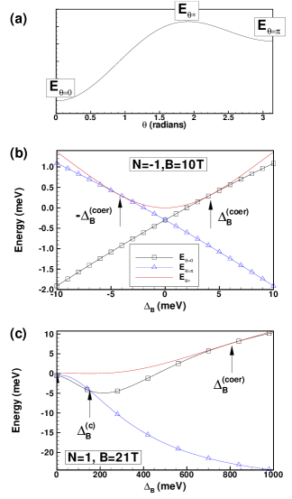
Figure 1: (Color online) (a) General form of the energy functional $e_{HF}\left(\theta\right)$ with the two minima at $\theta=0,\pi$ and the maximum at $\theta^{\ast}.$ Energy per electron at the extremal values of $e_{HF}\left(\theta\right)$ for (b) $N=-1,B=10T;$ (c) $N=1,B=21$ T.

IV.2 Ising behavior in multilayer graphene

The Ising behavior can be extended to chirally-stacked $m-$layer graphene ($m>1$), at least at zero bias. In the simplest tight-binding model where only $\gamma_{0}$ and $\gamma_{1}$ are kept and in the two-component modelmccann , the Hamiltonian in the basis $\left(A_{1},B_{m}\right)$ is

$$H_{\xi}=a^{m-1}\alpha_{0}\xi^{m}\left(\begin{array}[]{cc}0&\left(a^{\xi}\right)^{m}\\ \left(a^{-\xi}\right)^{m}&0\end{array}\right),$$ (72)

where $a=\alpha_{0}/\gamma_{1}.$ The eigenvectors are of the form

$$\frac{1}{\sqrt{2}}\left(\begin{array}[]{c}h_{n}\left(\mathbf{r}\right)\\ c_{m}h_{n-m}\left(\mathbf{r}\right)\end{array}\right),$$ (73)

with $\left|c_{m}\right|^{2}=1.$ (Landau level $\left|N\right|=1$ corresponds to $n=m.$) This model can be captured by our approach if only two-coefficients in the spinors of Eqs. (2,3) are kept. This implies, from Eqs. (14-17), that $n_{1,\pm}=n_{2,\mp}=1/2.$ The Ising criteria in Eq. (71), becomes

$$X^{\left(+,+\right)}-X^{\left(+,-\right)}>0$$ (74)

or

$$\int_{0}^{\infty}dye^{\frac{-y^{2}}{2}}A^{2}\left(y\right)\left(1-e^{-\left(m-1\right)yd/\ell}\right)>0,$$ (75)

with

$$A\left(y\right)=L_{n}^{0}\left(\frac{y^{2}}{2}\right)-L_{n-m}^{0}\left(\frac{y^{2}}{2}\right),$$ (76)

where $d$ is the separation between two adjacent layers. This inequality is satisfied for $m>1$ in chirally-stacked multilayer graphene.

V EXCITATION GAP FOR BULK ELECTRON-HOLE PAIRS

We now study the charged excitations of the Ising QHFs at $\nu_{N}=1$ in Landau levels $N=\pm 1.$ We start in this section with the Hartree-Fock bulk quasiparticles (electron and hole) and consider in the next two sections the Hartree-Fock electron and hole quasiparticles confined to the coherent region of a valley-pseudospin domain wall and the spin and/or valley-pseudospin skyrmions and antiskyrmions. In each case, we are mostly interested in computing the energy to create a quasiparticle-antiquasiparticle pair with infinite separation which is simply the sum of the quasiparticle and antiquasiparticle energies. The minimal such energy defines the transport gap of the Ising QHF which is measurable in transport experiment.

In the uniform Ising phases, the equation of motion for the matrix of Green’s functions (Eq. (32)) gives four energy levels. When the ground state is $\mu=1$ (i.e. $\mu_{\xi}=1$), the only nonzero order parameter is $\left\langle\rho_{1,1}\left(0\right)\right\rangle=1$ while when $\mu=3$ (i.e. $\mu_{\xi}=-1$) the only parameter is $\left\langle\rho_{3,3}\left(0\right)\right\rangle=1.$ The first energy level is fully occupied and amongst the three possible bulk electron-hole excitations, two are always lower in energy: a spin flip and a valley-pseudospin flip. For a ground state in valley $\xi,$ the spin and valley flips have the energy

$$\Delta_{\mathrm{spin},\xi} = \Delta_{Z}+X_{N}^{\left(\xi,\xi\right)},$$ (77)

$$\Delta_{\mathrm{valley},\xi} = E_{-\xi}^{\left(0\right)}-E_{\xi}^{\left(0\right)}$$

$$+A_{N}^{\left(\xi,-\xi\right)}-A_{N}^{\left(\xi,\xi\right)}+X_{N}^{\left(\xi,\xi\right)}.$$

These energies are plotted as a function of the bias in Fig. 2(a) for $N=-1,B=10$ T and Fig. 2(b) for $N=1,B=21$T. For $N=-1,$ the lowest-energy bulk excitation (i.e. the transport gap) is a valley-pseudospin flip at small bias and it changes to a spin flip above $\Delta_{B}^{(\ast)}=12.2$ meV. There is a discontinuity in the slope of the gap at $\Delta_{B}^{(\ast)}.$ For $N=1,$ the lowest-energy excitation is also a valley-pseudospin flip until the critical bias $\Delta_{B}^{\left(c\right)}=152$ meV. At this bias, a ground state transition causes a discontinuity in the gap: it abruptly changes from a valley-pseudospin flip to a spin flip. This is indicated by a the downward arrow in Fig. 2.

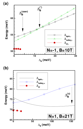
Figure 2: (Color online) Energy of the bulk ($\Delta_{\mathrm{spin},\xi}$ and $\Delta_{\mathrm{valley},\xi}$) and confined ($\Delta_{\mathrm{cf},-}$) electron-hole excitations as a function of bias for: (a) $N=-1,B=10$ T and (b) $N=1,B=21$ T.

VI EXCITATION GAP FOR ELECTRON-HOLE PAIRS CONFINED TO DOMAIN WALLS

In the presence of disorder or at finite temperature, domain walls (DW) are created in an Ising ferromagnetjungwirth . These walls can have different shapes, even closing on themselves (i.e. domain wall loops). In this section, we find a straight domain wall solution to the microscopic Hartree-Fock equation and compute the minimal energy required to excite an electron-hole pair in its coherent region.

At filling factor $\nu_{N}=1,$ the ground state is spin polarized and all electrons must be in valley $\xi=+1$ or $\xi=-1.$ For a state modulated in only one direction, say along $x$, we can take $q_{y}=0$ in the definition of the Fourier transform of the Green’s function in Eq. (III.2) and so

$$G_{\xi,\xi^{\prime}}\left(X,\tau\right)=-\left\langle Tc_{\xi,X}\left(\tau\right)c_{\xi^{\prime},X}^{\dagger}\left(0\right)\right\rangle.$$ (79)

The order parameters are now given by

$$\left\langle\rho_{\xi,\xi^{\prime}}\left(X\right)\right\rangle = \left\langle c_{\xi^{\prime},X}^{{\dagger}}c_{\xi,X}\right\rangle$$

$$= G_{\xi^{\prime},\xi}\left(X,\tau=0^{-}\right).$$

The equation of motion (Eq. (32)) simplifies to

$$\left[\hslash i\omega_{n}-\left(\widetilde{E}_{\xi}-\widetilde{\mu}\right)\right]G_{\xi,\xi^{\prime}}\left(X,\omega_{n}\right)=\hslash\delta_{\xi,\xi^{\prime}}$$ (81)

$$+H^{\xi}\left(X\right)G_{\xi,\xi^{\prime}}\left(X,\omega_{n}\right)-\sum_{\xi^{\prime\prime}}X^{\xi,\xi^{\prime\prime}}\left(X\right)G_{\xi^{\prime\prime},\xi^{\prime}}\left(X,\omega_{n}\right),$$

with the renormalized energies

$$\widetilde{E}_{\xi}=E_{\xi}^{\left(0\right)}+\sum_{\zeta}A^{\left(\xi,\zeta\right)}\left\langle\rho_{\zeta,\zeta}\left(q_{x}=0\right)\right\rangle,$$ (82)

where

$$\left\langle\widetilde{\rho}_{\xi,\xi}\left(q_{x}\right)\right\rangle=\frac{1}{N_{\varphi}}\sum_{X}\left\langle\rho_{\xi,\xi}\left(X\right)\right\rangle e^{-iq_{x}X},$$ (83)

and the interactions

$$H^{\xi}\left(X\right) = \sum_{\xi^{\prime\prime}}\overline{\sum_{q_{x}}}H^{\left(\xi^{\prime\prime},\xi\right)}\left(q_{x}\right)$$

$$\times\left\langle\rho_{\xi^{\prime\prime},\xi^{\prime\prime}}\left(q_{x}\right)\right\rangle e^{iq_{x}X},$$

$$X^{\xi,\xi^{\prime}}\left(X\right) = \sum_{q_{x}}X^{\left(\xi^{\prime},\xi\right)}\left(q_{x}\right)\left\langle\rho_{\xi^{\prime},\xi}\left(q_{x}\right)\right\rangle e^{iq_{x}X}.$$ (85)

The Hartree-Fock energy per electron becomes

$$\frac{E_{DW}}{N_{e}} = \sum_{\xi}E_{\xi}^{\left(0\right)}\left\langle\widetilde{\rho}_{\xi,\xi}\left(0\right)\right\rangle$$

$$+\alpha_{d}\left(\left\langle\widetilde{\rho}_{1}\left(0\right)\right\rangle-\left\langle\widetilde{\rho}_{2}\left(0\right)\right\rangle\right)^{2}$$

$$+\frac{1}{2N_{\varphi}}\sum_{\xi}\sum_{X}H^{\xi}\left(X\right)\left\langle\rho_{\xi,\xi}\left(X\right)\right\rangle$$

$$-\frac{1}{2N_{\varphi}}\sum_{\xi,\zeta}\sum_{X}X^{\left(\xi,\zeta\right)}\left(X\right)\left\langle\rho_{\zeta,\xi}\left(X\right)\right\rangle.$$

The formal solution of the Green’s function equation gives the band structure (we leave implicit the dependence on $X$ of the variables here)

$$E_{\pm}=\frac{1}{2}\left[\overline{E}_{+}+\overline{E}_{-}\pm\Delta^{2}\right],$$ (87)

where

$$\overline{E}_{\pm}=\widetilde{E}_{\pm}+H^{\pm}-X^{\pm,\pm}$$ (88)

and

$$\Delta^{2}=\left(\overline{E}_{+}-\overline{E}_{-}\right)^{2}+\left|X^{\left(+,-\right)}\right|^{2}.$$ (89)

The order parameters are obtained from the self-consistent equations

$$\left\langle\rho_{+,+}\right\rangle = \frac{\left(E_{-}-\overline{E}_{-}\right)^{2}}{\left(E_{-}-\overline{E}_{-}\right)^{2}+\left|X^{\left(+,-\right)}\right|^{2}},$$ (90)

$$\left\langle\rho_{-,-}\right\rangle = \frac{\left|X^{\left(+,-\right)}\right|^{2}}{\left(E_{-}-\overline{E}_{-}\right)^{2}+\left|X^{\left(+,-\right)}\right|^{2}},$$ (91)

$$\left\langle\rho_{+,-}\right\rangle = \left\langle\rho_{-,+}\right\rangle^{\ast}$$

$$= \frac{-X^{\left(-,+\right)}\left(E_{-}-\overline{E}_{-}\right)}{\left(E_{-}-\overline{E}_{-}\right)^{2}+\left|X^{\left(+,-\right)}\right|^{2}}.$$

These equations are constrained by the condition $\left\langle\rho_{+,+}\left(X\right)\right\rangle+\left\langle\rho_{-,-}\left(X\right)\right\rangle=1$ so that there is no modulation of the total guiding-center density when the C2DEG is modulated in one direction only. The electron-hole gap for the confined excitations is given by the minimal separation between the two bands i.e. by

$$\Delta_{\mathrm{cf}}=\mathrm{Min}\left[E_{+}\left(X\right)-E_{-}\left(X\right)\right].$$ (93)

We look for a DW solution by imposing the boudary conditions: $\left\langle\rho_{+,+}\left(X=-\infty\right)\right\rangle=1$ and $\left\langle\rho_{+,+}\left(X=\infty\right)\right\rangle=0.$ We start the iteration process with the simple seed

$$\left\langle\rho_{\pm,\pm}\left(X\right)\right\rangle = \frac{1}{2}\mp\frac{X}{L_{x}},$$ (94)

$$\left|\left\langle\rho_{\pm,\mp}\left(X\right)\right\rangle\right|^{2} = \frac{1}{4}-\frac{X^{2}}{L_{x}^{2}},$$ (95)

where $L_{x}=N_{\varphi}\Delta X$ is the length of the system in the direction of the modulation and $N_{\varphi}$ the number of values of $X.$ We take both parameters as large as possible in the numerical calculation. This seed produces a Néel wall. Multiplying the right-hand side of Eqs. (94) and (95) by $i$ produces a Bloch wall. Both walls have the same energy. To represent the solution, we use a pseudospin representation where

$$p_{x}+ip_{y} = 2\left\langle\rho_{+,-}\right\rangle,$$ (96)

$$p_{z} = \left\langle\rho_{+,+}\right\rangle-\left\langle\rho_{-,-}\right\rangle,$$ (97)

so that $\mathbf{p}\left(X\right)$ is a unit field in $X$-space.

Figure 3(a) shows the profile of the angle $\theta\left(X\right)$ between the pseudospin and the $z$ axis (i.e. $p_{z}\left(X\right)=\cos\left[\theta\left(X\right)\right]$) in the DW solution at zero bias for $N=-1,$ and $B=10$ T. The corresponding band structure is shown in Fig. 3(b) where the confined quasiparticle gap is indicated by a double arrow. The intervalley coherence $\left\langle\rho_{+,-}\left(X\right)\right\rangle$ is very strong near $X=0$ so that the gap for the confined electron-hole pairs is smaller than the electron-hole bulk gap by a small amount only. Bulk and confined gaps as a function of bias are compared in Fig. 2. Since the spin is not considered in our DW solution, $\Delta_{\mathrm{cf}}$ should be compared with the valley-pseudospin gap only in this figure. As the bias is increased positively, the coherence region of the DW for $N=-1$ in Fig. 3(a) moves to the left, indicating that the proportion of the stable $\xi=-1$ phase in the DW solution increases. At the same time, the metastable minimum increases in energy. For $\Delta_{B}>3$ meV, only the $\xi=-1$ phase survives and there is no DW solution anymore. The DW solution disappears before the coercive bias $\Delta_{B}^{\left(\mathrm{coer}\right)}=4.2$ meV is reached.

For $N=1,$ there is a DW solution up to $\Delta_{B}=20$ meV, a value much lower than $\Delta_{B}^{(\mathrm{coer})}=808$ meV. Already at $\Delta_{B}=20$ meV, the proportion of the stable phase $\xi=+1$ in the DW has reached $100\%.$ No DW solution is found at larger bias until near the critical bias $\Delta_{B}^{\left(c\right)}=152$ meV. At this bias, the two Ising states have again the same energy (i.e. $\alpha=0$). Our numerical analysis shows that this second DW solution exists in the range $\Delta_{B}\in\left[140,160\right]$ meV. Like the case $N=-1,$ the DW solution is lost before the coercive bias is reached. The critical bias $\Delta_{B}^{\left(c\right)}$ is above the limit of validity of our model but it is possible to modify either the magnetic field or the dielectric constant to find a smaller $\Delta_{B}^{\left(c\right)}.$

Figure 3(c) shows the hysteretic loop expected around zero bias for $N=-1$. The dotted lines indicate the position of the coercive bias. If the confined quasiparticles are not taken into account, then the arrows indicate the progression of the gap for a downward or upward sweep in bias. For a downward sweep, the gap decreases and then jumps suddenly, at $-\Delta_{B}^{\left(c\right)},$ to its value in the phase where the electrons occupy the valley $K_{+}.$ Just the opposite occurs for an upward sweep. If skyrmions are considered, this behavior is not changed substantially since the energy of a skyrmion-antiskyrmion pair is slightly different from that of the bulk quasiparticles only in a small range of bias (see Sec. VII). If confined quasiparticles are considered however (i.e. when domain walls are present), then the gap jumps discontinuously at $\pm\Delta_{B}^{\left(c\right)}$ and its value remains almost constant for $\left|\Delta_{B}\right|<\Delta_{B}^{\left(c\right)}.$ The large value of the coercive field for $N=1,$ if it survives Landau-level-mixing corrections, should lead to a large hysteretic loop.

In the absence of interaction, the transport gap is zero at zero bias and the QHE is lost if $\nu_{N}=1.$ The exchange interaction, however makes the gap finite. In this case, the QHE is lost then when the gap is smaller than the disorder broadening of the Landau levels.

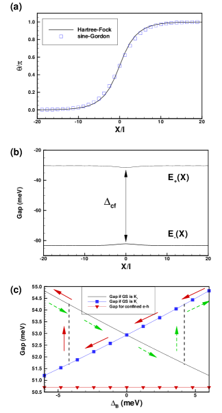
Figure 3: (Color online) Domain wall for $\Delta_{B}=0,N=-1,B=10T$ and hysteretic behavior. (a) Comparison of the sine-Gordon and Hartree-Fock solutions. (b) Band structure, $E_{\pm}\left(X\right)$ in the domain wall solution. The gap for a confined electron-hole excitation is indicated by $\Delta_{\mathrm{cf}}.$ (c) Hysteretic behavior of the transport gap around zero bias. The plain (dashed) arrows indicate the progression of the gap for a downward (upward) sweep in bias.

It is interesting to compare the Hartree-Fock solution with the DW solution that can be obtained by solving the Euler-Lagrange equationsolyom derived from the energy functional of Eq. (III.4.2). Neglecting the capacitive term and at zero bias, the excitation energy is

$$\delta E_{\mathrm{valley}} = \frac{1}{2}L_{y}\int dx\left[\rho_{z}\sin^{2}\theta+\rho_{\bot}\cos^{2}\theta\right]\left(\partial_{x}\theta\right)^{2}$$

$$+KL_{y}\int dx\cos^{2}\theta.$$

Considering a Néel wall and neglecting the small difference between the stiffnesses $\rho_{z}$ and $\rho_{\bot}$ at zero bias, the Euler-Lagrange equation simplifies to the sine-Gordon equation

$$\frac{\partial^{2}\varphi}{\partial x^{2}}=\frac{1}{\lambda^{2}}\sin\left(\varphi\right),$$ (99)

where $\varphi=2\theta$ and

$$\lambda=\sqrt{\frac{\rho_{z}}{2\left|K\right|}}.$$ (100)

Imposing the boundary conditions $\theta\left(x=-\infty\right)=0$ and $\theta\left(x=\infty\right)=\pi,$ a solution that minimizes the energy is the sine-Gordon solitonrajaraman

$$\theta_{\mathrm{SG}}\left(x\right)=2\arctan\left(e^{\frac{x}{\lambda}}\right),$$ (101)

where $\lambda$ is the domain wall width (i.e. the coherence region). Note that, in the sine-Gordon solution, $p_{z}(q_{x}=0)=0$ and the capacitive term can effectively be neglected.

In Fig. 3(a), the Hartree-Fock and sine-Gordon DW solutions for $N=-1,\Delta_{B}=0$ and $B=10$ T are compared. The sine-Gordon solution is actually very close to the Hartree-Fock result. The domain wall width extracted from Eq. (101) is $\lambda=3.16\ell$. This is much larger than the domain wall width found in AlAs quantum wellsjungwirth .

VII EXCITATION GAP FOR SKYRMION-ANTISKYRMION PAIRS

VII.1 Hamiltonian in the symmetric gauge

To compute the skyrmion excitations, it is more convenient to use the symmetric gauge $\mathbf{A}=\left(By/2,-Bx/2\right)$ with $\mathbf{B}=-B\widehat{z}$ instead of the Landau gauge. The Landau gauge wave functions $h_{n,X}\left(\mathbf{r}\right)$ in the spinors of Eqs. (2)-(3) are then be replaced by the functions $\Phi_{n,m}\left(\mathbf{r}\right)$ where the quantum number $m=0,1,2,...$ is related to the angular momentum $l_{z}$ by $l_{z}=\left(m-n\right)\hslash.$ The functions $\Phi_{n,m}\left(\mathbf{r}\right)$ are given byyoshioka (by definition, $\Phi_{n,m}\left(\mathbf{r}\right)=0$ if $n<0$ or $m<0$)

$$\Phi_{n,m}\left(\mathbf{r}\right) = B_{n,m}e^{i\left(m-n\right)\varphi}\left(\frac{r}{\ell}\right)^{\left|m-n\right|}e^{-\frac{r^{2}}{4\ell^{2}}}$$

$$\times L_{\frac{n+m}{2}-\frac{\left|n-m\right|}{2}}^{\left|m-n\right|}\left(\frac{r^{2}}{2\ell^{2}}\right),$$

where $\varphi$ is the angle between the vector $\mathbf{r}$ and the $x$ axis, $L_{n}^{m}\left(x\right)$ is a generalized Laguerre polynomial and the normalization constant is given by

$$B_{n,m}=\frac{C_{n,m}\left(-i\right)^{n}}{\sqrt{2^{\left|m-n\right|}2\pi\ell^{2}}}\sqrt{\frac{\left(\frac{n+m}{2}-\frac{\left|n-m\right|}{2}\right)!}{\left(\frac{n+m}{2}+\frac{\left|n-m\right|}{2}\right)!}}$$ (103)

withnote3 $C_{n,m}=1$ if $m\geq n$ and $C_{n,m}=\left(-1\right)^{m-n}$ if $m<n$.

In the Hartree-Fock approximation, the Hamiltonian in the symmetric gauge is given by

$$H_{HF} = \sum_{\mu,m}\left(E_{\mu_{\xi}}^{\left(0\right)}-\mu_{\sigma}\Delta_{Z}\right)c_{\mu,m}^{{\dagger}}c_{\mu,m}$$

$$-\sum_{\mu}\sum_{m_{1},m_{2}}U_{m_{1},m_{1},m_{2},m_{2}}^{\gamma_{\xi},\gamma_{\xi},\mu_{\xi},\mu_{\xi}}c_{\mu,m_{2}}^{{\dagger}}c_{\mu,m_{2}}$$

$$+\sum_{\mu,\nu}\sum_{m_{1},\ldots,m_{4}}U_{m_{1},m_{2},m_{3},m_{4}}^{\mu_{\xi},\mu_{\xi},\nu_{\xi},\nu_{\xi}}\left(\left\langle c_{\mu,m_{1}}^{{\dagger}}c_{\mu,m_{2}}\right\rangle\right.$$

$$\left.\times c_{\nu,m_{3}}^{{\dagger}}c_{\nu,m_{4}}-\left\langle c_{\mu,m_{1}}^{{\dagger}}c_{\nu,m_{4}}\right\rangle c_{\nu,m_{3}}^{{\dagger}}c_{\mu,m_{2}}\right),$$

where the matrix elements of the Coulomb interaction are defined by

$$U_{m_{1},m_{2},m_{3},m_{4}}^{\mu_{\xi},\mu_{\xi},\nu_{\xi},\nu_{\xi}} = \sum_{i,j=1}^{4}\left|b_{\mu_{\xi},i}\right|^{2}\left|b_{\nu_{\xi},j}\right|^{2}$$

$$\times V\left(i,j\right)_{m_{1},m_{2},m_{3},m_{4}}^{\left(\alpha_{\mu_{\xi}}\right)_{i},\left(\alpha_{\mu_{\xi}}\right)_{i},\left(\alpha_{\nu_{\xi}}\right)_{j},\left(\alpha_{\nu_{\xi}}\right)_{j}},$$

with

$$\alpha_{-1} = \left(n-1,n,n-2,n-1\right),$$ (106)

$$\alpha_{+1} = \left(n-1,n-2,n,n-1\right),$$ (107)

and

$$V\left(i,j\right)_{m_{1},m_{2},m_{3},m_{4}}^{n,n,n^{\prime},n^{\prime}}$$

$$= \left(\frac{e^{2}}{\kappa\ell}\right)\delta_{m_{1}-m_{2}+m_{4}-m_{3}}$$

$$\times\sqrt{\frac{\min\left(m_{1},m_{2}\right)!\min\left(m_{3},m_{4}\right)!}{\max\left(m_{1},m_{2}\right)!\max\left(m_{3},m_{4}\right)!}}$$

$$\times\int_{0}^{\infty}dke^{-k^{2}}e^{-\Delta\left(i,j\right)kd/\ell}\left(\frac{k^{2}}{2}\right)^{\left|m_{1}-m_{2}\right|}L_{n}^{0}\left(\frac{k^{2}}{2}\right)$$

$$\times L_{n^{\prime}}^{0}\left(\frac{k^{2}}{2}\right)L_{\min(m_{1},m_{2})}^{\left|m_{1}-m_{2}\right|}\left(\frac{k^{2}}{2}\right)L_{\min(m_{3},m_{4})}^{\left|m_{3}-m_{4}\right|}\left(\frac{k^{2}}{2}\right),$$

where $\Delta\left(i,j\right)=0$ or $1$ when $\left|i-j\right|\leq 1$ or $\left|i-j\right|\geq 2.$ The Hamiltonian $H_{HF}$ includes an interaction with a positive background where the positive charges are assumed to occupy the same state, $\gamma,$ as the electrons in the ground state.

VII.2 Spin and valley-pseudospin skyrmions

At $\nu_{N}=1,$ the ground state has $\mu=1$ or $\mu=3$ and can be written as

$$\left|\mathrm{GS}\right\rangle=\prod\limits_{m=0}c_{\mu,m}^{{\dagger}}\left|0\right\rangle.$$ (109)

If, for example, $\mu=1,$ then a general antiskyrmion (one electron removed from the ground state) that allows for the possibility of an intertwined spin and valley-pseudospin textures can be written as

$$\left|\mathrm{aSk}\right\rangle=\prod\limits_{m=0}\xi_{m}^{{\dagger}}\left|0\right\rangle,$$ (110)

where the operator

$$\xi_{m}^{{\dagger}} = u_{1,m}c_{1,m+1}^{{\dagger}}+u_{2,m}c_{2,m}^{{\dagger}}$$

$$+u_{3,m}c_{3,m}^{{\dagger}}+u_{4,m}c_{4,m}^{{\dagger}}.$$

For a skyrmion (one electron added to the ground state), three types of excitations are possibleezawa depending on the level the extra electron is added to i.e.:

$$\left|\mathrm{Sk}\right\rangle_{k}=\prod\limits_{m=0}\xi_{k,m}^{{\dagger}}c_{k,0}^{{\dagger}}\left|0\right\rangle,$$ (112)

with $k=2,3,4$ and

$$\xi_{2,m}^{{\dagger}} = u_{1,m}c_{1,m}^{{\dagger}}+u_{2,m}c_{2,m+1}^{{\dagger}}$$

$$+u_{3,m}c_{3,m}^{{\dagger}}+u_{4,m}c_{4,m}^{{\dagger}},$$

$$\xi_{3,m}^{{\dagger}} = u_{1,m}c_{1,m}^{{\dagger}}+u_{2,m}c_{2,m}^{{\dagger}}$$

$$+u_{3,m}c_{3,m+1}^{{\dagger}}+u_{4,m}c_{4,m}^{{\dagger}},$$

$$\xi_{4,m}^{{\dagger}} = u_{1,m}c_{1,m}^{{\dagger}}+u_{2,m}c_{2,m}^{{\dagger}}$$

$$+u_{3,m}c_{3,m}^{{\dagger}}+u_{4,m}c_{4,m+1}^{{\dagger}}.$$

The normalization condition imposes $\sum_{\mu}\left|u_{\mu,m}\right|^{2}=1$ for each $m.$ A similar scheme is applied if the ground state has $\mu=3.$

When the coefficients $u_{\mu,m}=0$ for $\mu=2,3,4,$ the antiskyrmion or skyrmion excitations are reduced to the bulk hole $\left|\mathrm{h}\right\rangle=c_{1,0}\left|\mathrm{GS}\right\rangle$ or bulk electron excitations $\left|\mathrm{e}\right\rangle_{k}=c_{k,0}^{{\dagger}}\left|\mathrm{GS}\right\rangle$ respectively. If $u_{2,m}=u_{4,m}=0,$ the excitation is a pure valley-pseudospin skyrmion, $\left|\mathrm{VSk}\right\rangle,$ or valley-pseudospin antiskyrmion, $\left|\mathrm{VaSk}\right\rangle,$ with spin $\sigma=+1.$ If $u_{3,m}=u_{4,m}=0$ (or $u_{1,m}=u_{2,m}=0$), the excitation is a pure spin-skyrmion, $\left|\mathrm{SSk}\right\rangle,$ or spin-antiskyrmion, $\left|\mathrm{SaSk}\right\rangle,$ in valley $K_{+}$ (or $K_{-}$).

To compute the coefficients $u_{p,m}$ for the antiskyrmion excitation, we define the $4\times 4$ matrix of Green’s functions $G_{m}\left(\tau\right)=-\left\langle Tv_{m}\left(0\right)v_{m}^{{\dagger}}\left(\tau\right)\right\rangle$ where $v_{m}=\left(\begin{array}[]{cccc}c_{1,m+1}&c_{2,m}&c_{3,m}&c_{4,m}\end{array}\right)^{{\dagger}}$ and write down its Hartree-Fock equation of motion using the Hamiltonian of Eq. (VII.1). The procedure is described in detail in Ref. luo2, and is equivalent to the canonical transformation method used to compute spin-skyrmion in Ref. fertig, . The resulting self-consistent equation for the matrix Green’s function is solved numerically in an iterative way until a converging solution is found. We proceed in a similar way for the three skyrmion excitations. The occupation of each quantum state $m$ is given by $\left|u_{\mu,m}\right|^{2}$ and the coherence factors by $u_{\mu,m}u_{\nu,m}^{\ast}$ ($\mu\neq\nu$). These coherences are responsible for the spin and valley-pseudospin textures. They are obtained from the off-diagonal elements of the matrix $G_{m}\left(\tau=0^{-}\right)$. In the numerical calculation, the maximum value of $m$ is set to $m_{\max}=500$ so that skyrmions up to $R\approx\sqrt{2m_{\max}}\ell$ in size can be obtained.

For a pure spin skyrmion, the number of flipped spins per skyrmion when the ground state has electrons with spin $\sigma=+1$ in valley $\xi=1$ or $-1$ is given by

$$K_{\mathrm{spin}}=\sum_{m}\left|u_{2\text{ }\mathrm{or}\text{ }4,m}\right|^{2},$$ (116)

while the number of flipped valley pseudospins per skyrmion is

$$K_{\mathrm{pspin}}=\sum_{m}\left|u_{3\text{ }\mathrm{or}\text{ }1,m}\right|^{2}.$$ (117)

VII.3 Numerical results for skyrmions

We choose $\mu=1$ for the ground state at zero bias. Figure 4(a) shows the excitation energies of the antiskyrmion and bulk hole as a function of the Zeeman coupling for Landau level $N=-1$. Note that, with a maximum number of angular momenta $m_{\max}=500$, we are limited to the range $\Delta_{Z}\geq 0.14$ meV otherwise the skyrmion is too big. Figure 4 shows that the antiskyrmion has lower energy than the bulk hole in the small Zeeman range $\Delta_{Z}\in\left[0,1.28\right]$ meV. There is no intertwined spin-valley pseudospin texture in this range. Indeed, for $\Delta_{Z}\lesssim 0.85$ meV, the excitation is a pure spin antiskyrmion, $\left|\text{{SaSk}}\right\rangle,$ while above this value it is a pure valley-pseudospin antiskyrmion,$\left|\text{{VaSk}}\right\rangle$. The corresponding number of spin flips $K_{\mathrm{spin}}$ or valley-pseudospin flips $K_{\mathrm{pspin}}$ is shown in Fig. 5(a) as a function of the Zeeman coupling. Naturally, $K_{\mathrm{pspin}}$ is independent of the Zeeman coupling while $K_{\mathrm{spin}}$ increases with decreasing $\Delta_{Z}.$

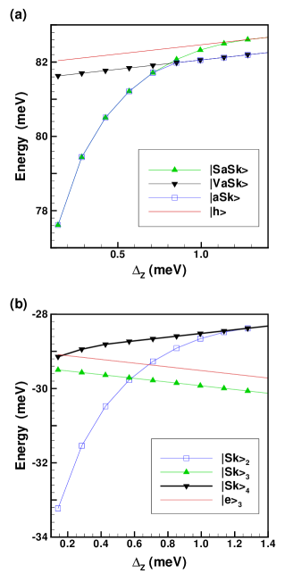
Figure 4: (Color online) Excitation energy at zero bias of the (a) antiskyrmion and bulk quasi-hole; (b) skyrmion and bulk quasi-electron as a function of the Zeeman coupling for Landau level $N=-1$ and magnetic field $B=10$ T.

Figure 4(b) shows the excitation energy for the skyrmion and bulk electron states for $N=-1$ and zero bias. The state $\left|\mathrm{e}\right\rangle_{3}$ has the lowest energy amongst the bulk electron states since the two other bulk states $\left|\mathrm{e}\right\rangle_{2}$ and $\left|\mathrm{e}\right\rangle_{4}$ (not shown in the figure) are degenerate and involve a spin flip. The lowest-energy skyrmion is $\left|\mathrm{Sk}\right\rangle_{2}$ for $\Delta_{Z}<0.59$ meV and $\left|\mathrm{Sk}\right\rangle_{3}$ above this value. The transition between these two skyrmion types is discontinuous. Again, no intertwined texture is found. The excitation $\left|\mathrm{Sk}\right\rangle_{2}$ and $\left|\mathrm{Sk}\right\rangle_{3}$ are respectively a spin and a valley-pseudospin skyrmion. Apart from a global Zeeman shift of their energy due to added or removed electron, the energy of the valley-pseudospin skyrmion and antiskyrmion is independent of the Zeeman coupling since these excitations do contain spin flip. Moreover, the coefficients of the eigenspinors in Eqs. (2-3) do not depend on the Zeeman coupling either. The number of spin flips for $\left|\mathrm{Sk}\right\rangle_{2}\left(\left|\mathrm{Sk}\right\rangle_{3}\right)$ is identical to that for $\left|\text{{SaSk}}\right\rangle\left(\left|\text{{VaSk}}\right\rangle\right)$.

The sum of the skyrmion and antiskyrmion energies gives the energy needed to create a skyrmion-antiskyrmion pair with an infinite separation. At zero Zeeman coupling, the spin skyrmion-antiskyrmion pair has lower energy than the bulk electron-hole pair in the range $\Delta_{Z}\in\left[0,1.28\right]$ meV. In graphene however, $\Delta_{Z}=1.16$ meV if the magnetic field is not tilted. At this value, the relevant excitations for the transport gap (i.e. the pair excitations with the lowest energy) are the valley-pseudospin skyrmion-antiskyrmion pairs.

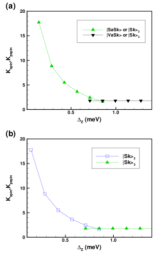
Figure 5: (Color online) Number of spin flips ($K_{\mathrm{spin}}$) or valley pseudospin flips ($K_{\mathrm{pspin}}$) as a function of the Zeeman coupling for the lowest-energy excitations in Fig. 4.

To study the valley-pseudospin skyrmions as a function of bias, we take $\Delta_{Z}=2.1$ meV, i.e. a value large enough to kill the spin texture. The ground state for $N\leq-1$ has $\mu=3$ for $\Delta_{B}>0$ and $\mu=1$ for $\Delta_{B}<0$. We find a pure valley-pseudospin skyrmion in this case: $\left|\mathrm{Sk}\right\rangle_{1}$ for $\Delta_{B}>0$ and $\left|\mathrm{Sk}\right\rangle_{3}$ for $\Delta_{B}<0.$ The excitation energy of valley-pseudospin antiskyrmion and skyrmion is plotted in Fig. 6 (a) and (b) together with the energy of the corresponding bulk electron and hole. The valley-pseudospin texture gradually disappears as $\left|\Delta_{B}\right|$ increases. The range of bias where the topological excitations win over the bulk ones is small: $\left|\Delta_{B}\right|\leq 1.77$ meV and $\left|\Delta_{B}\right|\leq 1.42$ meV respectively. The number of valley-pseudospin flips, $K_{\mathrm{pspin}}$ is shown in Fig. 7. It is maximal at zero bias and decreases rapidly with increasing bias. At zero bias, $K_{\mathrm{pspin}}\approx 2,$ and so these skyrmions are very small in space unlike the spin skyrmions at zero Zeeman coupling.

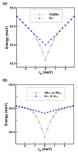
Figure 6: (Color online) Excitation energy of (a) valley antiskyrmion and quasi-hole; (b) valley skyrmion and quasi-electron for bias $\Delta_{B}=0.03e^{2}/\kappa\ell,$ $B=10$ T and $N=-1.$ The excitations are $\left|e\right\rangle_{1}$ and $\left|Sk\right\rangle_{1}$ for positive bias and $\left|e\right\rangle_{3}$ and $\left|Sk\right\rangle_{3}$ for negative bias.

The induced density profiles $\delta n\left(\mathbf{r}\right)=n\left(\mathbf{r}\right)-n_{GS}\left(\mathbf{r}\right)$ of the spin and valley-pseudospin skyrmions or antiskyrmions are similar to that of spin skyrmions in a semiconductor 2DEGezawa . The density $\delta n\left(\mathbf{r}\right)$ is maximal and positive at the origin for a skyrmion (or minimal and negative for an antiskyrmion). It is isotropic and decreases(increases) to zero at infinity for skyrmion(antiskyrmion). The integrated density $\int d\mathbf{r}\delta n\left(\mathbf{r}\right)$ contains one more(less) electron for a skyrmion(antiskyrmion). A plot of the valley-pseudospin texture in the projected representation, which is defined in Appendix A, gives the pattern represented in Fig. 8. The pairing with $\Delta m=\pm 1$ in Eqs. (VII.2)-(VII.2) leads to a spin or valley-pseudospin vortex around the origin where the pseudospins rotate by $\pm 2\pi$.

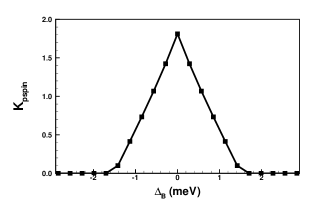
Figure 7: Number of flipped valley pseudospins per skyrmion or antiskyrmion as a function of bias in Landau level $N=-1$ and magnetic field $B=10$ T.

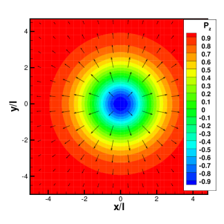
Figure 8: (Color online) Valley-pseudospin texture of a valley-pseudospin skyrmion in Landau level $N=-1$ and magnetic field $B=10$ T in the projected representation.

Figure 9 shows the energy of the different pair excitations in Landau level $N=-1$ with $B=10$ T and in level $N=1$ with $B=21$ T with the Zeeman coupling $\Delta_{Z}=g\mu_{B}B$ in both cases. Spin skyrmion-antiskyrmion pairs are not relevant at these Zeeman couplings and so only the bulk and confined electron-hole pairs and the valley-pseudospin skyrmion-antiskyrmion pairs are considered. From this figure, it is clear that, if domain walls are present, then the confined pairs are the relevant excitations at small bias. Otherwise, skyrmion-antiskyrmion pairs win but their energy is only slightly lower than that of the bulk quasiparticles.

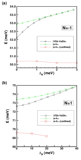
Figure 9: (Color online) Energy with bias of bulk and confined electron-hole pairs and of valley-pseudospin skyrmion-antiskyrmion pairs. (a) $N=-1,B=10$ T ; (b) $N=1,B=21$ T.

We were not able to obtain spin or valley-pseudospin skyrmions in Landau levels $\left|N\right|>1$. For the spin skyrmions, it was foundluo2 that in graphene (monolayer), the range of Zeeman coupling where skyrmions are the lowest-energy excitations decreases very rapidly with increasing $\left|N\right|.$ We assume that the same behavior applies to bilayer graphene and that, if skyrmions exist (according to the nonlinear $\sigma$ model discussed in the next section, they do for some higher values of $\left|N\right|$), then they do so in a Zeeman range not accessible to our numerical approach. For valley-pseudospin skyrmions, the number of pseudospin flips shown in Fig. 8 indicates that they are very small. Increasing the Landau level index will make them even smaller, indistinguishable from the bulk charged excitations.

VII.4 Spin skyrmion in the gradient approximation

It may seem surprising that the excitation energy of the spin skyrmion is lower than that of the valley-pseudospin skyrmion at small Zeeman coupling and zero bias (see Fig. 4) since, in the non-interacting picture, there is no cost for a valley pseudospin flip and the exchange-energy cost seems similar in the two excitations. However, as shown in Sec. III, the energy functional in the gradient approximation is very different for spin and valley-pseudospin textures. For valley pseudospins, the exchange interaction is anisotropic and there is an easy-axis anisotropy term and an easy-plane term (the capacitive energy).

In the limit $\Delta_{Z}\rightarrow 0,$ skyrmions have a slowly-varying spin texture and their excitation energy can be computed from the nonlinear $\sigma$ model (NL$\sigma$M) energy functional in Eq. (54). The energy needed to create a spin skyrmion-antiskyrmion pair with infinite separation issondhi ; moon

$$E_{SSk-SaSk}^{NL\sigma M}=8\pi\rho_{S},$$ (118)

where the spin stiffness is defined in Eq. (55). This value provides a lower bound for the Hartree-Fock calculations shown in Fig. 4 since the limit $\Delta_{Z}\rightarrow 0$ cannot be reached numerically. According to Eq. (118), a spin skyrmion-antiskyrmion pair at zero Zeeman and zero bias has an energy lower than a bulk electron-hole pair for $N\in\left[-3,-1\right]$ and $N\in\left[1,4\right]$ at $B=10$ T. Table 1 lists the value of these two gap energies for different Landau levels.

$N$	$E_{\left(e-h\right),spin}^{Bulk}$ (meV)	$E_{SSk-SaSk}^{NL\sigma M}$ (meV)
$\pm 1$	$\begin{array}[]{c}51.1\\ 52.9\end{array}$	$\begin{array}[]{c}24.2\\ 24.5\end{array}$
$\pm 2$	$\begin{array}[]{c}43.2\\ 43.9\end{array}$	$\begin{array}[]{c}28.8\\ 31.4\end{array}$
$\pm 3$	$\begin{array}[]{c}38.9\\ 39.3\end{array}$	$\begin{array}[]{c}31.5\\ 35.0\end{array}$
$\pm 4$	$\begin{array}[]{c}36.0\\ 36.2\end{array}$	$\begin{array}[]{c}33.5\\ 37.4\end{array}$
$\pm 5$	$\begin{array}[]{c}33.8\\ 34.0\end{array}$	$\begin{array}[]{c}35.3\\ 39.4\end{array}$

Table 1: Energy of a bulk electron-hole pair and a spin skyrmion-antiskyrmion pair in the NL$\sigma$M calculated as a function the Landau level index $N$ at zero bias and zero Zeeman coupling and at $B=10$ T. The results are the same in the two valleys. In each entry, the upper(lower) value is for the positive(negative) values of $N$.

VII.5 Valley skyrmion in the gradient approximation

If the easy-axis anisotropy and capacitive terms could be neglected in the anisotropic nonlinear $\sigma$ model (ANL$\sigma$M) energy functional of Eq. (III.4.2), then the valley-pseudospin skyrmion-antiskyrmion excitation (or bimeron-antibimeron) energy would be given by brey

$$E_{VSk-VaSk}^{ANL\sigma M}=\frac{16\pi}{3}\rho_{\bot}+\frac{8\pi}{3}\rho_{z}$$ (119)

and the number of valley-pseudospin flips would diverge at zero bias. As our microscopic calculations shows, this does not happen. Valley-pseudospin skyrmions have a finite small size at zero bias and so Eq. (119) cannot be used to compute their energies. It is necessary to include the capacitive and easy-axis term as well as the Hartree energy due to the density modulation induced by the skyrmions. All these terms are included in our microscopic Hartree-Fock calculation of the skyrmion energy.

Inter-Landau-level spin-skyrmions have been studied before in semiconductor quantum wellslilliehook but it was shown that are never the lowest-lying charged excitations. By contrast, we find here, in bilayer graphene, that skyrmions where different orbitals (but of the same Landau level) are mixed can be the lowest-lying charged excitations.

VIII CONCLUSION

We have computed the energy of different types of pair excitations in the Ising quantum Hall ferromagnetic states of bilayer graphene in Landau levels $\left|N\right|>0$. These excitations include bulk electron-hole pairs, electron-hole pairs confined to the coherent region of a domain wall, and skyrmions-antiskyrmion pairs. For a disorder-free systems where the Coulomb interaction is treated in the Hartree-Fock approximation, valley-pseudospin skyrmion-antiskyrmion pairs have a lower excitation energy than bulk electron-hole pairs. At finite temperature or in a disordered system where domain walls are created, confined electron-hole pairs are the lowest-energy excitations but only in a small range of bias.

When confined electron-hole pairs are excited, it should be possible, according to the theory developed in Ref. jungwirth, to observe a breakdown of the quantum Hall effect. In previously studied Ising systems in semiconductor quantum wells, this breakdown lead to the apparition of magnetoresistance spikes near the Ising transitions. These spikes were observed experimentallypoortere . According to Ref. jungwirth, , when the chemical potential is pinned in the bulk quasiparticle energy, the confined electron-hole pairs can be easily excited. If the domain wall loops are dense enough to overlap, these confined quasiparticles can cross the sample by scattering from one loop to an adjacent one and then increase the dissipation in the sample, creating magnetoresistance spikes that are detected near integer fillings close to the transition between the ordered and the paramagnetic phases at finite temperature. As far as we know, there has been to date no experimental study of such effect in the higher Landau levels of bilayer graphene.

The domain wall solution discussed in this work comes from the Coulomb interaction. It is different from the domain walls studied before in bilayer graphenefertig1 which were artificially created in the middle of a double-gated bilayer graphene sample by placing it in an electric gate where the potential profile changes sign across the centermartin . Domain walls have also recently been studied in bilayer graphene but at zero magnetic fieldli .

Another type of excitation should be considered in addition to those studied in this work. It consists of confined textured excitations in the coherent regions of the domain walls i.e. confined solitons and antisolitons of the valley pseudospin in the one-dimensional coherent region of a wall. It is possible to extract an effective pseudospin Hamiltonian for such excitations by combining the long-wavelength energy functional presented in this paper with the microscopic Hartree-Fock calculation. This has been done previously in Ising QHFsbrey ; jungwirth ; muraki ; falko and in the coherent stripe phase in a semiconductor double quantum-well systemdoiron . We leave this problem to future work.

Appendix A PROJECTED REPRESENTATION IN THE SYMMETRIC GAUGE

The total density in Landau level $N$ is given by

$$\widetilde{n}\left(\mathbf{r}\right)=\sum_{\mu}\int dz\left\langle\Psi_{\mu}^{{\dagger}}\left(\mathbf{r},z\right)\Psi_{\mu}\left(\mathbf{r},z\right)\right\rangle.$$ (120)

In the absence of valley coherence, the spin density field in real space is given by

$$\widetilde{S}_{z}\left(\mathbf{r}\right)=\frac{1}{2}\sum_{\mu}\mu_{\sigma}\int dz\left\langle\Psi_{\mu}^{{\dagger}}\left(\mathbf{r},z\right)\Psi_{\mu}\left(\mathbf{r},z\right)\right\rangle,$$ (121)

and

$$\widetilde{S}_{x}\left(\mathbf{r}\right)+i\widetilde{S}_{y}\left(\mathbf{r}\right) = \sum_{\xi}\int dz$$

$$\times\left\langle\Psi_{\xi,+}^{{\dagger}}\left(\mathbf{r},z\right)\Psi_{\xi,-}\left(\mathbf{r},z\right)\right\rangle.$$

Similarly, in the absence of spin coherence, the valley-pseudospin field given in real space by

$$\widetilde{P}_{z}\left(\mathbf{r}\right)=\frac{1}{2}\sum_{\mu}\mu_{\xi}\int dz\left\langle\Psi_{\mu}^{{\dagger}}\left(\mathbf{r},z\right)\Psi_{\mu}\left(\mathbf{r},z\right)\right\rangle,$$ (123)

and

$$\widetilde{P}_{x}\left(\mathbf{r}\right)+i\widetilde{P}_{y}\left(\mathbf{r}\right) = \sum_{\sigma}\int dz$$

$$\times\left\langle\Psi_{+,\sigma}^{{\dagger}}\left(\mathbf{r},z\right)\Psi_{-,\sigma}\left(\mathbf{r},z\right)\right\rangle.$$

These density and fields contain the character of the different Landau level orbitals $n$ in $\Phi_{n,m}\left(\mathbf{r}\right)$ that enter the definition of the spinors in Eq. (2,3) with the wave functions in the symmetric gauge. Since these spinors contain a mixture of the orbitals $n,n-1$ and $n-2,$ the resulting field pattern of a skyrmion in real space is complex. To get a simpler visualization of the spin and pseudospin fields, it is useful to use a projected representation that we define in the following way. We write

$$\Lambda_{\mu,\mu^{\prime}}\left(\mathbf{r}\right) = \int dz\Psi_{\mu}^{{\dagger}}\left(\mathbf{r},z\right)\Psi_{\mu^{\prime}}\left(\mathbf{r},z\right)$$

$$= \sum_{m_{1},m_{2}}\Gamma_{m_{1},m_{2}}^{\mu_{\xi},\mu_{\xi}^{\prime}}\left(\mathbf{r}\right)c_{\mu,m_{1}}^{{\dagger}}c_{\mu^{\prime},m_{2}},$$

where, for example,

$$\Gamma_{m_{1},m_{2}}^{+,+}\left(\mathbf{r}\right) = b_{+,1}^{\ast}b_{-,1}\Phi_{n-1,m_{1}}^{\ast}\left(\mathbf{r}\right)\Phi_{n-1,m_{2}}\left(\mathbf{r}\right)$$

$$+b_{+,2}^{\ast}b_{-,2}\Phi_{n-2,m_{1}}^{\ast}\left(\mathbf{r}\right)\Phi_{n,m_{2}}\left(\mathbf{r}\right)$$

$$+b_{+,3}^{\ast}b_{-,3}\Phi_{n,m_{1}}^{\ast}\left(\mathbf{r}\right)\Phi_{n-2,m_{2}}\left(\mathbf{r}\right)$$

$$+b_{+,4}^{\ast}b_{-,4}\Phi_{n-1,m_{1}}^{\ast}\left(\mathbf{r}\right)\Phi_{n-1,m_{2}}\left(\mathbf{r}\right)$$

and the other components are easily obtained from the spinors in Eqs. (2,3). We define the Fourier transform of $\Gamma_{m_{1},m_{2}}^{\xi,\xi^{\prime}}\left(\mathbf{r}\right)$ as

$$\Gamma_{m_{1},m_{2}}^{\xi,\xi^{\prime}}\left(\mathbf{q}\right)=\int d\mathbf{r}\Gamma_{m_{1},m_{2}}^{\xi,\xi^{\prime}}\left(\mathbf{r}\right)e^{-i\mathbf{q}\cdot\mathbf{r}}.$$ (127)

In the symmetric gauge, the matrix elements that enter the Fourier transform are given by

$$\int d\mathbf{r}\Phi_{n_{1},m_{1}}\left(\mathbf{r}\right)e^{-i\mathbf{q}\cdot\mathbf{r}}\Phi_{n_{2},m_{2}}\left(\mathbf{r}\right)$$

$$= \left(\pm i\right)^{\left|n_{1}-n_{2}\right|}\left[F_{n_{1},n_{2}}\left(-\mathbf{q}\right)\right]^{\ast}F_{m_{1},m_{2}}\left(-\mathbf{q}\right),$$

with

$$F_{n_{1},n_{2}}\left(\mathbf{q}\right) = \sqrt{\frac{Min\left(n_{1},n_{2}\right)!}{Max\left(n_{1},n_{2}\right)!}}e^{-\frac{1}{4}q^{2}\ell^{2}}$$

$$\times\left(\frac{\left(\pm q_{y}+iq_{x}\right)\ell}{\sqrt{2}}\right)^{\left|n_{1}-n_{2}\right|}L_{Min\left(n_{1},n_{2}\right)}^{\left|n_{1}-n_{2}\right|}\left(\frac{q^{2}\ell^{2}}{2}\right),$$

where the upper sign is for $n_{1}\geq n_{2}$ and the lower sign for $n_{1}<n_{2}$ and $L_{n}^{a}\left(x\right)$ is a generalized Laguerre polynomial. It follows that

$$\Gamma_{m_{1},m_{2}}^{+,+}\left(\mathbf{q}\right)=\Omega_{+,+}\left(-\mathbf{q}\right)F_{m_{1},m_{2}}\left(\mathbf{q}\right),$$ (130)

where $\Omega_{+,+}\left(\mathbf{q}\right)$ does not involve the quantum number $m$ and is given by

$$\Omega_{+,+}\left(\mathbf{q}\right) = b_{+,1}^{\ast}b_{-,1}\left[F_{n-1,n-1}\left(\mathbf{q}\right)\right]^{\ast}$$

$$-b_{+,2}^{\ast}b_{-,2}\left[F_{n-2,n}\left(\mathbf{q}\right)\right]^{\ast}$$

$$-b_{+,3}^{\ast}b_{-,3}\left[F_{n,n-2}\left(\mathbf{q}\right)\right]^{\ast}$$

$$+b_{+,4}^{\ast}b_{-,4}\left[F_{n-1,n-1}\left(\mathbf{q}\right)\right]^{\ast}.$$

We thus get

$$\Lambda_{\mu,\mu^{\prime}}\left(\mathbf{q}\right) = \sum_{m_{1},m_{2}}\Omega_{\mu_{\xi},\mu_{\xi}^{\prime}}\left(-\mathbf{q}\right)F_{m_{1},m_{2}}\left(-\mathbf{q}\right)$$

$$\times c_{\mu,m_{1}}^{{\dagger}}c_{\mu^{\prime},m_{2}}.$$

References

- (1) For a review of the C2DEG in bilayer graphene in Landau level , see for example: Yafis Barlas, Kun Yang, and A. H. MacDonald, Nanotechnology 23, 052001 (2012).
- (2) For a review of some of the properties of graphene and bilayer graphene, see for example: A. H. Castro Neto, F. Guinea, N. M. R. Peres, K. S. Novoselov and A. K. Geim, Rev. Mod. Phys. 81, 109 (2009); D. S. L. Abergel, V. Apalkov, J. Berashevich, K. Ziegler and Tapash Chakraborty, Advances in Physics 59, 261 (2010); M. O. Goerbig, Rev. Mod. Phys. 83, 1193 (2011);Edward McCann and Mikito Koshino, Rep. Prog. Phys. 76, 056503 (2013).
- (3) Wenchen Luo, R. Côté, and Alexandre Bédard-Vallée, Phys. Rev. B 90, 075425 (2014).
- (4) J. Lambert and R. Côté, Phys. Rev. B 87, 115415 (2013).
- (5) Gabriele F. Giuliani and J. J. Quinn, Phys. Rev. B 31, 6228 (1985).
- (6) T. Jungwirth and A. H. MacDonald, Phys. Rev. Lett. 87, 216801 (2001).
- (7) For a schematic representation of a charged and a neutral domain wall loop, see Fig. 3(a) of T. Jungwirth, A. H. MacDonald, E. H. Rezayi, Physica E 12, 1 (2002).
- (8) T. Jungwirth, S. P. Shukla, L. Smrčka, M. Shayegan, and A. H. MacDonald, Phys. Rev. Lett. 81, 2328 (1998).
- (9) A. J. Daneshvar, C. J. B. Ford, M. Y. Simmons, A. V. Khaetskii, A. R. Hamilton, M. Pepper, and D. A. Ritchie, Phys. Rev. Lett. 79, 4449 (1997).
- (10) Vincenzo Piazza, Vittorio Pellegrini, Fabio Beltram, Werner Wegscheider, Tomáš Jungwirth, and Allan H. MacDonald, Nature 402, 638 (1999).
- (11) T. Jungwirth, and A. H. MacDonald, Phys. Rev. B 63, 035305 (2000).
- (12) Kayoung Lee, Babak Fallahazad, Jiamin Xue, David C. Dillen, Kyounghwan Kim, Takashi Taniguchi, Kenji Watanabe, and Emmanuel Tutuc, Science 345, 58 (2014).
- (13) D. Lilliehöök, Phys. Rev. B 62, 7303 (2000).
- (14) Zyun F. Ezawa, Quantum Hall Effects: Field Theoretical Approach and Related Topics, Second Edition. World Scientific, Singapour (2007).
- (15) S. Ghosh and R. Rajaraman, Phys. Rev. B 63, 035304 (2000).
- (16) Wenchen Luo, R. Côté, Phys. Rev. B 88, 115417 (2013).
- (17) E. P. De Poortere, E. Tutuc, S. J. Papadakis, and M. Shayegan, Science 290, 1546 (2000).
- (18) The value of the hopping parameters that we use are those recently computed by Jeil Jung and Allan H. MacDonald, Phys. Rev. B 89, 035405 (2014). Our definition of the parameters differs by a minus sign from that used by these authors.
- (19) Edward McCann and Vladimir I. Fal’ko, Phys. Rev. Lett. 96, 086805 (2006).
- (20) R. Côté and Manuel Barrette, Phys. Rev. B 88, 245445 (2013).
- (21) K. Moon, H. Mori, Kun Yang, S. M. Girvin, A. H. MacDonald, L. Zheng, D. Yoshioka, and Shou-Cheng Zhang, Phys. Rev. B 51, 5138 (1995).
- (22) This is true in the gradient approximation but not in the microscopic Hartree-Fock approach unless the state is uniform or modulated in one direction of space only.
- (23) A. H. MacDonald and S. M. Girvin, Phys. Rev. B 34, 5639 (1986); R. Morf and B. I. Halperin, Phys. Rev. B 33, 2221 (1986).
- (24) For a similar calculation, see for ex.: Jenö Solyom, Fundamentals of the physics of solids, vol. 1 (Springer-Verlag, Berlin 2010).
- (25) R. Rajaraman, Solitons and instantons (North-Holland, Amsterdam 2003).
- (26) D. Yoshioka, The Quantum Hall Effect (Springer-Verlag, Berlin 2002).
- (27) In Ref. luo, , this is incorrectly written as if and if
- (28) H. A. Fertig, L. Brey, R. Côté, and A. H. MacDonald, Phys. Rev. B 50, 11018 (1994).
- (29) S. L. Sondhi, A. Karlhede, S. A. Kivelson, and E. H. Rezayi, Phys. Rev. B 47, 16419 (1993).
- (30) L. Brey, H. A. Fertig, R. Côté, and A. H. MacDonald, Phys. Rev. B 54, 16888 (1996).
- (31) Chia-Wei Huang, Efrat Shimshoni, and H. A. Fertig, Phys. Rev. B 85, 205114 (2012); Victoria Mazo, Chia-Wei Huang, Efrat Shimshoni, Sam T. Carr, and H. A. Fertig, Phys. Rev. B 89, 121411 (R) (2014).
- (32) Iva Martin, Ya. M. Blanter, and A. F. Morpurgo, Phys. Rev. Lett. 100, 036804 (2008).
- (33) Xiao Li, Fan Zhang, Qian Niu, and A. H. MacDonald, Phys. Rev. Lett. 113, 116803 (2014).
- (34) Koji Muraki, Tadashi Saku, and Yoshiro Hirayama, Phys. Rev. Lett. 87, 196801 (2001).
- (35) Vladimir I. Fal’ko and S. V. Iordanskii, Phys. Rev. Lett. 82, 402 (1999).
- (36) C. B. Doiron, R. Côté, and H. A. Fertig, Phys. Rev. B 72, 115336 (2005).