Numerical convergence in smoothed particle hydrodynamics

Abstract

We study the convergence properties of smoothed particle hydrodynamics (SPH) using numerical tests and simple analytic considerations. Our analysis shows that formal numerical convergence is possible in SPH only in the joint limit $N\rightarrow\infty$, $h\rightarrow 0$, and $N_{nb}\rightarrow\infty$, where $N$ is the total number of particles, $h$ is the smoothing length, and $N_{nb}$ is the number of neighbor particles within the smoothing volume used to compute smoothed estimates. Previous work has generally assumed that the conditions $N\rightarrow\infty$ and $h\rightarrow 0$ are sufficient to achieve convergence, while holding $N_{nb}$ fixed. We demonstrate that if $N_{nb}$ is held fixed as the resolution is increased, there will be a residual source of error that does not vanish as $N\rightarrow\infty$ and $h\rightarrow 0$. Formal numerical convergence in SPH is possible only if $N_{nb}$ is increased systematically as the resolution is improved. Using analytic arguments, we derive an optimal compromise scaling for $N_{nb}$ by requiring that this source of error balance that present in the smoothing procedure. For typical choices of the smoothing kernel, we find $N_{nb}\propto N^{0.5}$. This means that if SPH is to be used as a numerically convergent method, the required computational cost does not scale with particle number as $O(N)$, but rather as $O(N^{1+\delta})$, where $\delta\approx 0.5$, with a weak dependence on the form of the smoothing kernel.

1. Introduction

Smoothed particle hydrodynamics (SPH) has become a popular tool for studying astrophysical flows since its introduction in the mid-1970s by Lucy (1977) and Gingold & Monaghan (1977). Instead of solving the equations of hydrodynamics on a mesh, SPH operates by associating fluid elements with particles that characterize the flow. Local properties are estimated by “smoothing” the attributes of particles (neighbors) near a given point. Typically, the particles carry a fixed mass (unless converted to another form, such as collisionless stars), and the smoothing is done in a spherically symmetric manner using an interpolation function known as the smoothing kernel. Because it is gridless, SPH is naturally spatially adaptive if the scale of the smoothing, set by the smoothing length $h$, varies as the particles move with the flow. If individual particle timesteps are employed, the scheme will also be temporally adaptive.

SPH has been used with success especially in investigations of the formation and evolution of galaxies and large scale structure, where spatial and temporal adaptivity are essential because of the large range in scales present. Along with the successes has come an understanding of various limitations with SPH. Examples include: an artificial clumping instability for particular choices of the smoothing kernel (Schuessler & Schmitt, 1981); a lack of energy or entropy conservation for various forms of the equations of motion when the smoothing lengths vary spatially (Hernquist, 1993); and a poor handling of instabilities at shearing interfaces owing to artificial surface tension effects (Agertz et al., 2007). Many of the problems have already been overcome through a variety of improvements to the original formulation of SPH, such as the introduction of generalized smoothing kernels (Dehnen & Aly, 2012), fully conservative equations of motion based on variational principles (Springel & Hernquist, 2002), and various methods to eliminate artificial surface tension effects (Price, 2008; Read et al., 2010; Hopkins, 2013; Saitoh & Makino, 2013).

However, some issues remain unresolved, which has led to numerous misconceptions within the community of users of SPH. For example, because densities in SPH are calculated using smoothed estimates, rather than by solving the mass continuity equation, the flow of the fluid on small scales is not described correctly, as emphasized by Vogelsberger et al. (2012). One claimed advantage of SPH over grid based methods is that the previous history of fluid elements can be determined straightforwardly because individual particles retain their identity over time. With mesh codes, this can be accomplished only by introducing tracer particles into the flow so that the evolution of the density field can be reconstructed (Genel et al., 2013). In fact, this “advantage” of SPH owes to the fact that this method does not solve the equations of motion correctly on the smoothing scale.

Here, we focus on another issue with SPH that has received little attention in the literature, but for which confusion abounds: the numerical convergence of this technique. A commonly used approach for making SPH spatially adaptive is to allow the smoothing length of each particle to decrease or increase depending on the local density of particles. One possible choice is to scale the smoothing lengths in proportion to the mean interparticle separation according to $h\propto N^{-1/3}$ (Hernquist & Katz, 1989). A benefit to this scaling is that the number of particles used to compute smoothed estimates (particles neighboring a given point), $N_{nb}$, is roughly constant, optimizing the efficiency of the method from one region to another. But, this choice is somewhat arbitrary and leads to difficulties that are not widely recognized.

In SPH, local quantities are estimated by smoothing continuous fluid variables with an interpolation kernel. The resulting convolutions are evaluated numerically by approximating the integrals with discrete sums. These sums are calculated over $N_{nb}$ fluid elements (particles) near a given point. For the scaling noted above $N_{nb}\approx$ constant, and is typically limited to relatively small values $N_{nb}\approx 30-100$ to maximize spatial resolution. However, the approximation of the convolution integrals by discrete sums entails an error that depends directly on $N_{nb}$ and not $N$ or $h$. Therefore, as the resolution is improved by increasing $N$ and reducing $h$, numerical convergence is not possible because the error in the discrete estimates does not vanish if $N_{nb}$ is held constant.

Systematic studies of the convergence properties of SPH are lacking, but evidence that this source of error exists is present in the literature. For example, in his review of SPH, Springel (2010b) performed a series of tests to empirically determine the convergence rate of SPH. The behavior we suggest can be seen clearly in the Gresho vortex problem, as in Fig. 6 of Springel (2010b). Here, various runs were performed at improving resolution by increasing the total number of particles, $N$, and reducing the smoothing lengths, $h$, but holding the number of neighbors, $N_{nb}$ fixed. The solid curves in this figure compare the error in each case to a known analytic solution. For small particle numbers, increasing $N$ decreases the error, but eventually the error saturates and plateaus at value that depends in detail on the choice of artificial viscosity. However, if the runs with varying $N$ are compared to the highest resolution versions (dashed curves), the error shows a monotonically decreasing trend with $N$, for all choices of the artificial viscosity. This behavior can be explained only by the presence of a residual source of error that does not depend directly on $N$ and $h$. In what follows, we show that this error arises in the discrete sums used to approximate the local smoothing convolutions and that it depends directly only on the number of neighbors in these sums, $N_{nb}$.

For a random distribution of particles, this residual error essentially arises from shot noise in the discrete estimates and is expected to scale as $\propto N_{nb}^{-0.5}$. However, as emphasized by Monaghan (1992), SPH particles are usually not randomly distributed but are instead arranged in a “quasi-regular” pattern because of local forces between them. An analysis of the error in this situation suggests that the noise should scale with $N_{nb}$ as $\sim(d-1)N_{nb}^{-1}\log N_{nb}$, where $d$ is the number of dimensions. (Note that to this order of accuracy, the error estimate vanishes for $d=1$, meaning that 1-dimensional tests cannot be used to gauge the numerical convergence of SPH for $d>1$, contrary to common belief.)

Using simple numerical tests, we verify that the expected $\sim N_{nb}^{-1}\log N_{nb}$ behavior is a reasonable characterization of the discreteness error for multi-dimensional simulations with SPH. Therefore, the discreteness error, error_d, can be bounded by the estimates $N_{nb}^{-1}<$ error_d $<N_{nb}^{-0.5}$. Using this scaling, we suggest an optimal compromise between accuracy and efficiency by requiring that this error decline at the same rate as the error associated with the smoothing procedure itself, which directly involves only the smoothing lengths, $h$. In detail, the outcome depends on the form of the smoothing kernel, but for typical choices we find that the number of neighbors in the smoothed estimates should increase with the total particle number as $N_{nb}\propto N^{0.5}$. In this case, the smoothing lengths would scale as $h\propto N^{-1/6}$, rather than with the average separation between particles as $h\propto N^{-1/3}$, in which case $h$ represents the geometric mean of the size of the system and the average interparticle separation.

Our empirical tests verify that numerical convergence can indeed be obtained with SPH, if the neighbor number grows systematically with improved resolution. Of course, this comes with the consequence of increased computational expense relative to holding $N_{nb}$ fixed, and implies an unfavorable cpu scaling of $O(N^{3/2})$ compared to grid codes which are typically $O(N)$. This should not be surprising, since SPH is a Monte Carlo-like algorithm and it is well-known in other contexts that, while being flexible and general, Monte Carlo methods typically have unfavorable convergence properties relative to other more specialized techniques. Ultimately, applications with SPH must therefore choose between accuracy and computational efficiency. What is clear, however, is that if SPH is used with constant $N_{nb}$, numerical convergence is not possible.

We emphasize that this issue with the convergence of SPH is well-known in some disciplines (e.g. Robinson & Monaghan 2012). However, the specific problem we analyze here has been virtually ignored in discussions of the use of SPH in applications to cosmology and galaxy formation.

2. Consistency and Self-consistency

In SPH, densities are estimated from the particles by smoothing. This involves convolving a continuous field quantity, $A({\mathbf{r}})$, with a smoothing function $W(\mathbf{r},h)$ through

$$A_{s}(\mathbf{r})=\int A({\mathbf{r}})W(\mathbf{r}-\mathbf{r^{\prime}},h)d\mathbf{r}^{\prime},$$ (1)

where $A(\mathbf{r})$ and $A_{s}(\mathbf{r})$ denote the true field and its smoothed version. The smoothing length $h$ represents a characteristic width of the kernel over which the desired quantity is spread. The smoothing kernel is normalized to unity and asymptotically approaches a Dirac $\delta$-function when $h\rightarrow 0$. This can be achieved with a sufficiently large number of particles to describe the continuous system as $N\rightarrow\infty$.

Assuming that the volume within the smoothing kernel is sufficiently sampled with these discrete points, we can further approximate the above integral by discrete summations. The “volume” element $\Delta\mathbf{r}^{\prime}$ is estimated from $m_{b}/\rho_{b}$ where $m_{b}$ and $\rho_{b}$ are the mass and density of particle $b$ and we have

$$A_{d}(\mathbf{r})=\sum_{b}A_{b}\frac{m_{b}}{\rho_{b}}W(\mathbf{r-r}_{b},h).$$ (2)

With this approximation, we immediately obtain the density estimate in its discrete form $\rho_{d}(\mathbf{r})$ as used in SPH according to:

$$\rho_{d}(\mathbf{r})=\sum_{b}{m_{b}}W(\mathbf{r-r}_{b},h),$$ (3)

where the sum is over all the particles within the volume element centered at $\mathbf{r}$. A smoothing function with compact support is usually used to limit the “volume” to finite extent in order to minimize computation time. Equation (3) now operates on a finite number $N_{nb}$ of particles near a given point. In order to satisfy the consistency of this step, which is to approach the continuous limit with such finite summations, the condition $N_{nb}\rightarrow\infty$ is required.

Moreover, in applications with finite $N$ and $N_{nb}$, there is a lack of self-consistency based on the above approach. If we would represent a scalar field $A(\mathbf{r})$ with a constant value, say $1$, the following condition

$$1=\sum_{b}\frac{m_{b}}{\rho_{b}}W(\mathbf{r-r}_{b},h),$$ (4)

is generally not satisfied with the density field estimated from (3).

This lack of self-consistency is most extreme where large density gradients are present, e.g. between two phases of flow (Read et al., 2010) or close to a boundary (Liu & Liu, 2006). In other words, the volume estimate in SPH from equation (3) with a finite $N_{nb}$ is not an accurate partitioning of space. In order to satisfy the condition of consistency and self-consistency, the following conditions

$$N\rightarrow\infty,h\rightarrow 0,N_{nb}\rightarrow\infty$$ (5)

indeed should be met if no other fixes such as normalization are applied.

Next we discuss the consistency of the Euler equations that SPH actually solves. The original Euler equations in Lagrangian form describe the evolution of density, momentum, and internal energy according to:

$$\frac{d\rho}{dt}=-\rho\nabla\cdot\mathbf{v}$$ (6)

$$\frac{d\mathbf{v}}{dt}=-\frac{\nabla P}{\rho}$$ (7)

$$\frac{du}{dt}=-\frac{P}{\rho}\nabla\cdot\mathbf{v}$$ (8)

where $\rho$, $\mathbf{v}$ and $u$ represent the density, velocity, and internal energy per unit mass. The equation of state

$$P=u(\gamma-1)\rho$$ (9)

is a closure equation for the above system, where $\gamma$ is the adiabatic index of the gas. Following the derivation in Springel & Hernquist (2002), the equations of motion can be discretized as

$$\frac{d\rho_{a}}{dt}=f_{a}\sum_{b}m_{b}(\mathbf{v}_{a}-\mathbf{v}_{b})\cdot\nabla_{a}W(h_{a})$$ (10)

$$\frac{d\mathbf{v}_{a}}{dt}=-\sum_{b}m_{b}(\frac{f_{a}P_{a}}{\rho_{a}^{2}}\nabla_{a}W_{ab}(h_{a})+\frac{f_{b}P_{b}}{\rho_{b}^{2}}\nabla_{a}W_{ab}(h_{b}))$$ (11)

$$\frac{du_{a}}{dt}=f_{a}\frac{P_{b}}{\rho_{b}^{2}}\sum_{b}m_{a}(\mathbf{v}_{a}-\mathbf{v}_{b})\cdot\nabla_{a}W(h_{a}),$$ (12)

where the factors $f_{a}$ and $f_{b}$ depend on derivatives of the density with respect to the smoothing lengths. In practice instead of $u$, we can also use a variable $A(s)$ from $P=A(s)\rho^{\gamma}$ to solve the energy equation as in Springel & Hernquist (2002). These two approaches are equivalent in principle.

Read et al. (2010) have calculated the errors in the continuity and momentum equations with the above SPH formulation assuming a finite $N_{nb}$ (ignoring the factors $f_{a}$, which spoils the fully conservative nature of the equations) as

$$\frac{d\rho_{a}}{dt}\approx-\rho_{a}(\mathbf{R}_{a}\nabla_{a})\cdot\mathbf{v}_{a}+O(h)$$ (13)

$$\frac{d\mathbf{v}_{a}}{dt}\approx-\frac{P_{a}}{h\rho_{a}}\mathbf{E}_{0,a}-\frac{(\mathbf{V}_{a}\nabla_{a})P_{a}}{\rho_{a}}+O(h)$$ (14)

where $\mathbf{V}$, $\mathbf{R}$ are matrices close to the identity matrix $\mathbf{I}$ and $\mathbf{E}_{0}$ is a non-vanishing error vector. $\mathbf{V}$, $\mathbf{R}$ and $\mathbf{E}_{0}$ are all determined by the particle distribution within smoothing length $h$ (see Read et al. (2010) for detailed definitions). As a result, these errors will remain at the same level while we increase $N$ if $N_{nb}$ is fixed. However, a consistent scheme would require all the error terms in the above two equations go down as $h\rightarrow 0$. Similar conclusions can also be drawn for the energy equation.

Based on the above discussions of the density estimate and the discretized Euler equations in SPH, the condition $N_{nb}\rightarrow\infty$, $N\rightarrow\infty$ and $h\rightarrow 0$ has to be met in order to have a consistent and self-consistent scheme. Moreover, reducing $h$ will lead to finer time steps according to the CFL condition. If the magnitude of the error from a fixed $N_{nb}$ remains constant, the overall error will build up more rapidly in a high resolution run than a lower resolution one.

3. Error estimate of density estimate

The error in SPH from the smoothing procedure (independent of particle distribution) can be approximated to lowest order by:

$$error_{s}\propto h^{\alpha}.$$ (15)

For the usual B-splines (Monaghan, 2005; Price, 2012b) and the Wendland functions (Dehnen & Aly, 2012), this is a second order term where $\alpha$ = 2. Higher order precision can be achieved by constructing different classes of smoothing kernels. However, not all are appropriate since smoothed estimates of positive definite quantities can take on negative values.

The error from discretizing the integral convolutions in the smoothing procedure depends on whether or not particles are ordered in space. Optimistically, if the particles are quasi-ordered and not randomly distributed, it has been conjectured that the discretization error can be approximated by (Monaghan, 1992)

$$error_{d}\propto\frac{\log N_{nb}}{N_{nb}}.$$ (16)

This estimate is based on the study of the complexity associated with the low discrepancy sequence in numerical integration by Wozniakowski (1991). This indicates that the actual number of particles within the volume of each SPH particle should match the expected number of particles. Clearly, this is highly dependent on the randomness in the actual distribution of SPH particles.

The pressure force between SPH particles always tends to regulate the distribution of the SPH neighbors into an isotropic distribution. However, this “restoring” pressure force does not push the particles into an exact desired distribution since the number of neighbors is finite. Hence, the velocity field exhibits noise on small scales. Such velocity noise will further induce fluctuations in the density field. In realistic applications, especially with highly turbulent flows, it is questionable whether the pressure forces can effectively regulate SPH particles into a quasi-ordered configuration.

On the other hand, if the distribution of particles is truly random, the convergence of SPH should follow (slow) Monte-Carlo behavior:

$$error_{d}\propto\frac{1}{\sqrt{N_{nb}}}.$$ (17)

We further parameterize the dependence of discretization error on the number of neighbors from these two extreme situations as

$$error_{d}\propto N_{nb}^{-\gamma},$$ (18)

where $\ 0.5<\gamma<1$.

From the perspective of convergence, we require that as the total number of SPH particles is made larger, we will be able to simulate finer scale structure. The smoothing error is already consistently reduced by making $h$ smaller. At the same time, we must also use more neighbors in the discrete sums to combat the discretization error, which will eventually dominate if no action is taken. We can write these conditions as

$$N\rightarrow\infty,h\rightarrow 0,N_{nb}\rightarrow\infty.$$ (19)

If we parameterize the dependence of smoothing length $h$ on $N$ written by

$$h\propto N^{-1/\beta},$$ (20)

then the relation between $N_{nb}$ and $N$ is just

$$N_{nb}\propto\frac{h^{3}}{V/N}\propto N^{1-3/\beta}.$$ (21)

The requirements of convergence impose the follow conditions on the dependence of $\beta$ on $N$:

$$\beta>0,\ so\ h\rightarrow 0\ as\ N\rightarrow\infty,$$ (22)

and

$$\beta>3,\ so\ N_{nb}\rightarrow\infty\ as\ N\rightarrow\infty.$$ (23)

For any case $\beta>3$, there is a power-law dependence of $N_{nb}$ on $N$. In order to balance the smoothing and discretization errors, i.e. $error_{d}\sim error_{s}$, we have $\alpha\sim\gamma(\beta-3)$.

The dependence of of $h$ and $N_{nb}$ can be expressed as,

$$\beta\sim\frac{\alpha}{\gamma}+3,h\propto N^{-\gamma/(3\gamma+\alpha)},N_{nb}\propto N^{\alpha/(3\gamma+\alpha)}.$$ (24)

For commonly used smoothing kernel forms, we have $\alpha=2$. Recall for random distributions we have $\gamma=0.5$ and for quasi-ordered distributions $\gamma=1$, so $\beta$ for these two extremes is $\beta=7$ and $\beta=5$. The dependence of $N_{nb}$ on $N$ is thus between $[N^{0.4},N^{0.57}]$. This suggests a simple intermediate choice is given by:

$$\beta\sim 6,h\propto N^{-1/6},N_{nb}\propto N^{0.5}.$$ (25)

In detail, other choices would follow if higher-order smoothing kernels are used, which would require an even stronger scaling of $N_{nb}$ with $N$. This can be readily seen from the expression of $N_{nb}$ in equation 24, where the power-law index $\alpha/(3\gamma+\alpha)$ approaches 1 for sufficiently large $\alpha$ if $\gamma$ fixed. For example we have $\alpha=4$ for the smoothing kernel functions constructed by Monaghan (1985), and then $N_{nb}$ should vary between $[N^{0.57},N^{0.73}]$. This indicates that the regularity in the particle distribution, which poses a strong limit for numerical interpolation, has to be improved to be much better than a quasi-ordered configuration if higher order smoothing kernels are employed.

We note that an earlier suggestion of increasing $N_{nb}$ to reduce the error was proposed by Quinlan et al. (2006) from 1-D error analysis of SPH. On the surface, their analysis on the arbitrary spaced particles is similar to our result of quasi-order distribution. The difference here is that the discretization error in SPH in multi-dimensions is much worse than the truncation error inferred from the second Euler-MacLaurin formula in 1-D given by Quinlan et al. (2006).

4. State of the ART SPH: Wendland function without paring instability and inviscid SPH

A direct application with the scaling in equation 24 will not work with classical SPH codes. If more than $\sim 60$ neighbors are used in the discrete estimates, the SPH particles will quickly form close pairs, as demonstrated in Springel (2011) and Price (2012b). Such a configuration actually makes the discretization errors worse, which is opposite to our purpose.

For the kernel functions widely used in SPH codes, the function $\nabla W$ tends to flatten when two particles are close together. Consequently, the net repulsive force also diminishes between close pairs. When a large number of neighbors $N_{nb}$ is used, particles will be less sensitive to small perturbations within the smoothing kernel. In reality, the density estimate error fluctuates around the true value as a function of $N_{nb}$ as shown in Dehnen & Aly (2012). The whole system thus favors a distribution of particles with close pairs which minimizes the total energy. Hence the entire system would not achieve the resolution one aims for. This clumping instability is the primary reason that the convergence study with variable $N_{nb}$ is not possible in SPH simulations (Price, 2012b; Bauer & Springel, 2012; Vogelsberger et al., 2012; Hayward et al., 2014) with conventional smoothing kernels. With the cubic spline, sometimes additional repulsive forces are added in the inner smoothing length in the equations of motion to fight against the pairing instability, as in Kawata et al. (2013). Read et al. (2010) instead proposed a centrally peaked kernel to mitigate against clumping.

Dehnen & Aly (2012) have shown that Wendland functions are free from the clumping instability for large $N_{nb}$ when used to perform smoothing in SPH. The desirable property of the Wendland functions is that they are smooth and have non-negative Fourier transforms in a region with compact support. Similarly, García-Senz et al. (2014) has shown that the sinc family of kernels is able to avoid particle clumping. In what follows, we adopt the Wendland $\rm{C^{4}}$ function, defined on $[0,1]$ as

$$W(q;h)=\frac{495}{32\pi h^{3}}(1-q)^{6}(1+6q+\frac{35}{3}q^{2}),$$ (26)

in the P-Gadget-3 code (an updated version of Gadget-2 (Springel, 2005)) to study the convergence rate of SPH.

We also update the viscosity switch in P-Gadget-3 using the method by Cullen & Dehnen (2010) to effectively reduce the artificial viscosity in shear flows while maintaining a good shock capturing capability. This effectively reduces the viscosity in the flows producing results closer to the inviscid case. This switch also greatly enhances the accuracy of SPH in the subsonic regime especially where large shear is present. The time integration accuracy is also improved following the suggestions by Saitoh & Makino (2009) and Durier & Dalla Vecchia (2012).

To verify the absence of the clumping instability with our new code, we plot the distribution of distances to the closest neighbor particle from a realistic situation. In Figure 1, we compare the performance of the Wendland $\rm{C^{4}}$ with the original cubic spline for the Gresho vortex test (Gresho & Chan, 1990). The details of the set-up can be found in the following sections. In the upper panel of Figure 1, we show the distribution of the distance to the nearest neighbor for each SPH particle in a subdomain of the simulation at $t=1$ with the cubic spline. This test involves strong shearing motions from a constant rotating velocity field. At $t=1$, the vortex has completed almost a full rotation. The distance to the nearest neighbor is further normalized to the mean interparticle separation in the initial conditions.

With $N_{nb}=50$, the distribution of distances shows that most of the particles are still well-separated from one other. This situation quickly worsens as soon as we use $N_{nb}=58$, which is the critical number for the cubic spline reported by Dehnen & Aly (2012). A significant portion of the particles now have their closest neighbor within a factor of $0.2$ of the initial separation. For an even higher $N_{nb}=400$, most of the particles have formed close pairs as indicated by the peak near $0$. As a comparison, the lower panel of Figure 1 shows that close particle pairs are not present with the Wendland $\rm{C^{4}}$ as we vary $N_{nb}$ from 100 to 200 (equivalent to $\sim$55 with cubic spline; see Dehnen & Aly 2012) to 500. This test confirms the good performance of SPH against the pairing instability with the Wendland function and gives us confidence that we can use this code to perform further tests to study the convergence rate with varying $N_{nb}$.

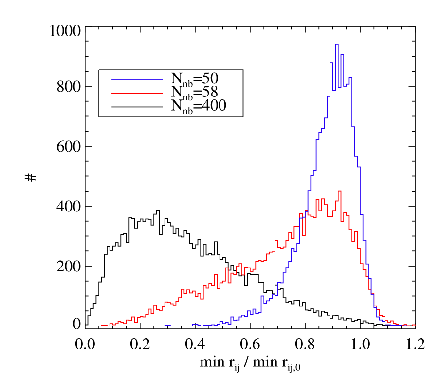
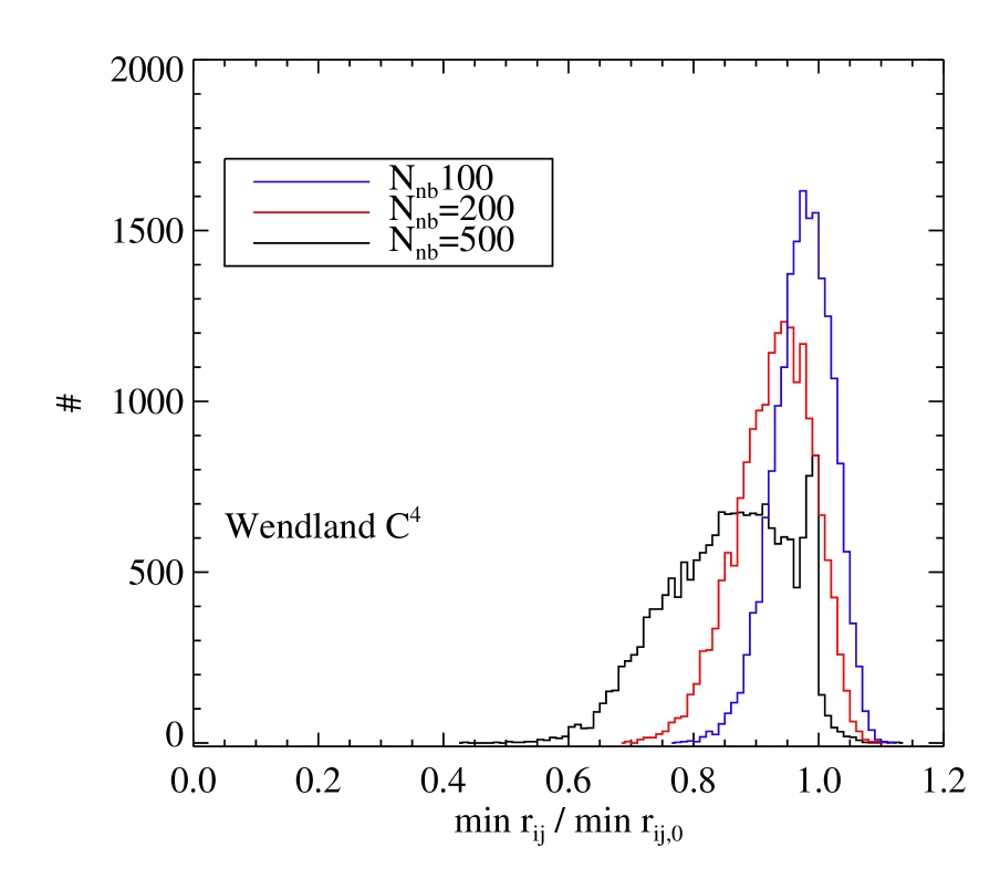
Figure 1.— Upper: The distribution of distances to the nearest neighbor $\rm{r}_{ij}$ normalized to the initial particle spacing $\rm{r}_{ij,0}$ in the Gresho vortex test at $t=1$, for the cubic spline in a portion of the simulation domain. Lower: The same histogram for a simulation with the Wendland $\rm{C^{4}}$ function. In the upper panel, once the number of neighbor exceeds a threshold, $N_{nb}=58$ for the cubic spline, close pairs of SPH particles form quickly. As a result, the volume associated with each SPH particle is not well-sampled by their neighbors. This particle clumping effectively reduces the resolution of SPH. As a comparison, this instability is not observed for the simulation with the Wendland $\rm{C^{4}}$ function.

5. Density Estimate

5.1. A set of randomly distributed points

We use a randomly distributed particle set to test the density estimate in SPH. $64^{3}$ particles are distributed randomly within a 3-D box with unit length. We use the density estimate routine in SPH with varying $N_{nb}$ from 40 to 3200 to derive the density field accordingly. In Figure 2, we plot the histogram of the density estimated at the position of each particle for varying $N_{nb}$. The variance within the density field is largest for small $N_{nb}$ values, which are shown in the red colors. As the number of neighbors increases, the distribution slowly approaches a Gaussian like distribution peaked at $\rho=1$. This behavior shows the trade-off between variance and bias in the SPH density estimate. Larger $N_{nb}$ hence larger $h$ will increasingly smear out fluctuations on short scales. However this does not show the actual accuracy of the SPH density estimate.

In fact, the precise density field in this set-up is difficult to give but the behavior of the density field can be seen from a pure statistical argument. To be more specific, the number of particles falling within a fixed volume associated with each particle follows a Poisson distribution. The expected number of such occurrences goes linearly with larger volume (larger $N_{nb}$). As a result, the standard deviation of the density distribution follows a $N_{nb}^{-0.5}$ trend. So should the trend of the standard deviation of the density distribution given by SPH if the density estimate is accurate. However, this is not strictly true as we show in the lower panel of Figure 2, where the black crosses are the measured standard deviation of the density distribution with varying $N_{nb}$. There is a significant spread that is much greater for small $N_{nb}$ than the guiding line indicating $N_{nb}^{-0.5}$. The deviation is already significant for $N_{nb}=200$, which is the recommended number by Dehnen & Aly (2012) based on a shock tube test. In the upper panel of Figure 2, we can also see there is a long tail for small $N_{nb}$ values. This suggests there is an overestimate of density where we suspect the self-contribution of each particle to the density estimates plays an exaggerated role.

In order to verity this, we carry out density estimates with self-contribution excluded for the same configuration of particles. The standard deviation of the density distribution as a function of $N_{nb}$ is shown in the red filled circles in the lower panel of Figure 2. This brings the relation much closer to the expected $N_{nb}^{-0.5}$ line where the deviation at small $N_{nb}$ is greatly reduced due to the subtraction of the self-contribution term.

Excluding the self-contribution is not the usual practice in modern SPH codes. Flebbe et al. (1994) actually advocated to use equation 3 with self-contribution excluded to give a better density calculation based on a similar comparison in 2-D. Whitworth et al. (1995) however argues that the distribution of SPH particles is essentially different from a random distribution. If particles are distributed randomly, individual particles do not care about the locations of other particles. In SPH, due to the repulsive pressure force, each SPH particle is trying to establish a zone where other SPH particles cannot easily reside. However, as we see in Figure 1, SPH forms close pairs so that the argument by Whitworth et al. (1995) is no longer valid. Note that it is not uncommon to see a value above $N_{nb}=58$ in the literature with the cubic spline. The SPH density estimate will then give a biased result for irregularly distributed particles.

This comparison actually favors the use of a large $N_{nb}$ where the distribution is highly disordered. Although the above experiment is based on a situation where the particle distribution is truly random, the realistic situation is between such a truly random distribution and a quasi-regular one. However, quasi-regular distributions are hard to achieve in multi-dimensional flows because of shear.

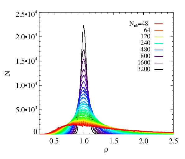
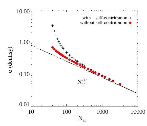
Figure 2.— Upper: The distribution of density field estimates based on an SPH smoothing routine with Wendland $C^{4}$ function on a random set of points with varying $N_{nb}$. The color scheme represents different curves with increasing $N_{nb}$ with the color from red to purple. The standard deviation decreases as we use a larger $N_{nb}$ in the SPH density estimate. For $N_{nb}>1000$, the result is close to a Gaussian peaked at $\rho=1$. Lower: The standard deviation measured in the density distribution as a function of varying $N_{nb}$. The expected trend of $\sigma\propto N^{-0.5}$ is given by the dashed-dotted line. The SPH density estimate with and without the self-contribution term is indicated by black crosses and red filled circles. Self-contribution produces an overestimate of the density where particles are randomly distributed.

5.2. A set of points in a glass configuration

A random distribution of particles, as discussed in the above section, is an extreme case for SPH simulations. We relax these particles according to the procedure described in White (1996) to allow them to evolve into a glass configuration. Given an $r^{-2}$ repulsive force, the particles settle in a equilibrium distribution which is quasi force-free and homogeneous in density. This mimics the other extreme case where SPH particles are well regulated by pressure forces. Nevertheless, the outcome of this relaxation is not perfect where tiny fluctuations in the density field are still present because of the discrete nature of the system.

We now measure the SPH density estimate on this glass configuration for different $N_{nb}$ and estimate the standard deviation of the density for each $N_{nb}$. As the upper panel in Figure 3 shows, the density distribution is much narrower than that for a random set of points. For sufficiently high $N_{nb}$, the distribution approaches a Dirac-$\delta$ distribution. The convergence is also much faster than in Figure 2. In fact, we observe a $N_{nb}^{-1}$ trend for the glass configuration. For this set up, there is no need to exclude the self-contribution term, which is consistent with Whitworth et al. (1995).

This measured $N_{nb}^{-1}$ rate is quite interesting in itself. Monaghan (1992) conjectured that the discretization error with SPH behaves as $\log(N_{nb})/N_{nb}$. This means that the randomness in the distribution of SPH particles is closer to a low discrepancy sequence rather than to a truly random one. Our experiment shows this $N_{nb}^{-1}$ (neglecting the $\log(N_{nb})$) rate is certainly appropriate for a glass configuration, which is carefully relaxed to an energy minimum state. However, this rate may not hold for a general applications.

Thus, these two examples support the dependence of the density estimate error on $N_{nb}$ as in the previous analysis. Namely, $N_{nb}^{-0.5}$ for truly random data points and $N_{nb}^{-1}$ for a distribution with good order. Realistic applications will fall between these two extremes and could be more biased towards the $N_{nb}^{-0.5}$ case.

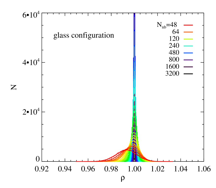
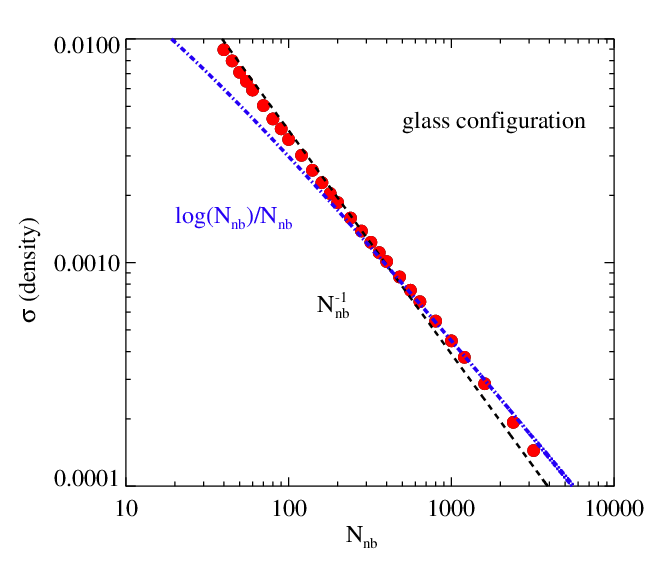
Figure 3.— Upper: Similar to Figure 2, the distribution of density field estimates based on an SPH smoothing routine with the Wendland $C^{4}$ function on a glass configuration data set for varying $N_{nb}$. The distribution of the density estimates is significantly narrower than the random point set in Figure 2. The color schemes represents different curves with increasing $N_{nb}$ for color going from red to purple. The standard deviation also decreases as we use a larger $N_{nb}$ in the SPH density estimate but at a much faster rate compared to Figure 2. Lower: The standard deviation measured in the density distributions as a function of varying $N_{nb}$. A trend of $\sigma\propto N^{-1}$ rather than $\sigma\propto N^{-0.5}$ is seen as indicated by the dashed-dotted line.

5.3. Errors in the volume estimate

We have noted that a constant scalar field is not exactly represented by the SPH method. Based on our discussion of the self-consistency of the SPH density estimation, we can further measure the magnitude of this inconsistency and its dependence on the number of neighbors $N_{nb}$. Define a parameter $Q$ as

$$Q_{a}=\sum_{j}^{N_{nb}}\frac{m_{b}}{\rho_{b}}W_{ab}(h_{a}),$$ (27)

which represents the SPH estimate of a constant scalar field $A=1$. This parameter $Q$ should follow a peaked distribution around 1 with some errors. We compute this parameter with a simple extra routine after the density calculation in the code since this parameter requires the SPH density field as input. In Figure 4, we plot the distributions of the calculated values of $Q$ for randomly distributed particles with several different $N_{nb}$ values. The distributions of $Q$ are indeed rather broad around 1. Similarly as the errors in the density estimate, the standard deviation of the distribution is consistently larger for smaller $N_{nb}$ values. Some extreme values of Q with small $N_{nb}$ are even on the order of unity. The peaks of the distribution with small $N_{nb}$ are actually slightly below 1, which indicates some bias towards a density overestimate. This is consistent with the above discussion of the self-contribution to the density overestimate at small $N_{nb}$ values.

For this random distribution of particles, increasing $N_{nb}$ will lead to a more accurate volume estimate by reducing the inconsistency in the density estimate. For example, the spread of the distribution of $Q$ for $N_{nb}=800$ is greatly reduced compared to $N_{nb}=48$. As we repeat this experiment with even more neighbors, the distribution of $Q$ approaches a Dirac-$\delta$ function eventually with the error in the volume estimate reduced to zero. In this limit, the self-consistency of SPH is finally restored. However, as in the lower panel of Figure 4, such an improvement depends slowly on the number of number $N_{nb}$ at a rate $\sigma(Q)\propto N_{nb}^{-0.5}$.

We also consider the cubic spline in this test, which is included in the lower panel of Figure 4. The dependence of Q on $N_{nb}$ for a cubic spline follows the same $N_{nb}^{-0.5}$ trend. The cubic spline shows a slightly lower magnitude for the same $N_{nb}$ compared with the Wendland $C^{4}$ function. This is because the Wendland $C^{4}$ is slightly more centrally peaked than the cubic spline. To have the same effective resolution length, a higher number of $N_{nb}$ is required for Wendland $C^{4}$ (see the table of such scaling in Dehnen & Aly (2012)). The behavior of $Q$ with respect of $N_{nb}$ is consistent with the two smoothing functions.

We then repeat this calculation with the particles in a glass configuration. The results of the Wendland $C^{4}$ function and cubic splines are presented with the solid symbols in Figure 4. As we see from the previous section, the relaxed particle distribution reduces the errors in the density estimate. The inconsistency in the volume estimate, as measured in $Q$, declines as a function of $\sigma(Q)\propto N_{nb}^{-1}$ in this case. This is true for both the Wendland $C^{4}$ function and cubic spline.

In practice, when we use SPH, the true distribution is unknown. So the error in the density estimate is difficult to quantify. We suggest a simple procedure to measure Q in simulations to give us an estimate of the overall quality of the density estimate. Based on the comparison between the $Q$ value for randomly distributed particles and particles in a glass configuration, a typical number $N_{nb}=32\ \rm{or}\ 64$ with cubic spline as often adopted in the literature leads to a volume estimate error between 1$\%$ and 10$\%$ from the true value. However, a glass configuration is a rather idealized and we suspect that SPH particles will not maintain such good order in most applications.

This error in the volume estimate, which is self-inconsistency in the SPH density estimate, also has dynamical consequences as the volume estimate,

$$d\mathbf{r}\approx\frac{m}{\rho},$$ (28)

is used for the derivation of the equations of motion. In addition to the error terms derived by Read et al. (2010), an error on the order of a percent level is already present from the density estimate step itself. The quality of the particle distribution is crucial to minimizing this error. However, once the particles deviate from a regular distribution, the errors in the equations of motion will pose another challenge for the particles to return back to an ordered configuration. One way to impose a small error in the volume estimate is to use a large $N_{nb}$. Increasing $N_{nb}$ can regulate this error with a dependence between $N_{nb}^{-0.5}$ and $N_{nb}^{-1}$.

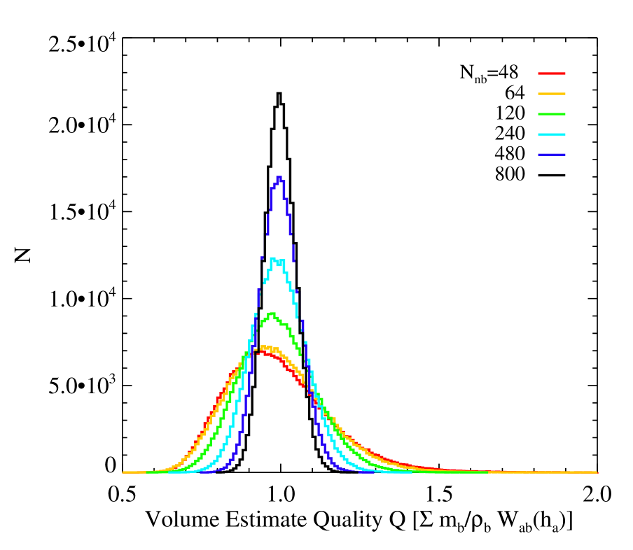
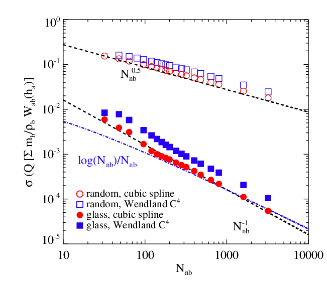
Figure 4.— . Upper: The distribution of the volume estimate quality parameter $Q_{a}=\sum m_{b}/\rho_{b}W_{ab}(h_{a})$ for the random point set used in Figure 2 for different $N_{nb}$. This quantifies the deviation from an exact partition of unity. The distribution of $Q$ slowly approaches a narrower normal distribution centered at $Q=1$ with increasing $N_{nb}$. This indicates that the volume estimate error will eventually decrease to $0$ as we have $N_{nb}\rightarrow\infty$ when the distribution of Q is essentially a Dirac-$\delta$ function at 1. Lower: The relation between $Q$ and $N_{nb}$ measured with Wendland $C^{4}$ function and with a cubic spline for the random point set and for the glass configuration respectively. For the glass configuration, the distribution of $Q$ converges to a Dirac-$\delta$ function at a rate of $N^{-1}$ for both of the smoothing functions. However, the convergence rate goes as $N^{-0.5}$ for both of the smoothing functions with the random point set.

6. Dynamical tests

In this section, we perform dynamical tests with SPH for several problems to study the convergence rates in each situation. The evolution in multi-dimensional flows is more complex than in 1-D and, as noted in §1, one-dimensional tests cannot be used to judge convergence of SPH in multi-dimensions. The test problems are chosen so analytic behaviors are known in advance (Springel (2010b); Read & Hayfield (2012); Owen (2014); Hu et al. (2014)). Also the test problems consider both smooth flows and highly turbulent flows. These test problems are purely hydro as no further compilations from other factors such as gravity are present. We also do not consider problems with shocks for our tests as the presence of discontinues will reduce the code to being at best first order accurate.

6.1. Gresho Vortex problem

The first problem is the Gresho Vortex test (Gresho & Chan, 1990). We quantify the $L_{1}$ velocity error with SPH and its convergence rate as a function of the total number of SPH particles. This test involves a differentially rotating vortex with uniform density in centrifugal balance with pressure and azimuth velocity specified according to

$$P(r)=\begin{cases}P_{0}+12.5r^{2}&(0\leq r<0.2)\\ P_{0}+12.5r^{2}+4\\ -20r+4\ln(5r)&(0.2\leq r<0.4)\\ P_{0}+2(2\ln 2-1)&(r\geq 0.4)\end{cases}$$ (29)

and

$$v_{\phi}(r)=\begin{cases}5r&(0\leq r<0.2)\\ 2-5r&(0.2\leq r<0.4)\\ 0&(r\geq 0.4).\end{cases}$$ (30)

The value of $P_{0}$ is taken to be $P_{0}=5$ following Springel (2010b) and Read & Hayfield (2012), as in the original paper of Gresho & Chan (1990). Dehnen & Aly (2012) and Hu et al. (2014) also investigate the behavior by varying this constant background pressure $P_{0}$. The velocity noise will decline for decreased $P_{0}$ such that the system is more stable. This test problem is suitable for examining the noise in the velocity field since the density field is uniform. The vortex should be time independent having the initial analytical structure.

Springel (2010b) however found that this test poses a challenge to SPH since the vortex quickly breaks up with Gadget. Dehnen & Aly (2012), Read & Hayfield (2012), and Hu et al. (2014) have tested their SPH formulation with the same problem and found improvements with a better parameterization of artificial viscosity. The convergence rate reported by Dehnen & Aly (2012) and Hu et al. (2014) is similar to the one given by Springel (2010b), $N^{-0.7}$, while Read & Hayfield (2012) give a rate of $N^{-1.4}$. This discrepancy is due to a modified version of the equations of motion by Read & Hayfield (2012). The set-up of this problem has three sharp transition points which is problematic for SPH. This test is also very sensitive to the particle noise which will can induce a false triggering of artificial viscosity.

We initialize the particles on an N$\times$N$\times$16 lattice. The number of particles vertically assures that we can extend $N_{nb}$ to several thousand for each particle without overlap. The $L_{1}$ velocity error as a function of the number of effective 1-D resolution elements $N$ is shown in Figure 5. The black squares are the simulations with $N_{nb}=120$ and the blue filled circles are the ones with $N_{nb}=200$. For the red diamonds, we run the simulation with increasing $N_{nb}$ as $N_{nb}\propto N^{3*0.4}$ starting from $N_{nb}=120$ at the lowest resolution $N=32$. The convergence rates are as $N^{-0.5}$, $N^{-0.7}$ and $N^{-1.2}$ respectively. The former two are consistent with Springel (2010b), Dehnen & Aly (2012) and Hu et al. (2014). Also, a larger number of neighbors gives a slightly faster convergence rate in this test ($N^{-0.5}$ vs. $N^{-0.7}$). For $N_{nb}=120$ and $N_{nb}=200$, the $L_{1}$ velocity error at the highest resolution at $N=500$ is actually above the convergence rate. This is what is expected based on the argument for consistency in the SPH method. A fixed $N_{nb}$ may work well for a range of different resolutions until the resolution is ultimately so high that the errors from the density estimate, from the discretized continuity equation and momentum equation, are not consistently reduced according to the corresponding resolution length $h$.

The result with varying $N_{nb}$, on the other hand, shows a much faster convergence rate as $N^{-1.2}$ with the highest resolution at $N=320$ with $N_{nb}=1900$. This validates the arguments presented earlier and shows the result given by SPH does converge to the proper solution and the convergence rate is improved in this test problem as we increase $N_{nb}$ when $h\rightarrow 0$. Such a convergence rate is actually close to the rate $p=1.4$ measured with moving mesh code Arepo (Springel, 2010a) for the same problem.

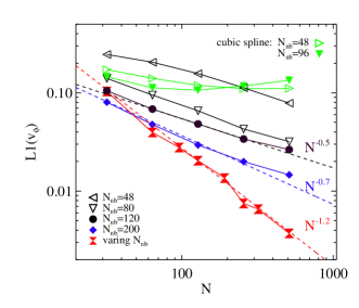
Figure 5.— . Convergence rate of the velocity field in the Gresho vortex test as a function of $N_{1D}$ with SPH. Blue filled circles are the results with a fixed number of neighbors $N_{nb}=200$ while the black filled squares are the ones with a smaller number of neighbors $N_{nb}=120$. The convergence rate shows a $N^{-0.7}$ behavior for the former and $N^{-0.5}$ for the latter. The red squares are with increased $N_{nb}$ as a function of total number of SPH particles $N$. The convergence rate for this run scales almost as $N^{-1.2}$. Such a convergence rate is close to $N^{-1.4}$ for the grid-based code in Springel (2010a).

We have also included two series of the Gresho vortex test with the cubic spline as in the green symbols in Figure 5. The performance with the cubic spline is disappointing in this test. With $N_{nb}=48$, the $L_{1}$ error reaches to a minimum value at an intermediate resolution at $N=128$. For $N_{nb}=96$, where the clumping instability is reducing the effective resolution, the minimum $L_{1}$ error is achieved at $N=64$. In terms of the absolute error, the highest resolution actually fails to give the best results. This behavior is also observed in the Gresho vortex test and the KH instability test in Springel (2010b).

6.2. Isentropic Vortex problem

This is another vortex problem described by Yee et al. (2000) and employed by Calder et al. (2002) and Springel (2011). It also has a time-invariant analytic solution. Unlike the previous test, the density and velocity profiles are both smooth. This problem will test the convergence rate of the solver for smooth flows. We generate the initial conditions in a box of size $[-5,5]^{2}$ with periodic boundary conditions. Similar to the previous test, several additional identical layers are stacked along the $z$ direction to get a thin slab configuration. The velocity field is set up as

$$v_{x}(x,y)=-y\frac{\beta}{2\pi}\exp(\frac{1-r^{2}}{2}),$$ (31)

$$v_{y}(x,y)=x\frac{\beta}{2\pi}\exp(\frac{1-r^{2}}{2}).$$ (32)

The distribution of the density field and the internal energy per unit mass are calculated according to the following temperature distribution

$$T(x,y)\equiv P/\rho=T_{\infty}-\frac{(\gamma-1)\beta^{2}}{8\gamma\pi^{2}}\exp(1-r^{2}),$$ (33)

as $\rho=T^{1/(\gamma-1)}$ and $u=T/(\gamma-1)$. Consequently, the entropy $P/\rho^{\gamma}$ is a constant within the domain. As in Springel (2011), we then measure the $L_{2}$ error in the density field at $t=8.0$ obtained with our code with respect to the analytical density field for different resolutions. The result if shown in Figure 6 where the blue filled circles are obtained with $N_{nb}=200$ while the red diamonds are with varying $N_{nb}$. The dashed line is a $N^{-2}$ trend with the dashed-dotted line taken from Springel (2011) measured with the Arepo code.

The overall magnitude of the error with SPH is also close to the one for the Arepo simulation in Springel (2011). In fact, the result for $N_{nb}=200$ with SPH shows a second order convergence for the first four resolutions, but for the two highest resolution runs the $L_{2}$ density error starts to reach a plateau. Beginning with $N_{nb}=200$ at $N=256$, we re-simulate the two high resolution runs with $N_{nb}\propto N^{3*0.5}$. As a result, the overall error is reduced and is now consistent with the expected rate of $N^{-2}$.

The above result based on the isentropic vortex problem shows that SPH can be a second-order accurate scheme as long as the other errors do not dominate over the “smoothing error” introduced from the density estimate. Again, the condition $N\rightarrow\infty,h\rightarrow 0\$ and $\ N_{nb}\rightarrow\infty$ needs to be satisfied. As for the fixed $N_{nb}$ run, starting from $N=512$ the other errors rather than the “smoothing error” become dominant and start to degrade the performance of SPH.

In order to see the effects of the discretization error, we have repeated this experiment with smaller $N_{nb}$ and also using the cubic spline. For the two series of $N_{nb}=80$ and $N_{nb}=48$, as in green symbols in Figure 6, the convergence rate systematically slows down from $N^{-1.7}$ to $N^{-1.3}$ from a second order convergence rate. The convergence rate with the cubic spine, where $N_{nb}=48$, is the slowest one. Moreover, it shows signs of turning over at the highest resolution with the cubic spline.

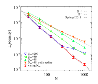
Figure 6.— . Convergence rate of the isentropic vortex test as a function of $N_{1D}$ with SPH code. The error is computed from the $L_{2}$ norm of the density field at $t=8.0$ when the vortex has completed a full rotation. Blue filled circles are the result for a fixed number of neighbors $N_{nb}=200$. The convergence rate exhibits a $N^{-2}$ behavior except for the two high resolution runs. The red filled diamonds are the two high resolution runs for increasing $N_{nb}$ and now the error is consistent with the expected $N^{-2}$ trend.

6.3. Subsonic turbulence

In this section, we move to a more complex problem involving the chaotic feature of multi-dimensional flows with SPH. In particular, we simulate subsonic turbulence in the gas (which is weakly compressible). Following Bauer & Springel (2012) and Price (2012a), we employ a periodic box with unit length filled with an isothermal gas $\gamma=1$ with unit mean gas density and unit sound speed. The initial positions of the particles are set on a cubic lattice. The stirring force field is set up in Fourier space and we only inject energy between k = 6.28 and k = 12.56. The amplitude of these modes follows a -5/3 law as: $P(k)\propto k^{-5/3}$, while the phases are calculated for an Ornstein$-$Uhlenbeck process

$$x_{t}=fx_{t-\Delta t}+\sigma\sqrt{(1-f^{2})}Z_{n},$$

such that a smoothly varying driving field with finite correlation time is obtained. The parameters in the Ornstein$-$Uhlenbeck process are identical to the ones adopted by Bauer & Springel (2012) and Price (2012a) as well as Hopkins (2013). A Helmholtz decomposition in k-space is applied before the Fourier transformation to yield a pure solenoidal component in the driving force field. At every time step, before the hydro force calculation, this driving routine is called to compute the acceleration. The magnitude of the driving force is adjusted such that the $r.m.s.$ velocity is at $\sim 0.2c_{s}$ once the system reaches a quasi-equilibrium state. Besides the routine to calculate the driving force, we have also included a function to measure the velocity power spectrum on the fly. The turbulent velocity power spectrum is calculated whenever a new snapshot is written. We use the “nearest neighbor sampling” method for our estimate. Finally the 1D power spectrum is obtained by averaging the velocity power with each component in fixed $|\mathbf{k}|$ bins. We use the time-averaged velocity power spectra between $t=10$ and $t=20$ for the following comparison.

We emphasize that our SPH code is able to give improved performance in this test over the previous studies of Bauer & Springel (2012) and Price (2012b). A snapshot of the velocity field is shown in Figure 7 in a high resolution test with $256^{3}$ particles. Our SPH code is able to resolve finer structures compared to the other two studies noted. The velocity field is qualitatively closer to the one simulated with grid based codes. This is a result of the use of the artificial viscosity switch proposed by Cullen & Dehnen (2010) and the Wendland $C^{4}$ smoothing kernel.

Four different resolutions, $64^{3}$, $80^{3}$, $96^{3}$ and $128^{3}$, are used for a resolution study. We actually fix the smoothing length $h$ for all the simulations based on $N_{nb}=200$ for the $64^{3}$ resolution run and subsequently scale $N_{nb}$ for the other three cases. This is done to directly test the effect of varying $N_{nb}$ on the hydrodynamics by controlling the same resolution length $h$ so that the smoothing error is fixed. The projected velocity maps of these four resolutions are shown in Figure 8. The velocity fields are similar to one another between these four simulations.

In Figure 9, we compare the velocity power spectrum for these four resolutions. We multiply the power spectrum by $k^{5/3}$ so that the inertial range described by $P(k)\propto k^{-5/3}$ shows up as a horizontal line. The power spectrum shows good agreement with the $k^{-5/3}$ law on large scales. The velocity power goes down significantly below that once the wave number $k$ is above 40. However, there is significant power contained on the smallest scales. The spatial extent where neighbor particles are searched corresponds to $k\sim 110$, which is the range where the turn-over is observed. This turn-over can be seen as the result of dissipation of velocity noise on the resolution scale (Hopkins, 2013).

Improvements with varying $N_{nb}$ in this test problems can be seen. The effect of varying $N_{nb}$ on the velocity power spectrum is visible on both large and small scales. With more neighbors, the velocity field on the kernel scale (smoothing length $h$) is better regulated as the power is reduced by an order of magnitude. This can be also seen in that the turn-over point for higher resolution increasingly shifts to a higher $k$ value. On large scales where the modes are well resolved, more neighbors also help to bring the power spectrum into better agreement with the $k^{-5/3}$ law. This can be verified by comparing the red and purple lines for $128^{3}$ and $64^{3}$ in Figure 9. The variance on the power spectrum between $k=10$ and $k=30$ is reduced for the latter case. The velocity power contained within $k=30$ and $k\sim 110$ is also significantly higher in the $128^{3}$ run with $N_{nb}=1600$ than $64^{3}$ with $N_{nb}=200$. The result is that there is increasingly less power in the noisy motion on the kernel scale but more power in a coherent fashion. The conclusion is that $N_{nb}$ does play an important role in this subsonic turbulence test as suggested by Bauer & Springel (2012). This also agrees with the consistency requirement for SPH in order to recover the continuous limit that the “discretization errors” also need to be reduced with $h\rightarrow 0$.

Figure 10 shows the value of $Q$, as defined above, in the turbulence tests at $t=15$. We have also over-plotted the trend of Q from the static distribution of random particles and the glass configuration in the previous section. This allows us to use $Q$, which describes the deviation from an exact partition of unity, to access the degree of disorder in realistic applications of SPH. In fact, the distribution of $Q$ for these six snapshots are between the two static cases. The trend of $Q$ with respect to $N_{nb}$, however, is quite shallow among these dynamical cases, indicating a $N_{nb}^{-0.5}$ trend. SPH is not able to re-order the particles to a distribution with the degree of order characterized by the glass configuration. The degree of disorder could be much higher in post-shock flows frequently encountered in astrophysical simulations than what we have found in these weakly compressible turbulence flows with SPH since the density variation is much higher in the former.

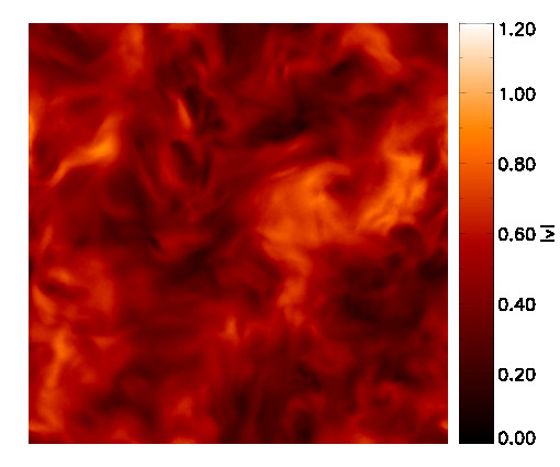
Figure 7.— . A high resolution subsonic turbulence test with $256^{3}$ particles showing the magnitude of the velocity field at $t=10.0$ for a thin slice in the box. A cross comparison between this figure and the ones in Bauer & Springel (2012) and Price (2012b) at the same resolution shows that our SPH code is able to resolve the finest structures among all three. The velocity field is qualitatively closer to the one simulated with a grid based code. This is a result of the use of the artificial viscosity switch proposed by Cullen & Dehnen (2010) and the Wendland $C^{4}$ smoothing kernel. $N_{nb}=200$ is used in this example.

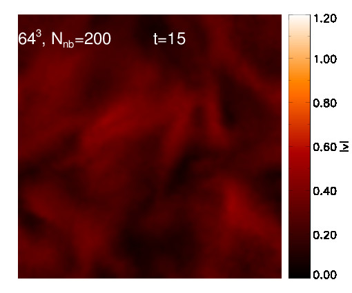
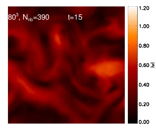
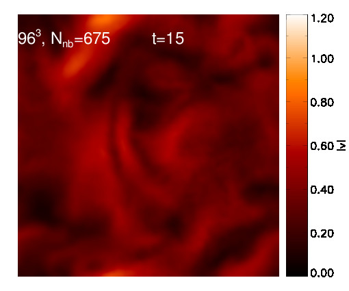
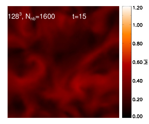
Figure 8.— Projected maps of velocity field for four subsonic turbulence tests. The total number of SPH particles is increased from $64^{3}$ to $128^{3}$ while the number of number of neighbors $N_{nb}$ is also increased accordingly in order to have the same smoothing length $h$ for all the simulations.

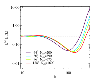
Figure 9.— The velocity power spectrum in a driven subsonic turbulence test at different resolutions. The velocity power is multiplied by $k^{5/3}$, where $k$ is the wave number, such that the inertial range will show up as a horizontal line. Different total numbers of SPH particles are used while the number of neighbors are set up such that the “smoothing length” $h$ is the same for all the simulations. Even with the same nominal “h-resolution”, the $128^{3}$ run shows an improvement over the $64^{3}$ run, especially for the location of the point of turn-over from the minimum on small scales and the increased velocity power on large scales.

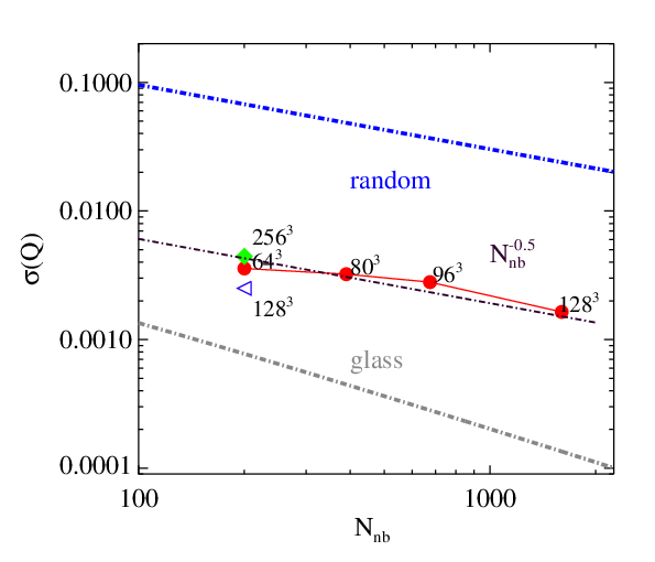
Figure 10.— The distribution of $Q=\sum m_{b}/\rho_{b}Wij(h_{a})$ for several snapshots at the same $t$ in the subsonic turbulence tests in order to access the degree of disorder in realistic SPH applications. The trend of Q from the static random particles and the glass configuration are also over-plotted here. The distribution of $Q$ for these six snapshots is between the two static cases. The trend of $Q$ with respect to $N_{nb}$, however, is quite shallow in these dynamical cases. These points roughly follow a $N_{nb}^{-0.5}$ trend. SPH is not able to reorder the particles to a distribution with the degree of order characterized by a glass configuration.

7. Conclusions

The main findings of our study are as follows:

• We argue that the requirements of consistency and self-consistency within the SPH framework require that $N\rightarrow\infty,h\rightarrow 0$ and $N_{nb}\rightarrow\infty$ need to be satisfied to obtain the true continuum behavior of a flow. We summarize the errors from the smoothing step and from the discretization step in the SPH density estimate and propose a power-law scaling between the desired $N_{nb}$ given the total number of SPH particles $N$ in order to have a consistent and convergent scheme. The dependence $N_{nb}\propto[N^{0.40},N^{0.57}]$ is derived based on a balance between these two types of errors for commonly used smoothing kernels.

• We verify the error dependence on $N_{nb}$ for the discretization error with a quasi-ordered glass configuration and a truly random one. The range for the power-law index between $N_{nb}$ and $N$ is obtained based on these two extreme conditions. The discretization error in the density estimate decreases roughly as $\log({N_{nb}})/N_{nb}$ for the glass configuration and as $N_{nb}^{-0.5}$ for the random distribution.

• We propose a simple method to calculate a parameter $Q$, which measures the deviation from an exact partition of unity in SPH. The error in the volume estimate in SPH is further examined for a glass configuration and a random one. In agreement with the behavior of the density estimate error, this quantity also shows the same dependence on $N_{nb}$ in these two situations. In realistic applications, the error introduced with the density estimate step itself is on the order of several percent for the $N_{nb}$ value used in most published work.

• We use the Wendland $C^{4}$ function as a new smoothing kernel to perform dynamical tests with a varying $N_{nb}$ to avoid the clumping instability. We confirm that particle pairs do not form even with a large value of $N_{nb}$. The artificial viscosity by Cullen & Dehnen (2010) also greatly improves the performance of our SPH code. As a consequence, the results from our study are not influenced by the numerical artifacts from these two aspects as in some of the previous studies.

• A fixed $N_{nb}$, which indicates an inconsistent scheme, gives a slow convergence rate as reported by previous studies in the two vortex problems. As shown in the figures, the convergence rate levels off and eventually turns over for sufficiently fine resolution. Also the error obtained with the cubic spline is larger than for the Wendland $C^{4}$ function. The cubic spline actually exaggerates the discretization error as the Wendland $C^{4}$ function is much smoother.

• For smooth flows, as seen in the isentropic vortex problem, varying $N_{nb}$ according to the proposed power-law dependence can give second-order convergence. The same improvement is seen in the Gresho vortex test, where several discontinuities are included. The convergence rate $p=1.2$ with varying $N_{nb}$ is closer to the rate $p=1.4$ measured with the second-order accurate moving mesh Arepo code for the same problem.

• For highly turbulent flows, the velocity noise poses another challenge in addition to the errors in the density estimate for the SPH particles to retain an ordered configuration. Though our code is able to give a better result in the subsonic turbulence test compared with previous studies, the velocity noise on the kernel scale is always present. This velocity noise can be reduced by an order of magnitude with a larger $N_{nb}$, but the inertial range resolved with SPH code only shows a slight improvement.

• We measure the randomness of SPH particles in the above subsonic turbulence tests using the calculation of $Q$. This further verifies our assumptions when deriving the dependence of $N_{nb}$ on $N$. The distribution of SPH particles in this example is indeed between a truly random configuration and a quasi-ordered case. This approach can be used in general to quantify the randomness in SPH in applications. Unfortunately, SPH is not able to rearrange the particles into a highly ordered configuration characterized by a low discrepancy sequence.

• The usual practice of using a fixed $N_{nb}$ indicates that the same level of noise will be present even if higher resolution is used. This error can be stated as a “zeroth order” term which is independent of resolution. Moreover, the errors introduced can be roughly approximated by a Gaussian distribution around the true value provided $N_{nb}$ is large enough so that the self-contribution term is not significant even for highly random distributions.

We emphasize that the inconsistency and the errors associated with particle disorder is not a specific feature to a particular SPH code but is rather a generic problem. In fact, the set of equations in Gadget are fully conservative since they are derived from the Euler-Lagrange equations (see Springel & Hernquist 2002, Springel 2010b and Price 2012b). To our knowledge, this approach has not been fully adopted by the community yet. The conservation of mass, linear momentum, angular momentum and total energy has been long recognized to be the unique advantage over other techniques. Indeed, its conservative nature, its robustness and its simple form have made it a popular tool for astrophysical modeling and in other disciplines. However, the errors associated with the finite summation $error_{d}$, usually termed as “noise” in the SPH literature, and its impact on the convergence of SPH has not been well understood so far. As we discussed earlier, such an error naturally and inevitably emerges from the density estimate itself and also from the momentum equation when evolving the system.

Obviously, one promising direction to improve the particle method is to use a more accurate volume estimate. It is possible to derive a numerical scheme which can reproduce a polynomial up to the $n^{th}$ order polynomial exactly following the procedure by Liu & Liu (2006). In practice, it is sufficient to eliminate the zero-th order error by renormalization such that the corrected scheme is second-order accurate by symmetry.

Recently, Hopkins (2014) proposed a new class of gridless Lagrangian methods which use finite-element Godunov schemes. These gridless methods dramatically reduce the low-order errors and numerical viscosity in SPH method and significantly improve accuracy and convergence. They show better performance in resolving fluid-mixing instabilities, shocks and subsonic turbulence, which is critical in a wide range of physical and astrophysical problems.

We caution against equating numerical precision with physical accuracy of a simulation because both physics and numerics play roles in the modeling of a complex system. For example, we compared cosmological hydrodynamical simulations of a Milky-Way like galaxy using both the improved Gadget code (presented in this paper) and the gridless GIZMO code by Hopkins (2014) with the same initial conditions, physics prescriptions and resolutions, and found that both simulations produced similar galaxy properties such as disk mass, size and kinematics, although GIZMO resolves the spiral structures better. These results suggest that the robustness of astrophysical simulations depends not only on the numerical algorithms, but also on the physical processes, as highlighted also in a number of recent papers on galaxy simulations (e.g., Scannapieco et al. 2012; Hopkins et al. 2014; Vogelsberger et al. 2013, 2014a, 2014b; Schaye et al. 2014).

References

- Agertz et al. (2007) Agertz, O., Moore, B., Stadel, J., Potter, D., Miniati, F., Read, J., Mayer, L., Gawryszczak, A., Kravtsov, A., Nordlund, Å., Pearce, F., Quilis, V., Rudd, D., Springel, V., Stone, J., Tasker, E., Teyssier, R., Wadsley, J., & Walder, R. 2007, MNRAS, 380, 963
- Bauer & Springel (2012) Bauer, A., & Springel, V. 2012, MNRAS, 423, 2558
- Calder et al. (2002) Calder, A. C., Fryxell, B., Plewa, T., Rosner, R., Dursi, L. J., Weirs, V. G., Dupont, T., Robey, H. F., Kane, J. O., Remington, B. A., Drake, R. P., Dimonte, G., Zingale, M., Timmes, F. X., Olson, K., Ricker, P., MacNeice, P., & Tufo, H. M. 2002, ApJS, 143, 201
- Cullen & Dehnen (2010) Cullen, L., & Dehnen, W. 2010, MNRAS, 408, 669
- Dehnen & Aly (2012) Dehnen, W., & Aly, H. 2012, MNRAS, 425, 1068
- Durier & Dalla Vecchia (2012) Durier, F., & Dalla Vecchia, C. 2012, MNRAS, 419, 465
- Flebbe et al. (1994) Flebbe, O., Muenzel, S., Herold, H., Riffert, H., & Ruder, H. 1994, ApJ, 431, 754
- García-Senz et al. (2014) García-Senz, D., Cabezón, R. M., Escartín, J. A., & Ebinger, K. 2014, A&A, 570, A14
- Genel et al. (2013) Genel, S., Vogelsberger, M., Nelson, D., Sijacki, D., Springel, V., & Hernquist, L. 2013, MNRAS, 435, 1426
- Gingold & Monaghan (1977) Gingold, R. A., & Monaghan, J. J. 1977, MNRAS, 181, 375
- Gresho & Chan (1990) Gresho, P. M., & Chan, S. T. 1990, International Journal for Numerical Methods in Fluids, 11, 621
- Hayward et al. (2014) Hayward, C. C., Torrey, P., Springel, V., Hernquist, L., & Vogelsberger, M. 2014, MNRAS, 442, 1992
- Hernquist (1993) Hernquist, L. 1993, ApJ, 404, 717
- Hernquist & Katz (1989) Hernquist, L., & Katz, N. 1989, ApJS, 70, 419
- Hopkins (2013) Hopkins, P. F. 2013, MNRAS, 428, 2840
- Hopkins (2014) —. 2014, ArXiv e-prints:1409.7395
- Hopkins et al. (2014) Hopkins, P. F., Kereš, D., Oñorbe, J., Faucher-Giguère, C.-A., Quataert, E., Murray, N., & Bullock, J. S. 2014, MNRAS, 445, 581
- Hu et al. (2014) Hu, C.-Y., Naab, T., Walch, S., Moster, B. P., & Oser, L. 2014, MNRAS, 443, 1173
- Kawata et al. (2013) Kawata, D., Okamoto, T., Gibson, B. K., Barnes, D. J., & Cen, R. 2013, MNRAS, 428, 1968
- Liu & Liu (2006) Liu, M. B., & Liu, G. R. 2006, Appl. Numer. Math., 56, 19
- Lucy (1977) Lucy, L. B. 1977, AJ, 82, 1013
- Monaghan (1985) Monaghan, J. 1985, Journal of Computational Physics, 60, 253
- Monaghan (1992) Monaghan, J. J. 1992, ARA&A, 30, 543
- Monaghan (2005) —. 2005, Reports on Progress in Physics, 68, 1703
- Owen (2014) Owen, M. 2014, International Journal for Numerical Methods in Fluids, 75, 749
- Price (2008) Price, D. J. 2008, Journal of Computational Physics, 227, 10040
- Price (2012a) —. 2012a, MNRAS, 420, L33
- Price (2012b) —. 2012b, Journal of Computational Physics, 231, 759
- Quinlan et al. (2006) Quinlan, N. J., Basa, M., & Lastiwka, M. 2006, International Journal for Numerical Methods in Engineering, 66, 2064
- Read & Hayfield (2012) Read, J. I., & Hayfield, T. 2012, MNRAS, 422, 3037
- Read et al. (2010) Read, J. I., Hayfield, T., & Agertz, O. 2010, MNRAS, 405, 1513
- Robinson & Monaghan (2012) Robinson, M., & Monaghan, J. J. 2012, International Journal for Numerical Methods in Fluids, 70, 37
- Saitoh & Makino (2009) Saitoh, T. R., & Makino, J. 2009, ApJ, 697, L99
- Saitoh & Makino (2013) —. 2013, ApJ, 768, 44
- Scannapieco et al. (2012) Scannapieco, C., Wadepuhl, M., Parry, O. H., Navarro, J. F., Jenkins, A., Springel, V., Teyssier, R., Carlson, E., Couchman, H. M. P., Crain, R. A., Dalla Vecchia, C., Frenk, C. S., Kobayashi, C., Monaco, P., Murante, G., Okamoto, T., Quinn, T., Schaye, J., Stinson, G. S., Theuns, T., Wadsley, J., White, S. D. M., & Woods, R. 2012, MNRAS, 423, 1726
- Schaye et al. (2014) Schaye, J., Crain, R. A., Bower, R. G., Furlong, M., Schaller, M., Theuns, T., Dalla Vecchia, C., Frenk, C. S., McCarthy, I. G., Helly, J. C., Jenkins, A., Rosas-Guevara, Y. M., White, S. D. M., Baes, M., Booth, C. M., Camps, P., Navarro, J. F., Qu, Y., Rahmati, A., Sawala, T., Thomas, P. A., & Trayford, J. 2014, ArXiv e-prints:1407.7040
- Schuessler & Schmitt (1981) Schuessler, I., & Schmitt, D. 1981, A&A, 97, 373
- Springel (2005) Springel, V. 2005, MNRAS, 364, 1105
- Springel (2010a) —. 2010a, MNRAS, 401, 791
- Springel (2010b) —. 2010b, ARA&A, 48, 391
- Springel (2011) —. 2011, ArXiv e-prints:1109.2218
- Springel & Hernquist (2002) Springel, V., & Hernquist, L. 2002, MNRAS, 333, 649
- Vogelsberger et al. (2013) Vogelsberger, M., Genel, S., Sijacki, D., Torrey, P., Springel, V., & Hernquist, L. 2013, MNRAS, 436, 3031
- Vogelsberger et al. (2014a) Vogelsberger, M., Genel, S., Springel, V., Torrey, P., Sijacki, D., Xu, D., Snyder, G., Bird, S., Nelson, D., & Hernquist, L. 2014a, Nature, 509, 177
- Vogelsberger et al. (2014b) Vogelsberger, M., Genel, S., Springel, V., Torrey, P., Sijacki, D., Xu, D., Snyder, G., Nelson, D., & Hernquist, L. 2014b, MNRAS, 444, 1518
- Vogelsberger et al. (2012) Vogelsberger, M., Sijacki, D., Kereš, D., Springel, V., & Hernquist, L. 2012, MNRAS, 425, 3024
- White (1996) White, S. D. M. 1996, in Cosmology and Large Scale Structure, ed. R. Schaeffer, J. Silk, M. Spiro, & J. Zinn-Justin, 349
- Whitworth et al. (1995) Whitworth, A. P., Bhattal, A. S., Turner, J. A., & Watkins, S. J. 1995, A&A, 301, 929
- Wozniakowski (1991) Wozniakowski, H. 1991, Bulletin (New Series) of the American Mathematical Society, 24, 185
- Yee et al. (2000) Yee, H., Vinokur, M., & Djomehri, M. 2000, Journal of Computational Physics, 162, 33