Verification of exceptional points in the collapse dynamics of Bose-Einstein condensates

Abstract

In Bose-Einstein condensates with an attractive contact interaction the stable ground state and an unstable excited state emerge in a tangent bifurcation at a critical value of the scattering length. At the bifurcation point both the energies and the wave functions of the two states coalesce, which is the characteristic of an exceptional point. In numerical simulations signatures of the exceptional point can be observed by encircling the bifurcation point in the complex extended space of the scattering length, however, this method cannot be applied in an experiment. Here we show in which way the exceptional point effects the collapse dynamics of the Bose-Einstein condensate. The harmonic inversion analysis of the time signal given as the spatial extension of the collapsing condensate wave function can provide clear evidence for the existence of an exceptional point. This method can be used for an experimental verification of exceptional points in Bose-Einstein condensates.

I Introduction

In Bose-Einstein condensates with attractive interactions stationary solutions to the Gross-Pitaevskii equation exist only in certain regions of the parameter space governing the physics of the condensates. For the case of an attractive s-wave contact interaction the condensate collapses when, for given negative scattering length, the number of particles becomes too large Dalfovo and Stringari (1996); Pérez-García et al. (1997). Alternatively, the collapse can be induced experimentally by tuning the scattering length in the vicinity of Feshbach resonances by adjusting an external magnetic field Donley et al. (2001). The critical parameter values where collapse occurs correspond to solutions to the stationary Gross-Pitaevskii equation, where the stable ground state and an unstable excited state emerge in a tangent bifurcation Huepe et al. (1999, 2003). The coalescence of two or even more eigenstates at critical points in the parameter space, where both the eigenvalues and the eigenvectors of the states pass through a branch point singularity and become identical, is a characteristic property of an “exceptional point” Kato (1966); Moiseyev (2011).

Exceptional points cannot occur in quantum systems described by the linear Schrödinger equation with Hermitian operators. However, they can appear in systems described by non-Hermitian matrices or in nonlinear systems which depend on a multidimensional parameter space. Examples are discussed, e.g., for complex atoms in laser fields Latinne et al. (1995), a double $\delta$ well Korsch and Mossmann (2003), the scattering of a beam of particles by a double barrier potential Hernández et al. (2006), non-Hermitian Bose-Hubbard models Graefe et al. (2008), or models used in nuclear physics von Brentano and Philipp (1999). The resonant behavior of atom waves in optical lattices Oberthaler et al. (1996) also shows structures originating from exceptional points. However, the phenomenon of exceptional points in physics is not restricted to quantum mechanics. Acoustic modes in absorptive media Shuvalov and Scott (2000) represent a mechanical system in which branch-point singularities appear. Furthermore, manifestations of exceptional points can be seen in optical devices Berry (1994); Klaiman et al. (2008); Wiersig et al. (2008). The most detailed experimental analysis of exceptional points has been carried out for the resonances of microwave cavities Philipp et al. (2000); Dembowski et al. (2003); Dietz et al. (2007), which open the possibility of studying the properties of the complex resonance frequencies and the wave functions.

Critical phenomena also occur in nonlinear systems. Various types of bifurcations which are classified in catastrophe theory Poston and Stewart (1978) are branch point singularities and resemble exceptional points in many aspects. Bose-Einstein condensates are described in a mean-field approach by the nonlinear Gross-Pitaevskii equation. The stationary solutions of this equation exhibit a coalescence of two states due to the nonlinearity of the equation, which turns out to be a branch-point singularity of the energy eigenvalues and wave functions Cartarius et al. (2008a); Rapedius and Korsch (2009). There is only one linearly independent eigenvector of the coalescing states at the exceptional point. These systems exhibit the typical consequences of exceptional points, viz. the permutation of eigenstates when an exceptional point is encircled in the parameter space and a special type of geometric phase.

For condensates with an attractive gravity-like $1/r$ interaction O’Dell et al. (2000); Cartarius et al. (2008a, b) and for dipolar condensates Griesmaier et al. (2005); Koch et al. (2008); Lahaye et al. (2008, 2009); Köberle et al. (2009); Gutöhrlein et al. (2013) the bifurcation points of the ground and excited state have been analyzed in theoretical computations to verify that they show signatures of exceptional points. To that aim the stationary states of the nonlinear system can be approximated by a linear matrix model with a non-Hermitian matrix. However, the dynamics cannot be described by a linear model because the superposition principle is not valid in nonlinear systems, i.e., there is no unitary time evolution of the condensate wave function.

The stability properties of Bose-Einstein condensates are determined by the eigenvalues of the Bogoliubov-de Gennes equations which are obtained by linearization of the Gross-Pitaevskii equation around the stationary states. The existence of complex frequencies in the Bogoliubov spectrum indicates a dynamical instability of the condensate Skryabin (2000); Kawaguchi and Ohmi (2004); Kreibich et al. (2012, 2013). Typically a stable and an unstable state are created in a tangent bifurcation, and a state changes its stability properties when running through an exceptional point at a pitchfork bifurcation. However, there are counterexamples where the occurrence of an exceptional point and the stability change do not match. A discrepancy between the occurrence of a pitchfork bifurcation and the stability change has been observed in $\mathcal{P}T$-symmetric states of a condensate where atoms are incoupled to one side and extracted from the other Haag et al. (2014); Löhle et al. (2014).

An important property of exceptional points, which follows from the branch point singularity structure, is the permutation of the eigenvalues if the exceptional point is encircled in the parameter space Kato (1966). Using an analytic continuation of the Gross-Pitaevskii equation the bifurcation points in Bose-Einstein condensates can be encircled in the complex plane of the scattering length. Indeed, after one circle around the critical point a permutation of the two states is present clearly indicating the existence of an exceptional point Cartarius et al. (2008a); Köberle et al. (2009); Gutöhrlein et al. (2013). However, complex scattering lengths within the analytically continued Gross-Pitaevskii equation are not experimentally accessible, and thus the method mentioned above cannot be used for an experimental verification of exceptional points in Bose-Einstein condensates. The aim of this Paper is to present an alternative method for the verification of the exceptional points. It is based on dynamical properties of the condensates and can also be applied in an experiment.

While the investigations of exceptional points mentioned above are related to non-Hermitian time-independent Hamiltonians effects of exceptional points also occur in time-dependent systems Latinne et al. (1995); Stehmann et al. (2004); Cartarius and Moiseyev (2011); Uzdin et al. (2013). Uzdin et al. Uzdin et al. (2013) have shown that a sharp transition from an oscillatory to a monotonic exponential dynamics occurs in the time evolution of a single particle in a harmonic trap with a certain time-dependent frequency $\omega(t)$, and that this transition corresponds to an exceptional point. The time evolution of the particle can be analyzed with the harmonic inversion method as shown in Fuchs et al. (2014). Here an exceptional point is characterized by the degeneracy of two or more frequencies in the frequency spectrum of the time signal.

The dynamics of a Bose-Einstein condensate described by the nonlinear time-dependent Gross-Pitaevskii equation differs fundamentally from the dynamics of a linear quantum system. Nonetheless, we will show that the existence of exceptional points can be verified in the dynamics of the condensate when the harmonic inversion analysis is applied to a restricted region of the time evolution. Starting with a condensate in the stable region of the parameter space the scattering length can be decreased and then the spatial extension of the condensate wave function is observed as a function of time. At the critical scattering length the time signal of the collapsing condensate exhibits characteristic features in a local time domain which indicates an exceptional point.

The paper is organized as follows. The dynamics of Bose-Einstein condensates using a variational approach to the condensate wave function is discussed in Sec. II. In Sec. III we show that signatures of exceptional points can be obtained by a local harmonic inversion analysis of time signals. The results are presented in Sec. IV and conclusions are drawn in Sec. V.

II Variational approach to the condensate dynamics

In this Paper we investigate Bose-Einstein condensates with an s-wave contact interaction between particles with mass $m$ in a spherically symmetric harmonic trap with frequency $\omega$. With the particle number $N$, the scattering length $a$, and the units $\ell_{\rm u}=\sqrt{\hbar/(m\omega)}$ for length, $m_{\rm u}=2m$ for mass, $E_{\rm u}=\hbar\omega/2$ for energy, and $t_{\rm u}=2/\omega$ for time the dynamics of the condensate wave function is described in a mean-field approach by the time-dependent Gross-Pitaevskii equation Pitaevskii and Stringari (2003),

$$\mathrm{i}\frac{\mathrm{d}}{\mathrm{d}t}\psi(\bm{r},t)=\left[-\Delta+r^{2}+8\pi Na|\psi(\bm{r},t)|^{2}\right]\psi(\bm{r},t)\;.$$ (1)

For the wave function we use an ansatz given as superposition of $N_{g}$ Gaussian functions,

$$\psi(\bm{r},t)=\sum_{k=1}^{N_{g}}\exp(-A_{k}r^{2}-B_{k})\equiv\sum_{k=1}^{N_{g}}g_{k}\;,$$ (2)

where the $A_{k}$ and $B_{k}$ are time-dependent complex variational parameters. Variational approaches with coupled Gaussian functions have already been established in a large variety of applications as a powerful tool for numerical computations of Bose-Einstein condensates Cartarius et al. (2008b); Rau et al. (2010a, b, c); Eichler et al. (2011); Marquardt et al. (2012); Gutöhrlein et al. (2013). Equations of motion for the variational parameters $A_{k}$ and $B_{k}$ are obtained with the time-dependent variational principle McLachlan (1964), and read

$$\dot{A}_{k} =-4\mathrm{i}A_{k}^{2}+\mathrm{i}V_{2,k}\;,$$ (3a)

$$\dot{B}_{k} =6\mathrm{i}A_{k}+\mathrm{i}V_{0,k}\;,$$ (3b)

for $k=1,\dotsc,N_{g}$. The parameters $V_{0,k}$ and $V_{2,k}$ in Eq. (3) are solutions of the linear set of equations (for $l=1,\dotsc,N_{g}$)

$$\sum_{k=1}^{N_{g}}\left(\begin{array}[]{cc}\braket{g_{l}}{g_{k}}&\braket{g_{l}}{r^{2}}{g_{k}}\\[3.0pt] \braket{g_{l}}{r^{2}}{g_{k}}&\braket{g_{l}}{r^{4}}{g_{k}}\end{array}\right)\cdot\left(\begin{array}[]{c}V_{0,k}\\[3.0pt] V_{2,k}\end{array}\right)$$ (8)

$$= \sum_{k=1}^{N_{g}}\left(\begin{array}[]{c}\braket{g_{l}}{r^{2}+8\pi Na}{\psi|^{2}|g_{k}}\\[3.0pt] \braket{g_{l}}{r^{4}+8\pi Nar^{2}}{\psi|^{2}|g_{k}}\end{array}\right)\,.$$ (11)

All integrals with the Gaussian functions $g_{k}$ in Eq. (11) can be solved analytically and are listed in the Appendix. For more details of the variational approach and derivations see Rau et al. (2010b).

The stationary states of the condensates are obtained by a numerical root search as fixed points of the equations of motion (3) with the normalization condition $\langle\psi|\psi\rangle=1$. The mean-field energy of the ground and excited state computed with $N_{g}=1$ to $4$ coupled Gaussian functions is presented in Fig. 1. As can be seen the mean-field energy converges rapidly with increasing number of Gaussian functions, and the results obtained with three or more Gaussian functions fully agree with numerically exact simulations. The ground and excited state emerge in a tangent bifurcation at a critical value $(Na)_{\rm cr}$ of the scattering length which depends on the number of Gaussians $N_{g}$ used in the computation. The numerical values of $(Na)_{\rm cr}$ are given in Table 1. Like the mean-field energy the critical scattering length converges rapidly with increasing number of Gaussian functions used in the computations.

Figure 1: (Color online) Mean-field energy of the ground and excited state of the BEC as a function of the scattering length computed with $N_{g}=1$ to $4$ coupled Gaussian functions. (Results obtained with more than two Gaussian functions agree within the line widths.) The two states emerge in a tangent bifurcation at a critical value of the scattering length.

Table 1: Numerical values of the critical scattering lengths of the tangent bifurcations computed with one to five coupled Gaussian functions.

$N_{g}$	$(Na)_{\rm cr}$
1	$-0.67051\,$
2	$-0.57912\,$
3	$-0.57510\,$
4	$-0.574970$
5	$-0.574966$

For the special case of the variational ansatz (2) using a single Gaussian function ($N_{g}=1$) the linear set of equations (11) can be solved in closed form and the equations of motion (3) can be written as (here we drop the index $k$)

$$\dot{A} =\mathrm{i}-\frac{8\mathrm{i}Na}{\sqrt{\pi}}(\mathrm{Re}\,A)^{5/2}-4\mathrm{i}A^{2}\;,$$ (12a)

$$\mathrm{Im}\,\dot{B} =\frac{14Na}{\sqrt{\pi}}(\mathrm{Re}\,A)^{3/2}+6\mathrm{Im}\,A\;.$$ (12b)

The real part of $B$ is determined by the normalization condition $\langle\psi|\psi\rangle=1$,

$$\mathrm{Re}\,B=\frac{3}{4}\log\left(\frac{\pi}{2\mathrm{Re}\,A}\right)\;.$$ (13)

In this case the dynamics of the wave function can be obtained as the canonical equations of the Hamiltonian

$$H(q,p)=p^{2}+\frac{9}{4q^{2}}+\frac{3\sqrt{3}Na}{2\sqrt{\pi}q^{3}}+q^{2}=E_{\rm mf}\;,$$ (14)

with the canonical coordinates

$$q =\sqrt{\langle r^{2}\rangle}=\frac{1}{2}\sqrt{\frac{3}{\mathrm{Re}\,A}}\;,$$ (15a)

$$p =-\mathrm{Im}\,A\sqrt{\frac{3}{\mathrm{Re}\,A}}\;.$$ (15b)

It is important to note that the coordinate $q=\sqrt{\langle r^{2}\rangle}$ describes the extension of the condensate wave function, which means that the time evolution $q(t)$ can be determined experimentally by measuring the extension of the wave function.

III Local harmonic inversion analysis of time signals

Are the critical scattering lengths in Fig. 1, where the ground and excited state of a Bose-Einstein condensate emerge in a tangent bifurcation, exceptional points? As already mentioned in the introduction this question can be answered by encircling the critical points in the plane of complex scattering lengths using an analytic continuation of the Gross-Pitaevskii equation (1). The two states permute after one cycle around the bifurcation point indicating the existence of an exceptional point, as has been shown for condensates with long-ranged interactions in Cartarius et al. (2008a); Köberle et al. (2009); Gutöhrlein et al. (2013). Here we want to verify the existence of exceptional points without resort to the mathematically but not experimentally feasible analytic continuation of the Gross-Pitaevskii equation. The idea is to analyze the time evolution of the extension of the condensate wave function. The method is first illustrated for the condensate dynamics described by a single Gaussian function and then extended to the approach with coupled Gaussians.

As shown in Sec. II the time evolution of the wave function (2) with $N_{g}=1$ can be described by the Hamiltonian (14), which is effectively the classical dynamics of a particle in the one-dimensional potential

$$V(q)=\frac{9}{4q^{2}}+\frac{3\sqrt{3}Na}{2\sqrt{\pi}q^{3}}+q^{2}$$ (16)

depending on the strength $Na$ of the contact interaction. The potential $V(q)$ is illustrated in Fig. 2 for scattering lengths above, at, and below the critical value $(Na)_{\rm cr}=-0.67051$ of the tangent bifurcation. For $(Na)_{\rm cr}<Na<0$ the potential exhibits a local minimum and maximum. These two points characterize a stable and an unstable equilibrium of the dynamics and thus can be identified as the ground and excited state of the condensate, respectively. The two extrema merge at the critical value $Na=(Na)_{\rm cr}$, thereby forming a saddle with vanishing first and second derivative in the potential. For $Na<(Na)_{\rm cr}$ there are no stationary points and the time evolution $q(t)\to 0$ with increasing time indicates the collapse of the condensate.

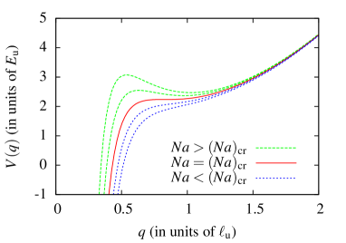
Figure 2: (Color online) Potential $V(q)$ in Eq. (16) for parameters $Na$ above, at, and below the critical value $(Na)_{\rm cr}$ of the tangent bifurcation.

We now show that the exceptional point at the critical value $Na=(Na)_{\rm cr}$ can be observed in the time evolution $q(t)$ of the condensate extension. In what follows we assume that the condensate is initially prepared in a stationary ground state at scattering length $Na\gtrsim(Na)_{\rm cr}$ and then the scattering length is decreased, in the computation or experimentally via tuning of a Feshbach resonance, in such a way that the mean-field energy of the excited state is below the energy of the initial state or the stationary states do not exist any more. In that case the condensate collapses, thereby crossing the inflection point of the potential $V(q)$ with vanishing second derivative.

To simplify the discussion we approximate $V(q)$ in the local vicinity of the inflection point by the parameter dependent cubic potential

$$U_{\alpha}(x)=x^{3}-\alpha x\;,$$ (17)

where the inflection point has been shifted to the origin. For $\alpha>0$ two stationary points exist at $x_{1,2}=\pm\sqrt{\alpha/3}$ and degenerate at the critical value $\alpha=\alpha_{\rm cr}=0$. The nonlinear equation of motion $\ddot{x}=-3x^{2}+\alpha$ for a particle (with mass $m=1$) moving in the potential (17) cannot be solved globally in terms of elementary functions. For initial conditions $x(0)=0$, $\dot{x}(0)=v_{0}$ and short times the solution can be expanded in a Taylor series

$$x(t)=v_{0}t+\frac{\alpha}{2}t^{2}+{\cal O}(t^{4})\;.$$ (18)

The Taylor expansion (18) does not show any special properties at the critical value $\alpha=0$. However, the properties of an exceptional point become evident when $x(t)$ is approximated by a sum of exponential functions,

$$x(t)\approx\sum_{k=1}^{n}d_{k}\exp(-\mathrm{i}\omega_{k}t)\;,$$ (19)

where the $d_{k}$ and $\omega_{k}$ are the amplitudes and frequencies of the signal, respectively (which both can be complex valued in general). Using the ansatz (19) is motivated by the fact that time signals for systems where the time propagation is described by linear operators are exactly given by a sum of exponential functions. The amplitudes and frequencies of a signal (19) can be extracted, even for large values of $n$, with the harmonic inversion method Wall and Neuhauser (1995); Mandelshtam and Taylor (1997a, b); Main (1999); Dž. Belkić et al. (2000); Fuchs et al. (2014). Here we choose $n=2$ which is sufficient to observe the degeneracy of two frequencies and obtain

$$d_{1,2} =\pm\frac{\mathrm{i}v_{0}^{2}}{\sqrt{3}\alpha}\quad,\quad\omega_{1,2}=\left(\mathrm{i}\pm\sqrt{3}\right)\frac{\alpha}{2v_{0}}\;.$$ (20)

The Taylor expansion of $x(t)$ in Eq. (19) with the parameters given in Eq. (20) agrees up to order $t^{3}$ with the Taylor series in Eq. (18). The existence of an exceptional point at the critical value $\alpha=0$ now becomes obvious from the amplitudes and frequencies of the signal (19) given in Eq. (20). For $\alpha=0$ the two frequencies coalesce at $\omega_{1}=\omega_{2}=0$ and both amplitudes $d_{1}$ and $d_{2}$ diverge. However, in the limit $\alpha\to 0$ the signal (19) converges to $x(t)\approx v_{0}t$ which can formally be written as

$$x(t)\approx(\tilde{d}_{0}+\tilde{d}_{1}t)\exp(-\mathrm{i}\omega t)\;,$$ (21)

with the single frequency $\omega=0$ and a prefactor in front of the exponential function which is a polynomial of degree one in $t$ with the coefficients $\tilde{d}_{0}=0$ and $\tilde{d}_{1}=v_{0}$. Exceptional points in time signals have been investigated in Fuchs et al. (2014), where it has been shown that the failure of the ansatz (19) due to diverging amplitudes and the occurrence of a term in the time signal given as the product of a polynomial of degree $n-1$ in time and an exponential function $\exp(-\mathrm{i}\omega_{k}t)$ is a clear signature of an exceptional point of order $n$. The frequencies and the coefficients of the polynomials can be extracted from the signal by the extended harmonic inversion method developed in Fuchs et al. (2014). The time evolution of $x(t)$ in Eq. (21) thus indicates the existence of a second order exceptional point.

The analysis of the motion of a particle in the cubic potential (17) can now be carried over to the analysis of the time-dependent extension of a condensate described by the potential (16) (see Fig. 2). A trajectory $q(t)$ crosses the potential region where the ground and excited state can coalesce at time $t_{0}$ determined by the condition $\dddot{q}(t_{0})=0$. When that point is shifted to the origin, i.e., $t\to t-t_{0}$ and $q(t)\to q(t)-q(t_{0})$ the analysis can be performed in the same way as described above for the cubic potential (17). The difference between the common applications of the harmonic inversion method to systems with linear time propagators and the analysis of the nonlinear dynamics of a particle, e.g., in the cubic potential (17) is that the time signal in the latter case is not globally given as a superposition of exponential functions, and therefore the analysis must be restricted to a local area in the time domain. For the numerical computation of the amplitudes and frequencies we resort to the harmonic inversion method as introduced in Fuchs et al. (2014).

As explained in Sec. II the description of the condensate dynamics with canonical coordinates and the Hamiltonian (14) is only possible for the simple but not very accurate variational approach to $\psi(\bm{r},t)$ using a single Gaussian function ($N_{g}=1$) in Eq. (2). Using the improved ansatz with coupled Gaussian functions the dynamics obtained from the equations of motion (3) for the variational parameters $A_{k}$ and $B_{k}$ cannot be described by an effective potential. However, we can still analyze the time evolution of the extension of the condensate wave function given as the root of the variance of the operator $\bm{r}$, i.e.

$$q(t)\equiv\sqrt{\langle\psi(t)|r^{2}|\psi(t)\rangle}\;,$$ (22)

which can be expressed in terms of the variational parameters [see Eq. (24) in the Appendix]. We use the notation $q(t)$ as in Eq. (15) although $q$ is not a canonical variable for coupled Gaussians. However, it is important to note that the extension of the condensate as defined in Eq. (22) is an observable and can be measured experimentally. The time evolution of $q(t)$ obtained with a single Gaussian function and with coupled Gaussians should qualitatively show a similar behavior, and thus can be analyzed in the same way using the harmonic inversion method to verify the existence of exceptional points. The results are presented and discussed in Sec. IV.

IV Results and discussion

To analyze the time evolution of the condensate a well defined initial wave function must be prepared which is not a stationary state of the Gross-Pitaevskii equation (1). A procedure which can be applied theoretically as well as experimentally is to prepare the stationary ground state of the condensate for a parameter $Na=s$ of the contact interaction and then suddenly to change the scattering length $a$. In an experiment the scattering length can be varied using Feshbach resonances. In what follows we present the results of numerical simulations with a condensate wave function described first by a single Gaussian function and then with coupled Gaussians.

IV.1 Approach with a single Gaussian function

In case of an ansatz with a single Gaussian function the ground state of the condensate for $Na=s$ can be determined as the local minimum of the potential $V(q)$ in Eq. (16). After changing the scattering length the equations of motion for the canonical coordinates $q$ and $p$ are obtained from the Hamiltonian (14) and can be integrated numerically. The trajectories $q(t)$ and the first derivatives $\dot{q}(t)$ for an initial state with $s=-0.665$ and various values of $Na$ in the range $-0.675\leq Na\leq-0.664$ are presented in Fig. 3. If the scattering length is not changed, i.e., $Na=s=-0.665$ then the extension of the condensate stays constant at $q(t)=0.8647$ in Fig. 3(a). A small change of the scattering length results in a breathing like dynamics of the wave function, a particle moving in the potential (16) (see Fig. 2) oscillates around the local minimum but the energy is not high enough to cross the barrier with the local maximum. That crossing is possible when $Na$ is reduced below $Na=-0.6693$. In this case $q(t)$ decreases monotonically and reaches $q=0$ [not shown in Fig. 3(a)] within finite time, which indicates the collapse of the condensate.

Are signatures of the exceptional point visible in Fig. 3? When the ground and excited state coalesce in the potential $V(q)$ in Fig. 2 the dynamics around the critical point is nearly a free motion linear in time, i.e., $q(t)=q(t_{0})+v_{0}(t-t_{0})+{\cal O}((t-t_{0})^{4})$. The nearly linear behavior can be seen when following the trajectory with $Na=-0.6705$ in Fig. 3(a) around $t=t_{0}=1.22$. The time derivative $\dot{q}(t)$ of that trajectory in Fig. 3(b) exhibits a saddle indicating the vanishing second and third derivative of $q(t)$ at $t=t_{0}$.

The clear identification of the exceptional point and the precise determination of the critical scattering length $(Na)_{\rm cr}$ is possible by analyzing the functions $q(t)$ as described in Sec. III. For each trajectory the time $t_{0}$ is computed where $\dddot{q}(t_{0})=0$. Some of these points are marked by plus symbols in Fig. 3(a). For the local harmonic inversion analysis we use only four signal points $c_{j}=q(t_{0}+j\Delta t)-q(t_{0})$ with $\Delta t=10^{-3}$ and $j=0,1,2,3$ to express this signal around $t=t_{0}$ as the sum of two exponential functions with two frequencies $\omega_{1,2}$ and amplitudes $d_{1,2}$. The results of the local harmonic inversion analysis are presented in Fig. 4. The states have been prepared with the initial parameter $Na=s=-0.57$ and then the time evolution of that state at a modified value $Na$ has been analyzed. As can be seen in Fig. 4(a) the real and imaginary parts of the frequencies intersect at the critical parameter $(Na)_{\rm cr}=-0.67051$, at that point the degenerate frequency is $\omega=0$. Note that the critical parameter agrees perfectly with the value given for $N_{g}=1$ in Table 1. The amplitudes $d_{1}$ and $d_{2}$ for the harmonic inversion analysis with an ansatz of two non-degenerate exponential functions are shown in Fig. 4(b). Both amplitudes diverge at $Na=(Na)_{\rm cr}$. By contrast, the coefficients $\tilde{d}_{0}$ and $\tilde{d}_{1}$ in a linear polynomial in $t$ for the ansatz (21) with a two-fold degenerate frequency do not show any singularities, as can be seen in Fig. 4(c), where the amplitudes $\tilde{d}_{0}$ and $\tilde{d}_{1}$ have been computed under the assumption of a single degenerate frequency $\omega\equiv(\omega_{1}+\omega_{2})/2$. As outlined in Fuchs et al. (2014) the nonzero linear coefficient $\tilde{d}_{1}=v_{0}$ at the critical parameter $Na=(Na)_{\rm cr}$, where the two frequencies are degenerate, is the signature of a second order exceptional point.

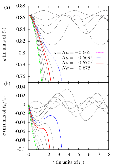
Figure 3: (Color online) (a) Trajectories $q(t)$ for the time evolution of the condensate extension computed with a single Gaussian function, $N_{g}=1$, and for various strengths $Na$ of the contact interaction in the range $-0.675\leq Na\leq-0.664$. A few trajectories are highlighted and labeled. The initial state of the condensate is prepared at $s=Na=-0.665$. The plus symbols indicate for some trajectories the points with vanishing third derivatives $\dddot{q}(t_{0})=0$. (b) Time derivatives $\dot{q}(t)$ of the trajectories in (a).

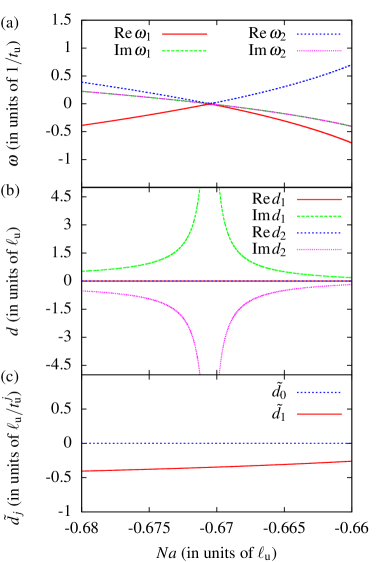
Figure 4: (Color online) (a) Frequencies and (b), (c) amplitudes obtained by the local harmonic inversion analysis of trajectories $q(t)$ computed with a single Gaussian function, $N_{g}=1$, and an initial state prepared at $s=Na=-0.57$. Note that $\mathrm{Im}\,\omega_{1}=\mathrm{Im}\,\omega_{2}$ and $\mathrm{Re}\,d_{1}=\mathrm{Re}\,d_{2}=0$ and thus the corresponding lines cannot be distinguished. See text for discussion.

IV.2 Approach with coupled Gaussians

The accuracy of the condensate wave function increases rapidly when using the ansatz in Eq. (2) with $N_{g}\geq 2$ coupled Gaussian functions. In that case the ground state of the BEC for $Na=s$ is computed as fixed point of the equations of motion (3) with a numerical root search as described in Rau et al. (2010b, c). After changing the scattering length the time dependence of the variational parameters $A_{k}$ and $B_{k}$ is obtained by numerical integration of the equations of motion (3). As shown in Fig. 1 and Table 1 the stationary states and the critical parameter $(Na)_{\textrm{cr}}$ converge rapidly with increasing number $N_{g}$ of Gaussian functions. Our calculations show a similar convergence behavior also for the time dependence of the trajectories $q(t)$, i.e., for given values $s$ and $Na$ trajectories computed with three or more Gaussian functions are nearly identical Brinker .

For an ansatz with $N_{g}=4$ coupled Gaussian functions and the parameter $s=Na=-0.57$ of the initial state the extension of the condensate as defined in Eq. (22) has been computed and the resulting trajectories $q(t)$ and first derivatives $\dot{q}(t)$ are presented in Fig. 5. The trajectories $q(t)$ computed with a single Gaussian function in Fig. 3(a) and with $N_{g}=4$ coupled Gaussians in Fig. 5(a) qualitatively appear to be very similar, however, subtle differences in the derivatives $\dot{q}(t)$ can be observed when comparing Figs. 3(b) and 5(b). The functions $\dot{q}(t)$ in Fig. 5(b) exhibit small fluctuations with higher frequencies which are absent in Fig. 3(b). The reason is that the dynamics of the condensate when computed with coupled Gaussian functions does not run exactly along the “reaction coordinate” corresponding to the coordinate $q$ in the one-dimensional potential (16) but oscillations in other degrees of freedom are slightly excited. Nonetheless, points with vanishing third derivatives $\dddot{q}(t_{0})=0$ can be determined and some of these points are marked by plus symbols in Fig. 5(a).

The results of the local harmonic inversion analysis of trajectories computed with $N_{g}=3$ coupled Gaussian functions are shown in Fig. 6. The degeneracy of the two frequencies at a critical value $Na=(Na)_{\rm cr}$ in Fig. 6(a) and the behavior of the amplitudes in Fig. 6(b) and (c) is similar as in Fig. 4, however, the exceptional point is shifted to the critical parameter value $(Na)_{\rm cr}=-0.57534$, which agrees very well with the value $(Na)_{\rm cr}=-0.57510$ for $N_{g}=3$ given in Table 1.

We have analyzed the collapse dynamics of condensates initially prepared at various strengths $s=Na$ of the contact interaction and computed the critical parameters $(Na)_{\rm cr}$ where the two frequencies $\omega_{1,2}$ coalesce and the amplitudes $d_{1,2}$ diverge. For $N_{g}=1$ the critical value of the exceptional point does not depend on the initial state, however, for coupled Gaussian functions the value of $(Na)_{\rm cr}$ slightly depends on $s$. This can be seen in Fig. 7 for $N_{g}=2$ and $N_{g}=3$.

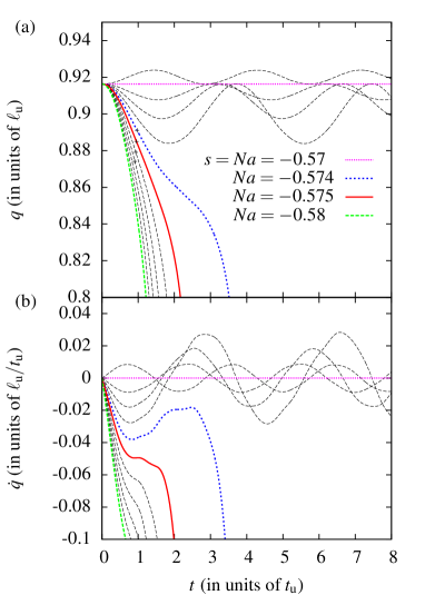
Figure 5: (Color online) (a) Trajectories $q(t)$ and (b) time derivatives $\dot{q}(t)$ as in Fig. 3 but computed with $N_{g}=4$ coupled Gaussian functions and the initial state prepared at $s=Na=-0.57$.

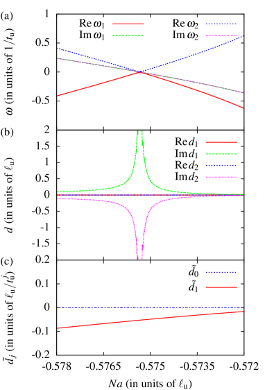
Figure 6: (Color online) (a) Frequencies and (b), (c) amplitudes obtained by the local harmonic inversion analysis of trajectories $q(t)$ as in Fig. 4 but computed with $N_{g}=3$ coupled Gaussian functions and the initial state prepared at $s=Na=-0.57$.

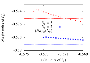
Figure 7: (Color online) Dependence of the critical parameter $(Na)_{\rm cr}$ on the strength $s=Na$ of the contact interaction of the initial state and the number of Gaussian functions $N_{g}$ used for the computations. The lines mark the values given in Table 1 for $N_{g}=2$ and $N_{g}=3$.

The dependence is caused by the excitation of fluctuations of the condensate in the various degrees of freedom as discussed above. However, the analysis of the collapse dynamics with $N_{g}=3$ coupled Gaussian functions allows one to determine the position of the exceptional point as $(Na)_{\rm cr}=-0.575\pm 0.001$, i.e., with an accuracy of about three significant digits.

The local harmonic inversion analysis of the collapse dynamics can be applied to verify experimentally the existence of an exceptional point in a BEC. In an experiment the initial state of the condensate can be prepared for a given parameter value $s=Na$ of the contact interaction, and then the scattering length is quickly ramped to a new value by using Feshbach resonances. The variance $\langle\psi(t)|r^{2}|\psi(t)\rangle$ of the condensate wave function after a delay time $t$ can be determined with the help of absorption images. Since the BEC is destroyed at the snapshot a sufficient number of identical condensates must be produced and absorption images must be taken at various delay times $t$ to obtain the time evolution $q(t)$ in Eq. (22).

V Conclusion

The time evolution of Bose-Einstein condensates described in the mean-field limit by the time-dependent nonlinear Gross-Pitaevskii equation differs completely from the behavior of quantum systems obeying the linear Schrödinger equation. Nevertheless, we have shown that signatures of exceptional points which are well known phenomena in non-Hermitian linear operators can be observed in the collapse dynamics of Bose-Einstein condensates. The verification of the exceptional points is possible using the local harmonic inversion analysis of the time evolution of the condensate extension during the collapse, and we propose the application of this method also for an experimental observation of exceptional points in BECs.

All computations in this Paper are based on the Gross-Pitaevskii equation obtained with a mean-field approximation. In calculations with a multi-orbital approach fragmented metastable states have been observed in the region $Na<(Na)_{\mathrm{cr}}$ Cederbaum et al. (2008); Tsatsos et al. (2010). An interesting question is whether the identification of exceptional points in this work can be related beyond the mean-field approach to the splitting of the ground state into multiple fragmented states.

In future studies it will also be interesting to detect critical phenomena in various time-dependent nonlinear systems by application of the local harmonic inversion analysis. The method may even be extended to observe bifurcation points or higher order exceptional points related to the coalescence of more than two stationary states in the dynamics of nonlinear systems.

Appendix A Gaussian integrals

For the ansatz with coupled Gaussian functions given in Eq. (2) the integrals required in Eq. (11) read

$$\braket{g_{k}}{g_{j}} =\frac{\mathrm{e}^{-(B_{j}+\bar{B}_{k})}\pi^{3/2}}{(A_{j}+\bar{A}_{k})^{3/2}}\,,$$ (23)

$$\braket{g_{k}}{r^{2}}{g_{j}} =\frac{3\mathrm{e}^{-(B_{j}+\bar{B}_{k})}\pi^{3/2}}{2(A_{j}+\bar{A}_{k})^{5/2}}\,,$$ (24)

$$\braket{g_{k}}{r^{4}}{g_{j}} =\frac{15\mathrm{e}^{-(B_{j}+\bar{B}_{k})}\pi^{3/2}}{4(A_{j}+\bar{A}_{k})^{7/2}}\,,$$ (25)

$$\braket{g_{k}}{}{\psi|^{2}|g_{j}} =\sum_{l,m=1}^{N_{g}}\frac{\mathrm{e}^{-(B_{j}+\bar{B}_{k}+B_{l}+\bar{B}_{m})}\pi^{3/2}}{(A_{j}+\bar{A}_{k}+A_{l}+\bar{A}_{m})^{3/2}}\,,$$ (26)

$$\braket{g_{k}}{r^{2}}{\psi|^{2}|g_{j}} =\sum_{l,m=1}^{N_{g}}\frac{3\mathrm{e}^{-(B_{j}+\bar{B}_{k}+B_{l}+\bar{B}_{m})}\pi^{3/2}}{2(A_{j}+\bar{A}_{k}+A_{l}+\bar{A}_{m})^{5/2}}\,.$$ (27)

The bars indicate the complex conjugate.

References

- Dalfovo and Stringari (1996) F. Dalfovo and S. Stringari, Phys. Rev. A 53, 2477 (1996).
- Pérez-García et al. (1997) V. M. Pérez-García, H. Michinel, J. I. Cirac, M. Lewenstein, and P. Zoller, Phys. Rev. A 56, 1424 (1997).
- Donley et al. (2001) E. A. Donley, N. R. Claussen, S. L. Cornish, J. L. Roberts, E. A. Cornell, and C. E. Wieman, Nature 412, 295 (2001).
- Huepe et al. (1999) C. Huepe, S. Métens, G. Dewel, P. Borckmans, and M. E. Brachet, Phys. Rev. Lett. 82, 1616 (1999).
- Huepe et al. (2003) C. Huepe, L. S. Tuckerman, S. Métens, and M. E. Brachet, Phys. Rev. A 68, 023609 (2003).
- Kato (1966) T. Kato, Perturbation theory for linear operators (Springer, Berlin, 1966).
- Moiseyev (2011) N. Moiseyev, Non-Hermitian Quantum Mechanics (Cambridge University Press, Cambridge, 2011).
- Latinne et al. (1995) O. Latinne, N. J. Kylstra, M. Dörr, J. Purvis, M. Terao-Dunseath, C. J. Joachain, P. G. Burke, and C. J. Noble, Phys. Rev. Lett. 74, 46 (1995).
- Korsch and Mossmann (2003) H. J. Korsch and S. Mossmann, J. Phys. A 36, 2139 (2003).
- Hernández et al. (2006) E. Hernández, A. Jáuregui, and A. Mondragón, J. Phys. A 39, 10087 (2006).
- Graefe et al. (2008) E. M. Graefe, U. Günther, H. J. Korsch, and A. E. Niederle, J. Phys. A 41, 255206 (2008).
- von Brentano and Philipp (1999) P. von Brentano and M. Philipp, Phys. Lett. B 454, 171 (1999).
- Oberthaler et al. (1996) M. K. Oberthaler, R. Abfalterer, S. Bernet, J. Schmiedmayer, and A. Zeilinger, Phys. Rev. Lett. 77, 4980 (1996).
- Shuvalov and Scott (2000) A. L. Shuvalov and N. H. Scott, Acta Mech. 140, 1 (2000).
- Berry (1994) M. V. Berry, Curr. Sci. 67, 220 (1994).
- Klaiman et al. (2008) S. Klaiman, U. Günther, and N. Moiseyev, Phys. Rev. Lett. 101, 080402 (2008).
- Wiersig et al. (2008) J. Wiersig, S. W. Kim, and M. Hentschel, Phys. Rev. A 78, 053809 (2008).
- Philipp et al. (2000) M. Philipp, P. von Brentano, G. Pascovici, and A. Richter, Phys. Rev. E 62, 1922 (2000).
- Dembowski et al. (2003) C. Dembowski, B. Dietz, H.-D. Gräf, H. L. Harney, A. Heine, W. D. Heiss, and A. Richter, Phys. Rev. Lett. 90, 034101 (2003).
- Dietz et al. (2007) B. Dietz, T. Friedrich, J. Metz, M. Miski-Oglu, A. Richter, F. Schäfer, and C. A. Stafford, Phys. Rev. E 75, 027201 (2007).
- Poston and Stewart (1978) T. Poston and I. Stewart, Catastrophe Theory and its Applications (Pitman Publishing Limited, London, 1978).
- Cartarius et al. (2008a) H. Cartarius, J. Main, and G. Wunner, Phys. Rev. A 77, 013618 (2008a).
- Rapedius and Korsch (2009) K. Rapedius and H. J. Korsch, J. Phys. B 42, 044005 (2009).
- O’Dell et al. (2000) D. O’Dell, S. Giovanazzi, G. Kurizki, and V. M. Akulin, Phys. Rev. Lett. 84, 5687 (2000).
- Cartarius et al. (2008b) H. Cartarius, T. Fabčič, J. Main, and G. Wunner, Phys. Rev. A 78, 013615 (2008b).
- Griesmaier et al. (2005) A. Griesmaier, J. Werner, S. Hensler, J. Stuhler, and T. Pfau, Phys. Rev. Lett. 94, 160401 (2005).
- Koch et al. (2008) T. Koch, T. Lahaye, J. Metz, B. Fröhlich, A. Griesmaier, and T. Pfau, Nature Physics 4, 218 (2008).
- Lahaye et al. (2008) T. Lahaye, J. Metz, B. Fröhlich, T. Koch, M. Meister, A. Griesmaier, T. Pfau, H. Saito, Y. Kawaguchi, and M. Ueda, Phys. Rev. Lett. 101, 080401 (2008).
- Lahaye et al. (2009) T. Lahaye, C. Menotti, L. Santos, M. Lewenstein, and T. Pfau, Rep. Prog. Phys. 72, 126401 (2009).
- Köberle et al. (2009) P. Köberle, H. Cartarius, T. Fabčič, J. Main, and G. Wunner, New J. Phys. 11, 023017 (2009).
- Gutöhrlein et al. (2013) R. Gutöhrlein, J. Main, H. Cartarius, and G. Wunner, J. Phys. A: Math. Theor. 46, 305001 (2013).
- Skryabin (2000) D. V. Skryabin, Phys. Rev. A 63, 013602 (2000).
- Kawaguchi and Ohmi (2004) Y. Kawaguchi and T. Ohmi, Phys. Rev. A 70, 043610 (2004).
- Kreibich et al. (2012) M. Kreibich, J. Main, and G. Wunner, Phys. Rev. A 86, 013608 (2012).
- Kreibich et al. (2013) M. Kreibich, J. Main, and G. Wunner, J. Phys. B 46, 045302 (2013).
- Haag et al. (2014) D. Haag, D. Dast, A. Löhle, H. Cartarius, J. Main, and G. Wunner, Phys. Rev. A 89, 023601 (2014).
- Löhle et al. (2014) A. Löhle, H. Cartarius, D. Haag, D. Dast, J. Main, and G. Wunner, Acta Polytech. 54, 133 (2014).
- Stehmann et al. (2004) T. Stehmann, W. D. Heiss, and F. G. Scholtz, J. Phys. A: Math. Gen. 37, 7813 (2004).
- Cartarius and Moiseyev (2011) H. Cartarius and N. Moiseyev, Phys. Rev. A 84, 013419 (2011).
- Uzdin et al. (2013) R. Uzdin, E. G. Dalla Torre, R. Kosloff, and N. Moiseyev, Phys. Rev. A 88, 022505 (2013).
- Fuchs et al. (2014) J. Fuchs, J. Main, H. Cartarius, and G. Wunner, J. Phys. A: Math. Theor. 47, 125304 (2014).
- Pitaevskii and Stringari (2003) L. P. Pitaevskii and S. Stringari, Bose-Einstein Condensation (Oxford University Press, Oxford, 2003).
- Rau et al. (2010a) S. Rau, J. Main, P. Köberle, and G. Wunner, Phys. Rev. A 81, 031605(R) (2010a).
- Rau et al. (2010b) S. Rau, J. Main, and G. Wunner, Phys. Rev. A 82, 023610 (2010b).
- Rau et al. (2010c) S. Rau, J. Main, H. Cartarius, P. Köberle, and G. Wunner, Phys. Rev. A 82, 023611 (2010c).
- Eichler et al. (2011) R. Eichler, J. Main, and G. Wunner, Phys. Rev. A 83, 053604 (2011).
- Marquardt et al. (2012) K. Marquardt, P. Wieland, R. Häfner, H. Cartarius, J. Main, and G. Wunner, Phys. Rev. A 86, 063629 (2012).
- McLachlan (1964) A. D. McLachlan, Mol. Phys. 8, 39 (1964).
- Wall and Neuhauser (1995) M. R. Wall and D. Neuhauser, J. Chem. Phys. 102, 8011 (1995).
- Mandelshtam and Taylor (1997a) V. A. Mandelshtam and H. S. Taylor, Phys. Rev. Lett. 78, 3274 (1997a).
- Mandelshtam and Taylor (1997b) V. A. Mandelshtam and H. S. Taylor, J. Chem. Phys. 107, 6756 (1997b).
- Main (1999) J. Main, Phys. Rep. 316, 233 (1999).
- Dž. Belkić et al. (2000) Dž. Belkić, P. A. Dando, J. Main, and H. S. Taylor, J. Chem. Phys. 113, 6542 (2000).
- (54) J. Brinker, Bachelor thesis, Universität Stuttgart, 2014 (unpublished). URL: http://itp1.uni-stuttgart.de/publikationen/abschlussarbeiten/brinker_bachelor_2014.pdf.
- Cederbaum et al. (2008) L. S. Cederbaum, A. I. Streltsov, and O. E. Alon, Phys. Rev. Lett. 100, 040402 (2008).
- Tsatsos et al. (2010) M. C. Tsatsos, A. I. Streltsov, O. E. Alon, and L. S. Cederbaum, Phys. Rev. A 82, 033613 (2010).