Rescaling Ward identities in the random normal matrix model

Abstract.

We study existence and universality of scaling limits for the eigenvalues of a random normal matrix, in particular at points on the boundary of the spectrum. Our approach uses Ward’s equation – an integro-differential identity satisfied by the rescaled one-point function.

In random normal matrix theory, one studies normal matrices $M$ (i.e. $MM^{*}=M^{*}M$) of some large order $n$ picked randomly with respect to a probability measure of the form

(0.1) $$d\mu_{n}(M)=\frac{1}{\mathcal{Z}_{n}}\,e^{\,-n\operatorname{tr}Q(M)}\,dM.$$

Here $dM$ is the surface measure on normal $n\times n$ matrices inherited from $4n^{2}$-dimensional Lebesgue measure via the natural embedding into ${\mathbb{C}}^{\,n^{2}}$, $Q(\zeta)$ is a suitable real-valued function defined on ${\mathbb{C}}$ ("large” as $\zeta\to\infty$), and $\mathcal{Z}_{n}$ is a normalizing constant; $\operatorname{tr}Q(M)=\sum_{1}^{n}Q(\zeta_{j})$ is the usual trace of the matrix $Q(M)$, where $\zeta_{j}$ denote the eigenvalues.

If $Q$ is just defined on ${\mathbb{R}}$ and $dM$ is surface measure on the Hermitian matrices (i.e. $M^{*}=M$), one obtains random Hermitian matrices. The study of such eigenvalue ensembles, e.g. using the technique of Riemann-Hilbert problems, has been an active area of research.

The eigenvalues $\{\zeta_{j}\}_{1}^{n}$ of a normal matrix $M$, picked randomly with respect to the measure (0.1), form a random point process in the complex plane ${\mathbb{C}}$. The same point processes also appear as a special case of one-component plasma (or "OCP”) ensembles, where $\{\zeta_{j}\}_{1}^{n}$ has the interpretation of a system of repelling point charges subjected to the external field $nQ$. Here the factor $n$ is needed to ensure that the system stays in a finite portion of the plane as $n\to\infty$.

In either interpretation, one defines the "energy” of the system $\{\zeta_{j}\}_{1}^{n}$ by

(0.2) $$H_{n}\left(\zeta_{1},\ldots,\zeta_{n}\right)=\sum_{j\neq k}\log\frac{1}{\left|{\,\zeta_{j}-\zeta_{k}\,}\right|}+n\sum_{j=1}^{n}Q\left(\zeta_{j}\right).$$

The joint distribution of the particles/eigenvalues then follows the the Boltzmann-Gibbs law,

(0.3) $$d{\mathbb{P}}_{n}(\zeta)=\frac{1}{Z_{n}}\,e^{\,-\,H_{n}(\zeta)}\,dV_{n}(\zeta),\quad\zeta=(\zeta_{1},\ldots,\zeta_{n})\in{\mathbb{C}}^{n},$$

where $dV_{n}$ is Lebesgue measure in ${\mathbb{C}}^{n}$ divided by $\pi^{n}$, and $Z_{n}=\int e^{\,-\,H_{n}}\,dV_{n}$. We can henceforth treat the system $\{\zeta_{j}\}_{1}^{n}$ simply as a random sample from the distribution (0.3), having the interpretations as random eigenvalues or as point charges. An important feature of this process is that it is determinantal.

As $n\to\infty$, the system $\{\zeta_{j}\}_{1}^{n}$ tends to occupy a certain set $S$ called the droplet. More precisely, the empirical distribution $\frac{1}{n}\sum_{1}^{n}\delta_{\zeta_{j}}$ converges in a suitable sense [28] to the equilibrium measure given by weighted potential theory. In addition, the fluctuations of the system about the equilibrium converges to the Gaussian field on $S$ with free boundary conditions. See [2].

In this paper we will study microscopic properties of the system, close to a point $p$ in the droplet; in particular, a boundary point. The figure below shows a random sample from the classical Ginibre ensemble, in which $Q=\left|{\,\zeta\,}\right|^{\,2}$ and $S=\left\{\,\zeta\,;\,\left|{\,\zeta\,}\right|\leq 1\,\right\}$. In this case, the process $\{\zeta_{j}\}_{1}^{n}$ can alternatively be interpreted as the eigenvalues of an $n\times n$ matrix whose entries are independent complex, centered Gaussian random variables of variance $1/n$, see [26].

We rescale about the point $p=1$ by letting $z_{j}=\sqrt{n}\,\left(\zeta_{j}-1\right)$ and refer to the rescaled system $\Theta_{n}=\{z_{j}\}_{1}^{n}$ as the free boundary Ginibre process.

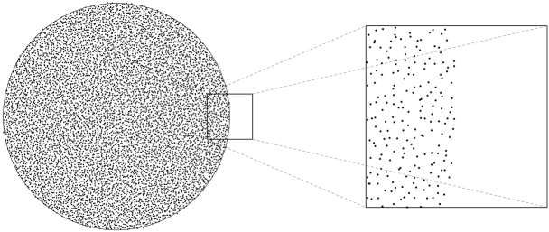
Figure 1. A sample of the free boundary Ginibre process for a large value of $n$

The processes $\Theta_{n}$ converge as $n\to\infty$ to a determinantal random point field in ${\mathbb{C}}$ with correlation kernel

(0.4) $$K(z,w)=G(z,w)F\left(z+\bar{w}\right),$$

where we call $G(z,w):=e^{\,z\bar{w}\,-|\,z\,|^{\,2}/2\,-|\,w\,|^{\,2}/2}$ the Ginibre kernel and $F(z):=\frac{1}{2}\operatorname{erfc}\left(\frac{z}{\sqrt{2}}\right)$ the free boundary plasma function. To the best of our knowledge, this formula for the limiting point field first appeared in the paper [24] by Forrester and Honner; a rigorous proof was given in the paper [13]. (An alternative, simple argument depending on normal approximation of the Poisson distribution is given in Section 2.)

We shall prove that the kernel (0.4) appears "universally” at regular points of the boundary, at least under an additional assumption of "translation invariance”. This condition is satisfied e.g. when $Q$ is radially symmetric. In a certain sense, (0.4) is an analogue to the Airy kernel in Hermitian random matrix theory, i.e.,

(0.5) $$K(x,y)=\frac{\operatorname{Ai}(x)\operatorname{Ai}^{\prime}(y)-\operatorname{Ai}^{\prime}(x)\operatorname{Ai}(y)}{x-y},$$

which describes the eigenvalue spacing at the edge of the spectrum. See [7, 9, 22, 44] and the references there for further information.

We will also establish existence and some basic properties of sequential limiting point fields pertaining to a quite general $Q$ at an arbitrary point of the droplet. It is here useful to allow the point to vary with $n$, i.e., we can equally well zoom in on a "moving point”. This device is used in a separate paper [5] to study the distribution of eigenvalues near singular boundary points.

Our approach uses a relation between the $1$- and $2$-point functions, a particular case of Ward identities for Boltzmann-Gibbs ensembles. This relation is well-known in field theories [32] and has also been used in the papers [2, 31] to study fluctuations of eigenvalues.

We here fix some point on the boundary and rescale Ward’s identity about that point. It turns out that, if this is done properly, then limiting one- and two-point functions $R=R_{1}$ and $R_{2}$ can be defined in a way so that the Berezin kernel

$$B(z,w):=\frac{R(z)R(w)-R_{2}(z,w)}{R(z)}$$

satisfies the equation

(0.6) $${\bar{\partial}}C=R-1-{\partial}{\bar{\partial}}\log R,\quad\text{where}\quad C(z):=\frac{1}{\pi}\int_{\mathbb{C}}\frac{B(z,w)}{z-w}\,d^{2}\,w.$$

We refer to the equation (0.6) as Ward’s equation. We stress that this equation is valid at all (moving) points, provided that $\Delta Q$ does not vanish there and that $R$ does not vanish identically.

It is more or less immediate from the computations with the Ginibre ensemble that the correlation kernel (0.4) gives rise to a solution to Ward’s equation. However, in order to have uniqueness of solution to Ward’s equation, we need to impose certain conditions, which depend on the nature of the point we are rescaling about. Our verification of these conditions uses the formula for the expectation of linear statistics from [2], and some Bergman space techniques.

The method of rescaled Ward identities applies to some other situations as well. We shall for example consider hard edge ensembles, where we completely confine the system $\{\zeta_{j}\}_{1}^{n}$ to the droplet by setting $Q=+\infty$ outside of $S$. In this case, a new kernel arises at regular boundary points: the hard edge plasma kernel

(0.7) $$K(z,w)=G(z,w)H(z+\bar{w})\,{\chi}_{\mathbb{L}}(z)\,{\chi}_{\mathbb{L}}(w),\quad H(z)=\frac{1}{\sqrt{2\pi}}\int_{-\infty}^{\,0}\frac{e^{\,-\,\left(z-t\right)^{\,2}/2}}{F(t)}\,dt,$$

where ${\chi}_{\mathbb{L}}$ is the indicator function for the left half plane ${\mathbb{L}}=\{\,z\,;\,\operatorname{Re}z<0\,\}$, and $F$ is the free boundary plasma function.

Figure 2. The graphs of $F$ and $H$, restricted to the reals.

We will here give an elementary derivation of the formula for the case of the hard edge Ginibre ensemble. For reasons of length, it is convenient to postpone a complete treatment, including universality, to the companion paper [4]. We remark that the hard edge kernel plays a role somewhat similar to the Bessel kernel in Hermitian random matrix theory

$$K(x,y)=\frac{J_{0}(\sqrt{x}\,)\sqrt{y}\,J_{0}^{\prime}(\sqrt{y}\,)-\sqrt{x}\,J_{0}^{\prime}(\sqrt{x}\,)J_{0}(\sqrt{y}\,)}{2(x-y)}.$$

See e.g. [24, 44, 56] and the references there.

A detailed description of our results is given in the following section.

Notational conventions

By $D(\zeta;r)$ we denote the open disc with center $\zeta$ and radius $r$. We write ${\partial}\omega$, $\operatorname{Int}\omega$, $\operatorname{cl}\omega$, and $\omega^{c}$ for the boundary, the interior, and the complement of a set $\omega\subset{\mathbb{C}}$. The indicator function of a set $E$ is denoted by ${\chi}_{E}$. We write ${\partial}=\frac{1}{2}\left({\partial}/{\partial}x-i{\partial}/{\partial}y\right)$ and ${\bar{\partial}}=\frac{1}{2}\left({\partial}/{\partial}x+i{\partial}/{\partial}y\right)$ for the complex derivatives and $\Delta={\partial}{\bar{\partial}}$ for the normalized Laplacian. Thus $\Delta$ is $\frac{1}{4}$ times the standard Laplacian. We write $dA(z)=d^{\,2}z/\pi$ for normalized Lebesgue measure. Thus the unit disc has measure $1$. The volume measure on ${\mathbb{C}}^{k}$ is defined by $dV_{k}(\zeta_{1},\ldots,\zeta_{k})=dA(\zeta_{1})\cdots dA(\zeta_{k})$.

A continuous function $f:{\mathbb{C}}^{2}\to{\mathbb{C}}$ is termed Hermitian if $f(z,w)=\overline{f(w,z)}$. We shall say that $f$ is Hermitian-analytic (or Hermitian-entire) if $f$ is Hermitian and analytic (resp. entire) as a function of $z$ and $\bar{w}$. A Hermitian-entire function is uniquely determined by its diagonal values $f(z,z)$.

A Hermitian function $c$ is called a cocycle if

$$c(z_{1},z_{2})c(z_{2},z_{3})\cdots c(z_{k-1},z_{k})c(z_{k},z_{1})=1$$

for all $k\geq 1$ and all sequences $(z_{j})_{1}^{k}$. Alternatively, $c$ is a cocycle iff $c(z,w)=g(z)\overline{g(w)}$ for a continuous unimodular function $g$.

1. Introduction and results

1.1. Potential theory and droplets

Fix a suitable function ("external potential”) $Q:{\mathbb{C}}\to{\mathbb{R}}\cup\{+\infty\}$. Let ${\mathcal{P}}$ denote the class of positive, compactly supported Borel measures on ${\mathbb{C}}$.

Define the weighted logarithmic energy of $\mu\in{\mathcal{P}}$ in external field $Q$ by

$$I_{Q}\left[\mu\right]=\iint_{{\mathbb{C}}^{2}}\log\frac{1}{\left|{\,\zeta-\eta\,}\right|}\,d\mu(\zeta)\,d\mu(\eta)+\int_{\mathbb{C}}Q\,d\mu.$$

Thinking of $\mu$ as the distribution of an electric charge, $I_{Q}[\mu]$ is the sum of the Coulomb interaction energy and the energy of interaction of $\mu$ with the external field $Q$.

We always assume that $Q$ is lower semi-continuous, and that $Q$ is finite on some set of positive logarithmic capacity. We will also assume that $Q$ is sufficiently large at infinity, in the sense that

$$Q(\zeta)>>\log\left|{\,\zeta\,}\right|,\qquad(\zeta\to\infty).$$

To be precise, it will suffice to assume that $\liminf_{\zeta\to\infty}Q\left(\zeta\right)/\log\left|{\,\zeta\,}\right|>2$.

A classical theorem of Frostman states that there then exists a unique equilibrium measure $\sigma$ which minimizes the weighted energy,

$$I_{Q}[\sigma]=\min_{\mu({\mathbb{C}})=1}I_{Q}[\mu],\qquad(\mu\in{\mathcal{P}}).$$

See [47]. We denote the compact support of the equilibrium measure by

$$S=S\left[Q\right]=\operatorname{supp}\sigma.$$

We refer to $S$ as the droplet in the external field $Q$. It is known that if $Q$ is smooth in some neighbourhood of $S$, then $\sigma$ is absolutely continuous and takes the explicit form (see [47])

(1.1) $$d\sigma={\chi}_{S}\cdot\Delta Q\,dA.$$

Since $\sigma$ is a probability measure, we have $\Delta Q\geq 0$ on $S$.

Our main assumptions throughout are that there is some neighbourhood $\Omega$ of $S$ such that

1. $Q$ is real analytic in $\Omega$,

2. $\Delta Q>0$ in $\Omega$.

With these assumptions, the complement $S^{c}$ has a local Schwarz function at each boundary point, and we can rely on the fundamental theorem of Sakai [48] concerning domains with local Schwarz functions. In particular, we can apply Sakai’s regularity theorem, which implies that all but finitely many boundary points $p\in{\partial}S$ are regular in the sense that there is a disc $D=D(p;\epsilon)$ such that $D\setminus S$ is a Jordan domain and $D\cap({\partial}S)$ is a simple real analytic arc. A non-regular point $p\in{\partial}S$ is called a singular boundary point. Such points can be classified further as cusps or double points. We shall here study the regular case and refer to [5] for the singular case.

1.2. Rescaling eigenvalue ensembles

Fix a potential $Q$ as above, and let $(\zeta_{j})_{1}^{n}$ denote a point in ${\mathbb{C}}^{n}$ picked randomly with respect to the measure ${\mathbb{P}}_{n}$ in (0.3). We refer to the corresponding (unordered) configuration $\{\zeta_{j}\}_{1}^{n}$ as the $n$-point process (or simply "system”) associated to $Q$. We also speak of $\{\zeta_{j}\}_{1}^{n}$ as a "configuration picked randomly with respect to ${\mathbb{P}}_{n}$”.

To each Borel set $B$ in ${\mathbb{C}}$ we associate a random variable $N_{B}$ by $N_{B}=\#\left\{\,j\,;\,\zeta_{j}\in B\,\right\}$. The system $\{\zeta_{j}\}_{1}^{n}$ is then determined by the set of joint intensities (a.k.a. "correlation functions”)

(1.2) $${\mathbf{R}}_{n,k}\left(\eta_{1},\ldots,\eta_{k}\right)=\lim_{\varepsilon\downarrow 0}\frac{{\mathbb{P}}_{n}\left(\,\bigcap_{j=1}^{k}\left\{\,N_{D(\eta_{j};\varepsilon)}\geq 1\,\right\}\,\right)}{\varepsilon^{2k}},\qquad k=1,\ldots,n,\quad n\in{\mathbb{Z}}_{+}.$$

A few comments are in order.

The Hamiltonian $H(\zeta_{1},\ldots,\zeta_{n})$ is defined as $+\infty$ when $\zeta_{j}=\zeta_{k}$ for distinct $j$ and $k$. It is then easy to see that the limit in (1.2) exists, at least when the points $\eta_{1},\ldots,\eta_{k}$ are away from eventual discontinuities of $Q$. Moreover, ${\mathbf{R}}_{n,k}(\eta_{1},\ldots,\eta_{k})=0$ when $\eta_{i}=\eta_{j}$ for some distinct indices $i,j\leq k$.

The joint intensities are non-negative symmetric functions, subject to the relations

(1.3) $$\int_{\mathbb{C}}{\mathbf{R}}_{n,1}\,dA=n;\qquad\int_{\mathbb{C}}{\mathbf{R}}_{n,k+1}\left(\eta_{1},\ldots,\eta_{k},\eta_{k+1}\right)\,dA\left(\eta_{k+1}\right)=\left(n-k\right)\,{\mathbf{R}}_{n,k}\left(\eta_{1},\ldots,\eta_{k}\right).$$

We sometimes identify the intensity ${\mathbf{R}}_{n,k}$ with the measure ${\mathbf{R}}_{n,k}\,dV_{k}$.

According to Dyson’s determinant formula the joint intensities can be represented in the form

$${\mathbf{R}}_{n,k}(\zeta_{1},\ldots,\zeta_{k})=\det\left({\mathbf{K}}_{n}(\zeta_{i},\zeta_{j})\right)_{i,j=1}^{k}$$

where ${\mathbf{K}}_{n}$ is a Hermitian function known as a correlation kernel of the process. A proof of this formula, written for the case of Hermitian random matrices, is given e.g. in [47], Section IV.7.2. A proof in the case of normal matrices runs in the same way.

We are interested in microscopic properties of the system $\{\zeta_{j}\}_{1}^{n}$ near a point $p\in S$. It is natural to magnify distances about $p$ by a factor $\sqrt{n\Delta Q(p)}$ and fix an angle $\theta\in{\mathbb{R}}$. We shall consider rescaled point processes of the form $\Theta_{n}=\Theta_{n}(p,\theta)=\{z_{j}\}_{1}^{n}$, where

(1.4) $$z_{j}=e^{\,-i\theta}\sqrt{n\Delta Q(p)}\,\left(\zeta_{j}-p\right),\quad j=1,\ldots,n.$$

The law of $\Theta_{n}$ is defined as the image of the Boltzmann-Gibbs measure (0.3) under the map (1.4). The rescaled system $\Theta_{n}$ then has intensities denoted $R_{n,k}$, where

$$R_{n,k}\left(z_{1},\ldots,z_{k}\right)=\frac{1}{\left(n\Delta Q(p)\right)^{k}}\,{\mathbf{R}}_{n,k}\left(\zeta_{1},\ldots,\zeta_{k}\right).$$

We shall henceforth usually assume that $p$ is a regular boundary point. We then throughout, by convention, take $e^{i\theta}$ as the outer normal to ${\partial}S$ at $p$.

The point process $\Theta_{n}$ is determinantal with kernel $K_{n}$ given by

$$K_{n}(z,w)=\frac{1}{n\Delta Q(p)}{\mathbf{K}}_{n}(\zeta,\eta),\quad\text{where}\quad\begin{cases}\,z=e^{\,-i\theta}\sqrt{n\Delta Q(p)}\,\left(\zeta-p\right)\cr w=e^{\,-i\theta}\sqrt{n\Delta Q(p)}\,\left(\eta-p\right)\cr\end{cases},$$

The fundamental problem is existence and uniqueness of a limiting determinantal point field of the processes $\Theta_{n}$, as $n\to\infty$. For our purposes, convergence will mean locally uniform convergence of all intensities $R_{n,k}$ to some limits $R_{k}$ as $n\to\infty$. Whenever this is the case, $R_{k}$ can be interpreted in terms of Lenard’s theory (see [53]) as a $k$-point function for a "point field” in ${\mathbb{C}}$, meaning a probability law on a suitable space of (perhaps) infinite configurations $\{z_{i}\}_{1}^{\infty}\subset{\mathbb{C}}$. A precise definition, and a discussion of relevant convergence results, is given in the appendix.

It here suffices to note that the desired convergence of the processes $\Theta_{n}$ will hold if the correlation kernels $K_{n}$ converge to a limit $K$ locally uniformly on ${\mathbb{C}}^{2}$. Moreover, the limiting point field is uniquely determined by $K$ if the functions $K_{n}(z,z)$ are uniformly bounded, and it is then determinantal with intensity functions

$$R_{k}(z_{1},\ldots,z_{k})=\det\left(K(z_{i},z_{j})\right)_{i,j=1}^{k}.$$

More generally, if $K_{n}$ is a correlation kernel and $(c_{n})_{1}^{\infty}$ is a sequence of cocycles, then $c_{n}K_{n}$ is another kernel giving rise to the same joint intensities $R_{n,k}$. The problem is thus to show that there exists a sequence of cocycles such that $c_{n}K_{n}$ converges locally uniformly to a non-trivial limit $K$ with bounded convergence on the diagonal in ${\mathbb{C}}^{2}$.

The best understood case is when $p\in\operatorname{Int}S$. Then, under the much weaker assumption that $Q$ is $C^{2}$-smooth near $p$, the rescaled processes $\Theta_{n}$ converge to the Ginibre$(\infty)$ point field. The correlation kernel of this field is the Ginibre kernel,

(1.5) $$G(z,w)=e^{\,z\bar{w}\,-\,\left|{\,z\,}\right|^{\,2}/2\,-\,\left|{\,w\,}\right|^{\,2}/2}.$$

If $p\in\operatorname{Int}S$, and if we rescale about $p$ according to (1.4) with arbitrary angle $\theta$, then we have

$$R_{n,k}\left(z_{1},\ldots,z_{k}\right)\to\det\left(G\left(z_{i},z_{j}\right)\right)_{i,j=1}^{k}\qquad\text{as}\quad n\to\infty$$

with locally uniform convergence on ${\mathbb{C}}^{k}$. (Cf. [1]; a new proof is given in Section 7.6.)

In the following sections, we will state the main results of the paper.

1.3. Compactness, non-triviality, and Ward’s equation

Our first theorem states the existence of sequential limits of the rescaled point processes $\Theta_{n}$ and specifies the form of limiting correlation kernels. With a view to later applications [5] we shall adopt a somewhat broader point of view, rescaling about a moving point $p=(p_{n})_{1}^{\infty}$ where $p_{n}$ is a sequence of points in $S$. A constant sequence $p_{n}=p$ will be identified with the point $p$. In the following result we are also at liberty to choose a sequence of angles $\theta_{n}\in{\mathbb{R}}$ and rescale about $p$ according to

(1.6) $$z_{j}=e^{-i\theta_{n}}\sqrt{n\Delta Q(p_{n})}\left(\zeta_{j}-p_{n}\right).$$

Theorem A.

Let $p\in S$ be a (possibly moving) point, and rescale about $p$ as above.

1. Compactness: There is a sequence $c_{n}$ of cocycles such that every subsequence of $\left(c_{n}K_{n}\right)_{1}^{\infty}$ has a subsequence converging uniformly on compact subsets.

2. Analyticity: Each limit point in (i) satisfies $K=G\Psi$ where $\Psi$ is a Hermitian entire function which satisfies the following "mass-one inequality”:

   (1.7) $$\int_{\mathbb{C}}e^{\,-\,|\,z-w\,|^{\,2}}\left|{\,\Psi(z,w)\,}\right|^{\,2}\,dA(w)\leq\Psi(z,z).$$

A limit point $K$ in Theorem A will be called a limiting kernel. It follows from (i) that $K$ is a positive matrix in Aronszajn’s sense [8], i.e., for all finite sequences $(z_{j})_{1}^{N}$ of points and all choices of scalars $(\alpha_{j})_{1}^{N}$ we have

$$\sum_{j,k=1}^{N}\alpha_{j}\bar{\alpha}_{k}K(z_{j},z_{k})\geq 0.$$

Indeed, $K$ is a limit of $c_{n_{k}}K_{n_{k}}$ where $K_{n}$ are positive matrices and $c_{n}$ are cocycles. Moreover, by the general theory mentioned in the previous section, a limiting kernel $K$ is the correlation kernel of a some point field in the plane, which we call a limiting point field. The $1$-point function of this point field is denoted by $R(z)=K(z,z)$. If $R\neq 0$ on ${\mathbb{C}}$ we can define the Berezin kernel

$$B(z,w)=\frac{\left|\,K(z,w)\,\right|^{\,2}}{K(z,z)},$$

and the "Cauchy transform”

(1.8) $$C(z)=\int_{\mathbb{C}}\frac{B(z,w)}{z-w}\,dA(w).$$

Theorem B.

Let $K=G\Psi$ be a limiting kernel in Theorem A and write $R(z)=K(z,z)$. Let $p\in S$ be a (possibly moving) point.

1. Zero-one law: Either $R$ is trivial, in the sense that $R=0$ identically, or $R>0$ everywhere.

2. Ward’s equation: If $R$ is non-trivial, then the integral $C(z)$ in (1.8) converges and defines a smooth function such that

   $${\bar{\partial}}C(z)=R(z)-1-\Delta\log R(z),\qquad z\in{\mathbb{C}}.$$

3. Complementarity: The "complementary kernel”

   $$\tilde{K}(z,w):=G(z,w)(1-\Psi(z,w))$$

   is a positive matrix. In particular, $R(z)=\Psi(z,z)\leq 1$ for all $z$.

In connection with the zero-one law, we mention that triviality (i.e. $R=0$) occurs when one rescales about singular boundary points. See [5].

As a word of warning, we mention that the complementary kernel does not in general solve Ward’s equation.

By the preceding results, it is natural to try to find all (or at least some) limiting kernels $K$ giving rise to a solution to Ward’s equation. In order to fix a solution uniquely, we need to know that certain additional conditions are satisfied, which depend on the nature of the point we are rescaling about. For regular points, the results are as follows.

Theorem C.

Fix a regular boundary point $p$ and let $K$ be a corresponding limiting kernel in Theorem A. Write $x=\operatorname{Re}z$.

1. Exterior estimate: There is a constant $C$ such that

   $$R(z)\leq C\,e^{\,-\,2\,x^{\,2}}\quad\text{for}\quad x\geq 0.$$

2. Interior estimate: If $\ell$ is any number with $\ell<1/2$ then there is a constant $C$ (perhaps depending on $\ell$) such that

   $$\left|{\,R(z)-1\,}\right|\leq C\,e^{\,-\,\ell\,x^{\,2}}\quad\text{for}\quad x\leq 0.$$

We believe that the interior estimate (ii) should be true with $\ell=2$. However, the exact value of $\ell$ is not important in the sequel.

Theorem D.

Suppose that the droplet $S$ is connected with everywhere regular boundary ${\partial}S$. Then there is a subset $N\subset{\partial}S$ of measure zero for the arclength such that if $K$ is a limiting rescaled kernel about a point $p\in({\partial}S)\setminus N$, then $R(x)=K(x,x)$ satisfies

$$\int_{-\infty}^{+\infty}x\cdot(R(x)-{\chi}_{(-\infty,0)}(x))\,dx=\frac{1}{8}.$$

In particular, the foregoing results imply that any limiting kernel at a regular boundary point is non-trivial, i.e. $R(z)>0$ for all $z$. Moreover, as $R$ is bounded, we can conclude that all limiting point fields are uniquely determined by the corresponding limiting kernel.

The topological assumptions on the droplet in Theorem D are made in order to be able to use the fluctuation theorem from [2]; the theorem should be true without this assumption.

1.4. Translation invariant solutions to Ward’s equation

Let $K=G\Psi$ be a limiting kernel in Theorem A. We say that $\Psi$ (or $K=G\Psi$) is (vertical) translation invariant (in short: t.i. ) if

$$\Psi\left(z+it,w+it\right)=\Psi\left(z,w\right),\qquad t\in{\mathbb{R}}.$$

In this case, $\Psi$ can be represented in the form

$$\Psi(z,w)=\Phi(z+\bar{w})$$

for some entire function $\Phi$. To study kernels of this form, it is convenient to introduce the "Gaussian kernel”

$$\gamma(z):=\frac{1}{\sqrt{2\pi}}\,e^{\,-\,z^{\,2}/2},\qquad z\in{\mathbb{C}}.$$

Let $g$ be a bounded function on ${\mathbb{R}}$. We shall use the symbol "$*$” to denote the convolution operation

$$\gamma*g(z):=\int_{-\infty}^{+\infty}\gamma\left(z-t\right)g(t)\,dt,\qquad z\in{\mathbb{C}}.$$

Thus $\gamma*g$ has the meaning of ordinary convolution in ${\mathbb{R}}$ followed by analytic continuation. The function $z\mapsto(\gamma*g)(z)\cdot e^{z^{2}/4}$ is a version of the Bargmann transform of $g$ (see e.g. [22]). Note that the free boundary plasma function $F$ can be written

(1.9) $$F(z)=\gamma*{\chi}_{(-\infty,0)}(z)=\int_{-\infty}^{\,0}\gamma\left(z-t\right)\,dt.$$

The convolution operation is intimately connected with t.i. limiting kernels. Indeed, if $K(z,w)=G(z,w)\Phi(z+\bar{w})$ is an arbitrary t.i. limiting kernel, then we shall prove that there exists a Borel function $f$ with $0\leq f\leq 1$ such that $\Phi=\gamma*f$. Our proof of this fact relies on Bochner’s theorem on positive definite functions; see Section 6.1.

We will refer to the formula $\Phi=\gamma*f$ as the Gaussian representation of the t.i. limiting kernel $K$. Our next theorem says that $f$ is necessarily a characteristic function.

Theorem E.

Suppose that $\Phi$ is an entire function of the form $\Phi=\gamma*f$ where $f$ is a bounded function. Then the kernel $K(z,w)=G(z,w)\Phi(z+\bar{w})$ gives rise to a solution to Ward’s equation if and only if there is a connected set $I\subset{\mathbb{R}}$ of positive measure such that $\Phi=\gamma*{\chi}_{I}$.

By Theorem C, a t.i. limiting kernel $K(z,w)=G(z,w)\Phi(z+\bar{w})$ must be of the form $\Phi=\gamma*{\chi}_{(-\infty,a)}$ for some $a\in{\mathbb{R}}$. It is easy to show that the only choice of $a$ consistent with the $1/8$-formula in Theorem D is $a=0$. See Section 6.3 for details. Thus we will have $\Phi=F$ at almost every boundary point, provided e.g. that the droplet $S$ is connected and having everywhere regular boundary.

In general, we do not know whether all limiting kernels necessarily are t.i. It is however easy to show that this is the case when the potential is radially symmetric, i.e., when $Q(z)=Q(|z|)$.

Theorem F.

Suppose that $Q$ is radially symmetric and that the droplet $S$ is connected. For a boundary point $p$ we let $\Theta_{n}$ be the free boundary process rescaled about $p$ in the outer normal direction. Then $\Theta_{n}$ converges to the unique point field $BG$ in ${\mathbb{C}}$ with the correlation kernel

(1.10) $$K(z,w)=G(z,w)\cdot F\left(z+\bar{w}\right).$$

The topological assumption means that the droplet is either a disc or an annulus. This restriction should be regarded as a technical assumption made in order to apply Theorem D.

We will call the kernel $K$ in (1.10), resp. the point field $BG$, the "boundary Ginibre” kernel/point field. It is a natural conjecture that $BG$ is universal at regular boundary points for all potentials. After this note was completed, the convergence was verified for the non-symmetric potentials ("ellipse ensembles”) $Q=|\,\zeta\,|^{\,2}-t\operatorname{Re}(\zeta^{\,2})$, $0<t<1$. See [36]. The verification depends on explicit computations with the orthogonal polynomials, which were obtained in the thesis [46].

1.5. Berezin kernel and mass-one equation

Let $B_{n}$ be the Berezin kernels of the rescaled processes $\Theta_{n}$, i.e.,

$$B_{n}(z,w)=\frac{R_{n,1}(z)R_{n,1}(w)-R_{n,2}(z,w)}{R_{n,1}(z)}=\frac{\left|{\,K_{n}(z,w)\,}\right|^{\,2}}{K_{n}(z,z)}.$$

We have (e.g. by (1.3))

(1.11) $$\int_{\mathbb{C}}B_{n}(z,w)\,dA(w)=1.$$

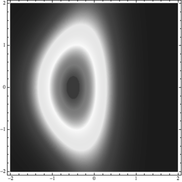
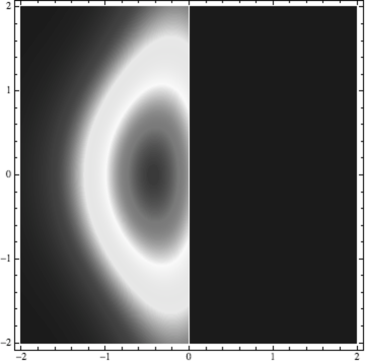
Figure 3. The Berezin kernel $B_{n}(0,w)$ for the free boundary Ginibre ensemble, and its hard edge counterpart, for a large value of $n$.

Let us write $R_{n}=R_{n,1}$ and denote by $R_{n-1}^{\,(a)}$ the $1$-point function for the conditional $(n-1)$-point process $\Theta_{n}|\left\{a\in\Theta_{n}\right\}$. For each fixed $a\in{\mathbb{C}}$, we then have

(1.12) $$B_{n}(a,w)=R_{n}(w)-R_{n-1}^{\,(a)}(w).$$

(For details, see [1], Section 7.6.)

It is natural to ask whether the relation (1.11) also holds for the limiting kernel $B=\lim_{n}B_{n}$.

Figure 4 shows the Berezin kernel corresponding to the boundary Ginibre ensembles. In this case, direct computations show that $\int B(a,w)\,dA(w)=1$ and so we have

$$R^{\,(a)}(z)=R(z)-B(a,z)=F(2x)-e^{\,-\,\left|{\,z-a\,}\right|^{\,2}}\left|{\,F(a+z)\,}\right|^{\,2}/F(2a),\qquad z=x+iy,$$

The corresponding conditional $1$-point function rescaled about a bulk point is $z\mapsto 1-e^{\,-\,\left|{\,z-a\,}\right|^{\,2}}$.

Elementary calculations now show that if we rescale about the point $p$ and insert a point charge at $a=0$, then the repulsion caused if $p$ is in the bulk is stronger, by a factor $\pi/(\pi-2)\approx 3$, compared to if the point $p$ is on the boundary.

Let us say that a limiting kernel $K=G\Psi$ satisfies the mass-one equation if the corresponding Berezin kernel $B$ satisfies $\int_{\mathbb{C}}B(z,w)\,dA(w)=1$ for all $z$, i.e.,

$$\int_{\mathbb{C}}e^{\,-\,\left|{\,z-w\,}\right|^{\,2}}\left|{\,\Psi(z,w)\,}\right|^{\,2}\,dA(w)=\Psi(z,z),\qquad z\in{\mathbb{C}}.$$

This equation is technically similar to Ward’s equation and it has a simple spectral interpretation (see Section 7.4). Every kernel $K$ giving rise to a solution to the mass-one equation is furthermore a correlation kernel of some point field.

In view of the Gaussian representability of t.i. limiting kernels, it is natural to study solutions to the mass-one equation of the form $\Phi=\gamma*f$ where $f$ is a bounded function on ${\mathbb{R}}$. Of course, such solutions do not necessarily correspond to actual limiting kernels.

The following theorem describes all solutions of this form.

Theorem G.

Let $\Phi=\gamma*f$ where $f$ is a bounded Borel function on ${\mathbb{R}}$, and put $\Psi(z,w)=\Phi(z+\bar{w})$. Then $\Psi$ gives rise to a solution to the mass-one equation if and only if there is a Borel set $e\subset{\mathbb{R}}$ of positive measure such that $f={\chi}_{e}$.

A noteworthy consequence of our theory is that all non-trivial t.i. limiting kernels satisfy the mass-one equation. This follows by combining theorems B, E, and G.

1.6. Organization of the paper

In Section 2 we consider the boundary Ginibre ensembles, both for the free boundary and the hard edge. We give a short proof of the convergence of rescaled ensembles to the boundary Ginibre point fields with kernels (0.4) and (0.7), respectively.

In Section 3, we prove Theorem A (compactness and analyticity).

In Section 4 we derive Ward’s equation and prove Theorem B.

In Section 5, we establish a priori bounds for regular points (Theorem C). We also prove the $1/8$-formula in Theorem D at almost every boundary point.

In Section 6 we specialize to t.i. solutions and prove theorems E, F, and G.

The last section, Section 7, contains various concluding remarks. In particular, we comment on the nature of the mass-one and Ward equations, we show that these equations take the form of twisted convolution equations, we discuss Hilbert spaces of entire functions associated to limiting kernels, and write down versions of Ward’s equation in some settings which are different from the free boundary case studied in this paper (hard edge, bulk singularities, $\beta$-ensembles).

2. Example: The Ginibre ensembles

2.1. Principles of notation

Consider first a general potential $Q$. By a weighted polynomial of order $n$ we mean a function of the form $f=q\cdot e^{-nQ/2}$ where $q$ is an (analytic) polynomial of degree at most $n-1$. Let $\mathcal{W}_{n}$ denote the space of all weighted polynomials of order $n$, considered as a subspace of $L^{2}=L^{2}({\mathbb{C}},dA)$. It is well-known that the reproducing kernel ${\mathbf{K}}_{n}(\zeta,\eta)$ for the space $\mathcal{W}_{n}$ is a correlation kernel for the process $\{\zeta_{j}\}_{1}^{n}$ corresponding to $Q$. This implies that one has the formula

(2.1) $$\mathbf{K}_{n}(\zeta,\eta)=\sum_{j=0}^{n-1}q_{j}(\zeta)\,\bar{q}_{j}(\eta)\,e^{\,-nQ(\zeta)/2-nQ(\eta)/2},$$

where $q_{j}$ is the $j$:th orthonormal polynomial with respect to the measure $e^{-nQ(\zeta)}dA(\zeta)$.

Recall the Ginibre potential $Q=\left|\,\zeta\,\right|^{\,2}$. The corresponding droplet is $S=\left\{\,\zeta\,;\,\left|\,\zeta\,\right|\leq 1\,\right\}$.

We shall give an elementary proof for $BG$-convergence using Poisson approximation of the normal distribution. Our proof is quite similar to the argument in the paper [45], where the spectral radius of a Ginibre matrix is studied. Let us mention also that there are several other proofs of BG convergence for the free boundary Ginibre ensemble.

2.2. Free boundary Ginibre ensemble

Let $\{\zeta_{j}\}_{1}^{n}$ denote a random configuration for the free boundary Ginibre process. We rescale about the boundary point $p=1$ in the outer normal direction, via $z_{j}=\sqrt{n}\left(\zeta_{j}-1\right)$, writing $\Theta_{n}=\{z_{j}\}_{1}^{n}$ for the rescaled process. Let $G$ and $F$ be the Ginibre kernel and the free boundary plasma function, respectively. See (1.5) and (1.9). We shall prove the following theorem, found in [24] (cf. [13]).

Theorem 2.1.

There exists a unique point field $BG$ with correlation kernel $K(z,w)=G(z,w)F(z+\bar{w})$, and the processes $\Theta_{n}$ converge to $BG$ as $n\to\infty$ with locally uniform convergence of intensity functions.

Since $K(z,z)<1$, it suffices to prove the statement about convergence of intensity functions.

By (2.1), a correlation kernel for the process $\{\zeta_{j}\}_{1}^{n}$ is computed to

(2.2) $${\mathbf{K}}_{n}(\zeta,\eta)=n\sum_{j=0}^{n-1}\frac{\left(n\zeta\bar{\eta}\right)^{j}}{j!}e^{\,-n\frac{\left|{\,\zeta\,}\right|^{\,2}+\left|{\,\eta\,}\right|^{\,2}}{2}}.$$

Now rescale according to

$$\zeta=1+z/\sqrt{n}\quad,\quad\eta=1+w/\sqrt{n}.$$

and note that the rescaled process $\Theta_{n}$ has correlation kernel $K_{n}(z,w)=\frac{1}{n}{\mathbf{K}}_{n}\left(\zeta,\eta\right).$ Using (2.2), we write $K_{n}$ in the form

$$K_{n}(z,w)=\sum_{j=0}^{n-1}\left(\frac{n\zeta\bar{\eta}}{\lambda}\right)^{j}\frac{\lambda^{j}}{j!}e^{\,-\lambda}$$

where

(2.3) $$\lambda=\lambda(n)=\frac{n}{2}\left(|\,\zeta\,|^{\,2}+|\,\eta\,|^{\,2}\right)=n+\sqrt{n}\operatorname{Re}(z+w)+\frac{1}{2}\left(|\,z\,|^{\,2}+|\,w\,|^{\,2}\right).$$

We next let $X_{n}$ be a Poisson distributed random variable with intensity $\lambda=\lambda(n)$ (in short: $X_{n}\sim\text{Po}(\lambda)$), i.e.,

$${\mathbb{P}}\left\{X_{n}=k\right\}=\frac{\lambda^{k}}{k!}e^{\,-\,\lambda},\quad k=0,1,\ldots.$$

We then have the identity

$$K_{n}(z,w)={\mathbb{E}}\left[\left(\frac{n\zeta\bar{\eta}}{\lambda}\right)^{X_{n}}\cdot{\chi}_{\left\{X_{n}<n\right\}}\right].$$

Now introduce a new random variable $Y_{n}$ by

$$X_{n}=\lambda+\sqrt{\lambda}\,Y_{n}.$$

By the central limit theorem, $Y_{n}$ converges in distribution to the standard normal as $n\to\infty$; the convergence is moreover uniform. (This is the well-known "normal approximation of the Poisson distribution”; uniform convergence follows e.g. by the Berry-Esseen theorem.)

Now factorize $K_{n}(z,w)$ in the following way,

(2.4) $$K_{n}(z,w)=A_{n}\cdot B_{n}:=\left(\frac{n\zeta\bar{\eta}}{\lambda}\right)^{\lambda}\cdot{\mathbb{E}}\left[\left(\frac{n\zeta\bar{\eta}}{\lambda}\right)^{\sqrt{\lambda}\cdot Y_{n}}\cdot{\chi}_{\left\{Y_{n}<\alpha_{n}\right\}}\right],$$

where

$$\alpha_{n}=\frac{n-\lambda}{\sqrt{\lambda}}.$$

Note that $\alpha_{n}\to-\operatorname{Re}(z+w)$ as $n\to\infty$.

Lemma 2.2.

We have the convergence

$$B_{n}\to e^{\,-b^{2}/2}F(z,w)\quad\text{as}\quad n\to\infty,$$

where $b=b(z,w)=\operatorname{Im}(z+\bar{w})$ and $F$ is the free boundary kernel (1.9). Moreover,

$$A_{n}=e^{\,ib\sqrt{n}}e^{\,b^{2}/2}G(z,w)(1+o(1))$$

where $G$ is the Ginibre kernel and $o(1)\to 0$ uniformly on compact sets as $n\to\infty$.

Proof.

By a straightforward calculation we have

(2.5) $$\frac{n\zeta\bar{\eta}}{\lambda}=1+\frac{i}{\sqrt{n}}\operatorname{Im}(z+\bar{w})+\frac{1}{n}a+O\left(n^{-3/2}\right)$$

where

$$a=a(z,w)=z\bar{w}-(z+\bar{w})\operatorname{Re}(z+w)-\frac{1}{2}\left(|\,z\,|^{\,2}+|\,w\,|^{\,2}\right)+\left[\operatorname{Re}(z+w)\right]^{\,2}.$$

Inserting these expressions into $B_{n}$ (see (2.4)) using the fact that the $Y_{n}$ are asymptotically normal, we now approximate as follows (the symbol "$\sim$” stands for asymptotic equality as $n\to\infty$)

$$B_{n} \sim\frac{1}{\sqrt{2\pi}}\int_{-\infty}^{\,\alpha_{n}}\left(1+\frac{i}{\sqrt{n}}\operatorname{Im}(z+\bar{w})+O(1/n)\right)^{\sqrt{n}\cdot t}\,e^{\,-\,t^{\,2}/2}\,dt$$

$$\sim\frac{1}{\sqrt{2\pi}}\int_{-\infty}^{\,-\operatorname{Re}(z+\bar{w})}e^{\,i\operatorname{Im}(z+\bar{w})t}e^{\,-\,t^{\,2}/2}\,dt=e^{\,-\,b^{\,2}/2}\cdot F(z+\bar{w}).$$

We now turn to the factor $A_{n}$ in (2.4). To deal with it, we denote $c=\operatorname{Re}(z+w)$. By (2.5), we then have

$$A_{n}=\left(1+\frac{ib}{\sqrt{n}}+\frac{a}{n}+O\left(n^{-3/2}\right)\right)^{n+c\sqrt{n}+O(1)}=e^{\,ib\sqrt{n}}\,e^{\,b^{\,2}/2}\,e^{\,ibc+a}\,e^{\,o(1)}.$$

Noting that

$$ibc+a=z\bar{w}-\frac{1}{2}\left(|\,z\,|^{\,2}+|\,w\,|^{\,2}\right),$$

we finish the proof of the lemma. ∎

By the lemma and relation (2.4), we have

$$K_{n}(z,w)=e^{\,i\sqrt{n}\operatorname{Im}(z-w)}K(z,w)(1+o(1))$$

where $K$ is the free boundary kernel defined in (1.10). Since the factor $c_{n}(z,w)=e^{i\sqrt{n}\operatorname{Im}(z-w)}$ is a cocycle, this factor can be dropped when computing intensity functions $R_{n,k}(z)=\det(K_{n}(z_{i},z_{j}))$. This proves the desired convergence of intensity functions, at the same time establishing existence and uniqueness of the field $BG$. The proof of Theorem 2.1 is complete. ∎

2.3. Hard edge Ginibre ensemble

Let $Q^{S}(z)=\left|{\,z\,}\right|^{\,2}$ when $|\,z\,|\leq 1$ and $Q^{S}=+\infty$ otherwise. Let $\{\zeta_{i}\}_{1}^{n}$ denote a random configuration from the corresponding ensemble. Rescaling about $p=1$ via $z_{j}=\sqrt{n}\,(\zeta_{j}-1)$ we obtain a process $\Theta_{n}$. Let $H$ be the hard edge plasma function (0.7).

Theorem 2.3.

There exists a unique point field $BG_{h}$ with correlation kernel

$$K(z,w)=G(z,w)H(z+\bar{w})\,({\chi}_{\mathbb{L}}\otimes{\chi}_{\mathbb{L}})(z,w).$$

The processes $\Theta_{n}$ converge to $BG_{h}$ in the sense that all intensity functions converge locally boundedly almost everywhere, and locally uniformly in ${\mathbb{L}}^{2}$, to the intensity functions of $BG_{h}$.

Note that $K(z,z)<2$ for all $z$. We prove in the appendix that the convergence of intensity functions in the theorem implies the existence and uniqueness of a field $BG_{h}$ with correlation kernel $K$. It thus suffices to prove convergence.

By (2.1) and a calculation, a correlation kernel for the hard edge Ginibre process is given by

$$\mathbf{K}_{n}(\zeta,\eta)=n\sum_{j=0}^{n-1}\frac{(n\zeta\bar{\eta})^{j}}{\gamma\left(j+1,n\right)}e^{\,-nQ^{S}\left(\zeta\right)/2-nQ^{S}\left(\eta\right)/2},$$

where $\gamma\left(j+1,n\right)=\int_{0}^{n}s^{j}e^{-s}\,ds$ is the lower incomplete Gamma function. Now rescale by

$$\zeta=1+z/\sqrt{n}\quad,\quad\eta=1+w/\sqrt{n},\qquad z,w\in{\mathbb{L}}$$

and write

$$K_{n}(z,w)=\frac{1}{n}\mathbf{K}_{n}(\zeta,\eta)=\sum_{j=0}^{n-1}\left(\frac{n\zeta\bar{\eta}}{\lambda}\right)^{j}\frac{\lambda^{j}}{\gamma\left(j+1,n\right)}e^{-\lambda},$$

where $\lambda=n(|\,\zeta\,|^{\,2}+|\,\eta\,|^{\,2})/2$ is as in (2.3). We shall use a rough estimate for $\gamma(j+1,n)$. Observe that, by a well-known fact, we have

$$\gamma\left(j+1,n\right)=j!\left(1-e^{-n}\sum_{k=0}^{j}\frac{n^{k}}{k!}\right)=j!{\mathbb{P}}\left(U_{n}>j\right)$$

where $U_{n}\sim\text{Po}(n)$. By normal approximation of the Poisson distribution

$${\mathbb{P}}\left(U_{n}>j\right)={\varphi}\left(\xi_{j,n}\right)(1+o(1)),$$

where ${\varphi}(\xi)=\frac{1}{\sqrt{2\pi}}\int_{\xi}^{\infty}e^{-t^{2}/2}\,dt$, $\xi_{j,n}=(j-n)/\sqrt{n}$, and and $o(1)\to 0$ as $n\to\infty$ uniformly in $j$. We have shown that

$$K_{n}(z,w)=(1+o(1))\sum_{j=0}^{n-1}\left(\frac{n\zeta\bar{\eta}}{\lambda}\right)^{j}\frac{\lambda^{j}}{j!}e^{-\lambda}\frac{1}{{\varphi}(\xi_{j,n})}.$$

Finally, if $X_{n}\sim\text{Po}(\lambda)$, we can write the last sum in the form

$$\sum_{j=0}^{n-1}\left(\frac{n\zeta\bar{\eta}}{\lambda}\right)^{j}\frac{1}{{\varphi}(\xi_{j,n})}{\mathbb{P}}(X_{n}=j)={\mathbb{E}}\left[\left(\frac{n\zeta\bar{\eta}}{\lambda}\right)^{X_{n}}\cdot\frac{1}{{\varphi}\left(\frac{X_{n}-n}{\sqrt{n}}\right)}\cdot{\chi}_{\left\{X_{n}<n\right\}}\right].$$

Defining $Y_{n}$ by $X_{n}=\lambda+\sqrt{\lambda}Y_{n}$, we now get a relation of the form

$$K_{n}(z,w) =(1+o(1))\left(\frac{n\zeta\bar{\eta}}{\lambda}\right)^{\lambda}\cdot{\mathbb{E}}\left[\left(\frac{n\zeta\bar{\eta}}{\lambda}\right)^{\sqrt{\lambda}Y_{n}}\frac{1}{{\varphi}\left(\sqrt{\lambda/n}Y_{n}\,-\alpha_{n}\right)}\cdot{\chi}_{\left\{Y_{n}<\alpha_{n}\right\}}\right]$$

$$=(1+o(1))A_{n}\cdot\tilde{B}_{n},\qquad\alpha_{n}=(n-\lambda)/\sqrt{\lambda}.$$

Using the asymptotic identities $\alpha_{n}\sim-\operatorname{Re}(z+w)$ and $\lambda/n\sim 1$, we approximate the factor $\tilde{B}_{n}$ as follows, using the central limit theorem,

$$\tilde{B}_{n} \sim\frac{1}{\sqrt{2\pi}}\int_{-\infty}^{\,-\operatorname{Re}(z+w)}e^{\,i\operatorname{Im}(z+\bar{w})t}\frac{1}{{\varphi}\left(\sqrt{\lambda/n}\,t-\alpha_{n}\right)}e^{\,-\,t^{\,2}/2}\,dt$$

$$\sim e^{\,-\,b^{\,2}/2}\frac{1}{\sqrt{2\pi}}\int_{-\infty}^{\,-\,\operatorname{Re}(z+w)}\frac{1}{{\varphi}\left(\,\operatorname{Re}(z+\bar{w})+t\,\right)}e^{\,-\,\left(t-i\operatorname{Im}(z+\bar{w})\right)^{\,2}/2}\,dt$$

$$=e^{\,-\,b^{\,2}/2}\frac{1}{\sqrt{2\pi}}\int_{-\infty}^{\,0}\frac{1}{{\varphi}(u)}e^{\,-\,\left(u-(z+\bar{w})\right)^{\,2}/2}\,du=e^{\,-\,b^{\,2}/2}H(z+\bar{w}).$$

Using the asymptotics for $A_{n}$ in Lemma 2.2 we now conclude that

$$K_{n}(z,w)=e^{\,i\sqrt{n}\operatorname{Im}(z-w)}G(z,w)H(z+\bar{w})(1+o(1)),\quad z,w\in{\mathbb{L}},$$

where $o(1)\to 0$ uniformly on compacts. The first factor is a cocycle. We conclude that if $K(z,w)=G(z,w)H(z+\bar{w}){\chi}_{\mathbb{L}}(z){\chi}_{\mathbb{L}}(w)$ is the hard edge kernel, then $K_{n}\to K$ almost everywhere with locally bounded convergence, finishing the proof of the theorem. q.e.d.

3. Analyticity and compactness

In this section, we prove Theorem A. We thus fix a moving point $p=(p_{n})\in S$ and a sequence of angles $\theta_{n}$ and rescale about $p$ according to

$$z_{n}=e^{-i\theta_{n}}\sqrt{n\Delta Q(p_{n})}(\zeta-p_{n}).$$

To simplify notation we shall in the following write $p$ for $p_{n}$ and $\theta$ for $\theta_{n}$. The careful reader will note that all our estimates are independent of $n$.

3.1. General notation

For a measurable function $\phi:{\mathbb{C}}\to{\mathbb{R}}\cup\{+\infty\}$ we define $L^{2}_{\phi}$ to be the space of functions normed by

$$\left\|\,f\,\right\|_{\phi}^{\,2}=\int_{\mathbb{C}}\left|\,f\,\right|^{\,2}e^{\,-\,\phi}\,dA.$$

When $\phi=0$ we just write $L^{2}$ for $L^{2}_{\phi}$ and denote the norm by $\|\cdot\|$.

We denote by $C$ (large) and $c$ (small) various positive unspecified constants (independent of $n$) whose exact value can change meaning from time to time.

3.2. Potentials and reproducing kernels

Fix a neighbourhood $\Omega$ of $S$ and a number $\delta_{0}>0$ such that $Q$ is real-analytic and strictly subharmonic in the $2\delta_{0}$-neighbourhood of $\Omega$.

Let ${\mathcal{P}}_{n}$ be the space of analytic polynomials of degree at most $n-1$; we equip ${\mathcal{P}}_{n}$ with the norm of $L^{2}_{nQ}$. The corresponding space $\mathcal{W}_{n}$ of weighted polynomials is defined to consist of all functions of the form $f=qe^{\,-\,nQ/2}$ where $q\in{\mathcal{P}}_{n}$; we regard $\mathcal{W}_{n}$ as a subspace of $L^{2}$ and denote the corresponding orthogonal projections by

$$\pi_{n}:L^{2}_{nQ}\to{\mathcal{P}}_{n}\qquad\text{and}\qquad\Pi_{n}:L^{2}\to\mathcal{W}_{n}.$$

We write $\mathbf{k}_{n}$ and ${\mathbf{K}}_{n}$ for the reproducing kernels of ${\mathcal{P}}_{n}$ and $\mathcal{W}_{n}$ respectively. Then

$${\mathbf{K}}_{n}(\zeta,\eta)=\mathbf{k}_{n}(\zeta,\eta)e^{\,-\,nQ(\zeta)/2}e^{\,-\,nQ(\eta)/2}.$$

It is easy to see that the assignment

$$U_{n}:L^{2}_{nQ}\to L^{2}\qquad:\qquad f\mapsto fe^{\,-\,nQ/2}$$

is unitary, maps ${\mathcal{P}}_{n}$ onto $\mathcal{W}_{n}$, and satisfies $U_{n}\pi_{n}=\Pi_{n}U_{n}$.

3.3. Analytic continuation and bulk approximations

Let $A(\zeta,\eta)$ be a Hermitian-analytic function defined in a neighbourhood in ${\mathbb{C}}^{2}$ of the "diagonal” $X:=\left\{\,(\zeta,\zeta)\,;\,\zeta\in\Omega\,\right\}$, such that

$$A(\zeta,\zeta)=Q(\zeta),\quad\zeta\in\Omega.$$

We can choose $\delta_{0}>0$ small enough that $A(\zeta,\eta)$ is defined and Hermitian-analytic in the set of points $(\zeta,\eta)\in{\mathbb{C}}^{2}$ whose distance to $X$ is $<2\delta_{0}$. Call this set $\Lambda$.

We now define "bulk approximations” $\mathbf{k}_{n}^{\#}$ and ${\mathbf{K}}_{n}^{\#}$, defined in the domain of $A(\zeta,\eta)$ via

(3.1) $$\mathbf{k}_{n}^{\#}(\zeta,\eta)=n\left({\partial}_{1}\bar{{\partial}}_{2}A\right)(\zeta,\eta)\cdot e^{\,nA(\zeta,\eta)}\qquad\text{and}\qquad{\mathbf{K}}_{n}^{\#}(\zeta,\eta)=\mathbf{k}_{n}^{\#}(\zeta,\eta)e^{\,-\,nQ(\zeta)/2}e^{\,-\,nQ(\eta)/2}.$$

3.4. Elementary estimates for the one-point function

We write ${\mathbf{R}}_{n}(\zeta)={\mathbf{K}}_{n}(\zeta,\zeta)$ for the one-point function. By a basic fact for reproducing kernels we have the identity

(3.2) $${\mathbf{R}}_{n}(\zeta)=\sup\left\{\,\left|\,f(\zeta)\,\right|^{\,2}\,;\,f\in\mathcal{W}_{n}\,,\,\left\|\,f\,\right\|\leq 1\,\right\}.$$

We shall also use the following simple pointwise-$L^{2}$ estimate.

Lemma 3.1.

Suppose that $u$ is analytic in the disc $D:=D\left(p;c/\sqrt{n\Delta Q(p)}\right)$, where $Q$ is $C^{2}$-smooth at $p$. Let $f=ue^{-\,nQ/2}$. Then there is a number $C$ depending only on $c$ and $\Delta Q(p)$ such that

$$\left|{\,f(p)\,}\right|^{\,2}\leq Cn\int_{D}\left|{\,f\,}\right|^{\,2}\,dA.$$

Proof.

Suppose w.l.o.g. that $\Delta Q(p)=1$ and pick a number $a>1$. Consider the function $F_{n}(z)=f\left(p+z/\sqrt{n}\right)\cdot e^{a\left|{\,z\,}\right|^{\,2}/2}$. We then have $\Delta\log\left|{\,F(z)\,}\right|^{\,2}\geq-\Delta Q\left(p+z/\sqrt{n}\right)+a\geq 0$ for $\left|{\,z\,}\right|\leq c$ if $n$ is large enough. Then $F_{n}$ is subharmonic in $D$, which implies the desired estimate. ∎

Let $\gamma$ be the minimum of $Q+2U^{\sigma}$, where $U^{\sigma}(z)=\int_{\mathbb{C}}\log\frac{1}{\left|{\,z-w\,}\right|}\,d\sigma(w)$ is the logarithmic potential of the equilibrium measure $\sigma=\Delta Q\cdot{\chi}_{S}\,dA$. By the obstacle function corresponding to $Q$, we mean the subharmonic function

$$\check{Q}\left(\zeta\right)=-2U^{\sigma}\left(\zeta\right)+\gamma.$$

It is known (see [47]) that $\check{Q}=Q$ on $S$ while $\check{Q}$ is harmonic on $S^{c}$ and is of logarithmic increase

$$\check{Q}\left(\zeta\right)=\log\left|{\,\zeta\,}\right|^{\,2}+O(1),\qquad(\zeta\to\infty).$$

Furthermore $\check{Q}$ has a Lipschitz continuous gradient on ${\mathbb{C}}$. We remind of the following basic result; the "maximum principle of weighted potential theory”.

Lemma 3.2.

If $f\in{\mathcal{W}}_{n}$ and $\left|{\,f\,}\right|\leq 1$ on $S$, then $\left|{\,f\,}\right|\leq e^{\,-\,n\left(Q-\check{Q}\right)/2}$ on ${\mathbb{C}}$.

Proof.

If $f=p\cdot e^{-nQ/2}$, then $\frac{1}{n}\log\left|{\,p\,}\right|^{\,2}$ is a subharmonic minorant of $Q$ which grows no faster than $\log\left|{\,\zeta\,}\right|^{\,2}+{\textrm{const.}}$ as $\zeta\to\infty$. It is well-known that $\check{Q}(\zeta)$ is the supremum of $f(\zeta)$ where $f$ ranges over the functions having these properties (see e.g. [47]). ∎

Combining the preceding lemmas with the identity (3.2) gives the following bound for the $1$-point function.

Lemma 3.3.

There is a constant $C$ independent of $n$ and $\zeta$ such that

$${\mathbf{R}}_{n}(\zeta)\leq Cne^{\,-\,n\left(Q-\check{Q}\right)(\zeta)},\qquad\zeta\in{\mathbb{C}}.$$

3.5. Rescaled kernels

Let $p\in{\mathbb{C}}$ and fix a real parameter $\theta$. Let $\{\zeta_{j}\}_{1}^{n}$ denote the point process corresponding to $Q$. Recall that rescaled point process at $p$ in the direction $e^{\,i\theta}$ is the process $\Theta_{n}=\{z_{j}\}_{1}^{n}$ where $z_{j}=e^{\,-\,i\theta}\sqrt{n\Delta Q(p)}\,(\zeta_{j}-p)$. A kernel $K_{n}$ for the rescaled process is given by

$$K_{n}(z,w)=\frac{1}{n\Delta Q(p)}\,{\mathbf{K}}_{n}(\zeta,\eta)$$

where

(3.3) $$z=e^{\,-\,i\theta}\sqrt{n\Delta Q(p)}\,(\zeta-p)\quad,\quad w=e^{\,-\,i\theta}\sqrt{n\Delta Q(p)}\,(\eta-p).$$

We define the rescaled bulk approximation $K_{n}^{\#}$ by

$$K_{n}^{\#}(z,w)=\frac{1}{n\Delta Q(p)}{\mathbf{K}}_{n}^{\#}(\zeta,\eta).$$

Here ${\mathbf{K}}_{n}^{\#}$ is the bulk approximation to ${\mathbf{K}}_{n}$ defined in (3.1).

3.6. Convergence of the approximate kernels

The kernel $G(z,w)=e^{\,z\bar{w}\,-\,|\,z\,|^{\,2}/2\,-\,|\,w\,|^{\,2}/2}$ satisfies

$$\left|\,G(z,w)\,\right|^{\,2}=e^{\,-\,|\,z-w\,|^{\,2}}.$$

Let $V_{n}$ denote the set of points $(z,w)$ such that $(\zeta,\eta)\in\Lambda$ and (3.3) holds. Here $\Lambda$ is the $2\delta_{0}$-neighbourhood of the diagonal $X$, see Section 3.3.

It is clear from (3.3) that the sets $V_{n}$ eventually contains each compact subset of ${\mathbb{C}}^{2}$. Indeed, there is a constant $\rho>0$ depending only on $\Delta Q(p)$ such that

(3.4) $$\left\{\,(z,w)\,;\,|\,z\,|\leq\rho\sqrt{n}\,,\,|\,w\,|\leq\rho\sqrt{n}\,\right\}\subset V_{n}.$$

We have the following lemma.

Lemma 3.4.

We have $K_{n}^{\#}(z,w)=c_{n}(z,w)G(z,w)(1+o(1))$ as $n\to\infty$ where $c_{n}$ are cocycles on $V_{n}$ and $o(1)\to 0$ as $n\to\infty$, uniformly on compact subsets of ${\mathbb{C}}^{2}$.

Proof.

We can assume that $p=0$ and $\theta=0$. Put $\Delta Q(0)=\delta$. Recall that

$$K_{n}^{\#}(z,w)=\frac{1}{\delta}\left({\partial}_{1}\bar{{\partial}}_{2}A\right)(\zeta,\eta)e^{\,n\,\left[A(\zeta,\eta)-A(\zeta,\zeta)/2-A(\eta,\eta)/2\right]}.$$

As $n\to\infty$, our rescaling means that ${\partial}_{1}\bar{{\partial}}_{2}A(\zeta,\eta)\to\delta$. Moreover, by Taylor’s formula, the expression in the exponent is

$$n \left[{\partial}_{1}A(0,0)\cdot\zeta+{\bar{\partial}}_{2}A(0,0)\cdot\bar{\eta}+\frac{1}{2}\left({\partial}_{1}^{\,2}A(0,0)\cdot\zeta^{\,2}+2{\partial}_{1}{\bar{\partial}}_{2}A(0,0)\cdot\zeta\bar{\eta}\,\,\,\,+{\bar{\partial}}_{2}^{\,2}A(0,0)\cdot\bar{\eta}^{\,2}\right)\right]$$

$$-\frac{n}{2} \left[{\partial}_{1}A(0,0)\cdot\zeta+{\bar{\partial}}_{2}A(0,0)\cdot\bar{\zeta}+\frac{1}{2}\left({\partial}_{1}^{\,2}A(0,0)\cdot\zeta^{\,2}+2{\partial}_{1}{\bar{\partial}}_{2}A(0,0)\cdot|\,\zeta\,|^{\,2}+{\bar{\partial}}_{2}^{\,2}A(0,0)\cdot\bar{\zeta}^{\,2}\right)\right]$$

$$-\frac{n}{2} \left[{\partial}_{1}A(0,0)\cdot\eta+{\bar{\partial}}_{2}A(0,0)\cdot\bar{\eta}+\frac{1}{2}\left({\partial}_{1}^{\,2}A(0,0)\cdot\eta^{2}+2{\partial}_{1}{\bar{\partial}}_{2}A(0,0)\cdot|\,\eta\,|^{\,2}+{\bar{\partial}}_{2}^{\,2}A(0,0)\cdot\bar{\eta}^{\,2}\right)\right]$$

$$+n\cdot O\left(\left\|(\zeta,\eta)\right\|^{\,3}\right),$$

and this equals

$$i\sqrt{\frac{n}{\delta}} \operatorname{Im}\left\{{\partial}_{1}A(0,0)(z-w)\right\}+\frac{i}{2\delta}\operatorname{Im}\left\{{\partial}_{1}^{\,2}A(0,0)\left(z^{\,2}-w^{\,2}\right)\right\}$$

$$+z\bar{w}-|\,z\,|^{\,2}/2-|\,w\,|^{\,2}/2+\frac{1}{\sqrt{n}}O\left(\left\|(z,w)\right\|^{\,3}\right).$$

The first two terms correspond to cocycles. ∎

Remark.

The proof of the lemma shows that if $|\,\zeta\,|<\delta_{n}$ where $n\delta_{n}^{\,3}\to 0$ as $n\to\infty$, then

$$n\operatorname{Re}A(\zeta,0)-nQ(\zeta)/2-nQ(0)/2=-n\Delta Q(0)\left|\,\zeta\,\right|^{\,2}/2+o(1).$$

Hence (replacing "$0$” by "$p$”) we see that there is a number $C$ such that

$$e^{\,n\operatorname{Re}A(\zeta,p)-nQ(\zeta)/2}\leq Ce^{\,nQ(p)/2-n\Delta Q(p)\,|\,\zeta-p\,|^{\,2}/2}.$$

3.7. Compactness

Recall that $\Omega$ denotes some sufficiently small neighbourhood of $S$. Fix a point $p$ in $\Omega$ and rescale about $p$ as in (1.4).

Theorem 3.5.

Let $p$ be an arbitrary point of $\Omega$. There is a sequence of cocycles $c_{n}$ such that every subsequence of $c_{n}K_{n}$ has a subsequence converging uniformly on compact subsets of ${\mathbb{C}}^{2}$. Furthermore, every limit point has the form $K=G\Psi$ where $\Psi(z,w)$ is an Hermitian entire function.

The theorem implies Theorem A; this is but the special case when $p$ is a boundary point of $S$.

In the proof, we will use the functions $\Psi_{n}$ defined on $V_{n}$ by the equation

$$K_{n}=\Psi_{n}K_{n}^{\#}.$$

We will need two lemmas. Recall the definition of the set $V_{n}$ from the beginning of Section 3.6.

Lemma 3.6.

The function $\Psi_{n}$ is Hermitian-analytic in the set $V_{n}$.

Proof.

For $(z,w)\in V_{n}$ we have $(\zeta,\eta)\in\Lambda$ and

$$\Psi_{n}(z,w)=\frac{K_{n}(z,w)}{K_{n}^{\#}(z,w)}=\frac{{\mathbf{K}}_{n}(\zeta,\eta)}{{\mathbf{K}}_{n}^{\#}(\zeta,\eta)},$$

whence

$$\Psi_{n}(z,w)=\frac{\mathbf{k}_{n}(\zeta,\eta)e^{\,-nQ(\zeta)/2}e^{\,-nQ(\eta)/2}}{\left({\partial}_{1}{\bar{\partial}}_{2}A\right)(\zeta,\eta)\cdot ne^{\,n\left(A(\zeta,\eta)-Q(\zeta)/2-Q(\eta)/2\right)}}=\frac{\mathbf{k}_{n}(\zeta,\eta)}{\left({\partial}_{1}{\bar{\partial}}_{2}A\right)(\zeta,\eta)\cdot ne^{\,nA(\zeta,\eta)}}.$$

The statement follows since $\zeta$ and $\eta$ depend analytically on $z$ and $w$. ∎

Lemma 3.7.

For each compact set $K\subset{\mathbb{C}}^{2}$ there is a constant $C=C_{K}$ such that $\left|\,\Psi_{n}(z,w)\,\right|^{\,2}\leq Ce^{\,|z-w|^{2}}$ when $(z,w)\in K$ and $n$ is large enough.

Proof.

Choose $n_{0}$ large enough that $K\subset V_{n_{0}}$. Since $K_{n}$ is a positive kernel, and since (by Lemma 3.4) $\left|\,K_{n}^{\#}(z,w)\,\right|\to\left|\,G(z,w)\,\right|$ uniformly on compact subsets, we have uniformly on $K$,

$$\left|\,\Psi_{n}(z,w)\,\right|^{\,2}=\left|{\,\frac{K_{n}(z,w)}{K_{n}^{\#}(z,w)}\,}\right|^{\,2}\leq C\frac{R_{n}(z)R_{n}(w)}{\left|\,G(z,w)\,\right|^{\,2}},\quad(R_{n}(z)=K_{n}(z,z)),$$

for all $n\geq n_{0}$. By Lemma 3.3, we have a uniform bound $R_{n}\leq C$, which finishes the proof of the lemma. ∎

Proof of Theorem 3.5.

Lemma 3.7 shows that the family $\{\Psi_{n}\}$ is locally bounded on ${\mathbb{C}}^{2}$, viz. is a normal family. Pick a locally uniformly convergent subsequence $\{\Psi_{n_{k}}\}$ converging to a limit $\Psi$. Also fix $z$ and recall that $\int\left|{\,K_{n_{k}}(z,w)\,}\right|^{\,2}\,dA(w)=K_{n_{k}}(z,z)$. In terms of the functions $\Psi_{n}$,

$$\int_{D\left(0;\rho\sqrt{n_{k}}\right)}\left|{\,K_{n_{k}}^{\#}(z,w)\cdot\Psi_{n_{k}}(z,w)\,}\right|^{\,2}\,dA(w)=\Psi_{n_{k}}(z,z)(1+o(1)),\quad(k\to\infty),$$

where $\rho>0$ is the constant in (3.4). Letting $k\to\infty$ we get, by Fatou’s lemma, that the mass-one inequality (1.7) holds.

Finally we use Lemma 3.4 to select cocycles $c_{n}$ such that $c_{n}K_{n}^{\#}\to G$ uniformly on compact subsets of ${\mathbb{C}}^{2}$. Then $c_{n_{k}}K_{n_{k}}=\Psi_{n_{k}}\cdot c_{n_{k}}K_{n_{k}}^{\#}\to\Psi G$, finishing the proof of the theorem. ∎

Let $K=\Psi G$ be a limiting kernel and write $R(z)=K(z,z)=\Psi(z,z)$; we have shown above that the mass-one inequality holds, i.e. $\int e^{-\left|{z-w}\right|^{2}}\left|{\Psi(z,w)}\right|^{2}\,dA(w)\leq R(z)$. It will be useful to reformulate this inequality.

Lemma 3.8.

The mass-one inequality holds if and only if

(3.5) $$\sum_{n=0}^{\infty}\frac{\left|{\,{\partial}^{\,n}R\,}\right|^{\,2}}{n!}\leq R.$$

Proof.

Since $R(z)=\Psi(z,z)$ we have

$$\Psi(z+w,z)=\sum_{n=0}^{\infty}\frac{{\partial}_{1}^{\,n}\Psi(z,z)}{n!}w^{\,n}=\sum_{n=0}^{\infty}\frac{{\partial}^{\,n}R(z)}{n!}w^{\,n}.$$

Likewise,

$$\Psi(z,z+w)=\sum_{n=0}^{\infty}\frac{{\bar{\partial}}^{\,n}R(z)}{n!}\bar{w}^{\,n}.$$

It follows that

$$\int e^{\,-\,|\,w\,|^{\,2}} |\,\Psi(z,z+w)\,|^{\,2}\,dA(w)=\lim_{M\to\infty}\int_{\,|\,w\,|\,<\,M}e^{\,-\,|\,w\,|^{\,2}}|\,\Psi(z,z+w)\,|^{\,2}\,dA(w)$$

$$=\lim_{M\to\infty}\sum_{n=0}^{\infty}\frac{\left|{\,{\partial}^{\,n}R(z)\,}\right|^{\,2}}{(n!)^{2}}\int_{\,|\,w\,|\,<\,M}|\,w\,|^{\,2n}e^{\,-\,|\,w\,|^{\,2}}\,dA(w)=\sum_{n=0}^{\infty}\frac{\left|{\,{\partial}^{\,n}R(z)\,}\right|^{\,2}}{n!}.$$

The proof of the lemma is finished. ∎

Remark.

The proof of Lemma 3.8 shows that the mass-one equation for a kernel $\Psi(z,w)$ is equivalent to that the function $R(z)=\Psi(z,z)$ satisfy

(3.6) $$R=\sum_{n=0}^{\infty}\frac{\left|{\,{\partial}^{\,n}R\,}\right|^{\,2}}{n!}.$$

One can regard this as a differential equation of infinite order.

4. Ward’s equation and the mass-one inequality

In this section, we prove Ward’s equation and the triviality alternative, i.e., part (ii) of Theorem B. In the next section, we start by deriving a slightly modified (or "localized”) form of the Ward identity used in [2]. This modification is necessary when dealing with hard edge processes, and is in general quite convenient.

4.1. Ward’s identity

To set things up, fix a test-function $\psi\in C^{\infty}_{0}({\mathbb{C}})$. Define a function $W_{n}^{+}[\psi]$ of $n$ variables by

$$W_{n}^{+}[\psi]=I_{n}[\psi]-II_{n}[\psi]+III_{n}[\psi]$$

where

$$I_{n}[\psi]\left(\zeta\right)=\frac{1}{2}\sum_{j\neq k}^{n}\frac{\psi\left(\zeta_{j}\right)-\psi\left(\zeta_{k}\right)}{\zeta_{j}-\zeta_{k}}\quad;\quad II_{n}[\psi]\left(\zeta\right)=n\sum_{j=1}^{n}\left[{\partial}Q\cdot\psi\right]\left(\zeta_{j}\right)\quad;\quad III_{n}[\psi](\zeta)=\sum_{j=1}^{n}{\partial}\psi\left(\zeta_{j}\right).$$

Here we think of $\left(\zeta_{j}\right)_{1}^{n}$ as being randomized with respect to the Boltzmann-Gibbs law ${\mathbb{P}}_{n}$, see (0.3).

We assume only that $Q$ be smooth in a neighbourhood of the support of $\psi$. We can then make sense of $W_{n}^{+}[\psi]$ even though ${\partial}Q$ may be undefined in portions of the plane. Indeed, we define

$$\left[{\partial}Q\cdot\psi\right](\zeta)=\begin{cases}{\partial}Q(\zeta)\cdot\psi(\zeta)&\text{if}\quad\zeta\in\operatorname{supp}\psi,\cr\quad 0&\qquad\text{otherwise.}\cr\end{cases}$$

We then have the following form of Ward’s identity.

Theorem 4.1.

Suppose that $Q$ is $C^{2}$-smooth in a neighbourhood of $\operatorname{supp}\psi$. Then ${\mathbb{E}}_{n}\,W_{n}^{+}[\psi]=0.$

Proof.

We modify the argument in [2]. Given $\zeta\in{\mathbb{C}}$ and $\varepsilon>0$ we let $D_{\varepsilon\psi}(\zeta)$ be the closed disc centered at $\zeta$ of radius $\varepsilon\left|{\psi(\zeta)}\right|$. Choosing $\varepsilon=\varepsilon(\psi)>0$ sufficiently small, there are two alternatives for each point $\zeta\in{\mathbb{C}}$, (i) $Q$ is $C^{2}$-smooth in a neighbourhood of $D_{\varepsilon\psi}(\zeta)$, or (ii) $\psi(\zeta)=0$.

Now fix an arbitrary sequence $\zeta=(\zeta_{j})_{1}^{n}$ and put $\eta_{j}=\phi\left(\zeta_{j}\right)=\zeta_{j}+\varepsilon\psi\left(\zeta_{j}\right)/2$, $1\leq j\leq n$. The Jacobian for $\phi$ is

$$J(\zeta)=\left|{\,{\partial}\phi\left(\zeta\right)\,}\right|^{\,2}-\left|{\,{\bar{\partial}}\phi\left(\zeta\right)\,}\right|^{\,2}=1+\varepsilon\operatorname{Re}{\partial}\psi\left(\zeta\right)+O\left(\varepsilon^{2}\right),\quad(\varepsilon\to 0),$$

whence (with $III_{n}=III_{n}[\psi]$)

$$dV_{n}(\eta)=\prod_{j=1}^{n}\left|{J(\zeta_{j})}\right|dA(\zeta_{j})=\left[\,1+\varepsilon\,\operatorname{Re}\,III_{n}\left(\zeta\right)+O\left(\varepsilon^{2}\right)\,\right]\,dV_{n}(\zeta).$$

Moreover,

$$\begin{split}\log\left|{\,\eta_{i}-\eta_{j}\,}\right|^{\,2}&=\log\left|{\,\zeta_{i}-\zeta_{j}\,}\right|^{\,2}+\log\left|{\,1+\frac{\varepsilon}{2}\frac{\psi(\zeta_{i})-\psi(\zeta_{j})}{\zeta_{i}-\zeta_{j}}\,}\right|^{\,2}\\ &=\log\left|{\,\zeta_{i}-\zeta_{j}\,}\right|^{\,2}+\varepsilon\operatorname{Re}\frac{\psi(\zeta_{i})-\psi(\zeta_{j})}{\zeta_{i}-\zeta_{j}}+O\left(\varepsilon^{2}\right),\\ \end{split}$$

so that

(4.1) $$\sum_{j\neq k}^{n}\log\left|{\,\eta_{j}-\eta_{k}\,}\right|^{\,-\,1}=\sum_{j\neq k}^{n}\log\left|{\,\zeta_{j}-\zeta_{k}\,}\right|^{\,-\,1}-\varepsilon\operatorname{Re}\,I_{n}(\zeta)+O\left(\varepsilon^{2}\right),\quad(\varepsilon\to 0).$$

If $D_{\varepsilon\psi}(\zeta_{j})$ is contained in a domain where $Q$ is $C^{2}$-smooth, then, by Taylor’s formula,

(4.2) $$Q\left(\eta_{j}\right)=Q\left(\zeta_{j}+\frac{\varepsilon}{2}\psi\left(\zeta_{j}\right)\right)=Q\left(\zeta_{j}\right)+\varepsilon\,\operatorname{Re}\,\left[{\partial}Q\cdot\psi\right](\zeta_{j})+O\left(\varepsilon^{2}\right).$$

For other $j$’s we have $\psi(\zeta_{j})=0$ and $\eta_{j}=\zeta_{j}$, whence (4.2) holds, since $\left[{\partial}Q\cdot\psi\right](\zeta_{j})=0$ by definition. Hence (4.2) holds in all cases, so

(4.3) $$n\sum_{j=1}^{n}Q\left(\eta_{j}\right)=n\sum_{j=1}^{n}Q\left(\zeta_{j}\right)+\varepsilon\,\operatorname{Re}\,II_{n}(\zeta)+O\left(\varepsilon^{2}\right).$$

Now (4.1) and (4.3) imply that the Hamiltonian $H_{n}\left(\eta\right)=\sum_{j\neq k}\log\left|{\,\eta_{j}-\eta_{k}\,}\right|^{\,-\,1}+n\sum_{j=1}^{n}Q\left(\eta_{j}\right)$ satisfies

$$H_{n}\left(\eta\right)=H_{n}\left(\zeta\right)+\varepsilon\cdot\operatorname{Re}\,\left(-I_{n}(\zeta)+II_{n}(\zeta)\right)+O\left(\varepsilon^{2}\right).$$

It follows that the partition function $Z_{n}:=\int_{{\mathbb{C}}^{n}}e^{-H_{n}\left(\eta\right)}\,dV_{n}\left(\eta\right)$ satisfies

$$\begin{split}Z_{n}&=\int_{{\mathbb{C}}^{n}}e^{-H_{n}(\zeta)-\varepsilon\operatorname{Re}\,\left(-I_{n}(\zeta)+II_{n}(\zeta)\right)+O\left(\varepsilon^{2}\right)}\,\left[1+\varepsilon\operatorname{Re}III_{n}(\zeta)+O\left(\varepsilon^{2}\right)\right]\,dV_{n}(\zeta).\\ \end{split}$$

Since the integral is independent of $\varepsilon$, the coefficient of $\varepsilon$ in the right hand side must vanish, which means that

$$\operatorname{Re}\int_{{\mathbb{C}}^{n}}\left(III_{n}(\zeta)+I_{n}(\zeta)-II_{n}(\zeta)\right)\,e^{-H_{n}(\zeta)}\,dV_{n}(\zeta)=0,$$

or $\operatorname{Re}{\mathbb{E}}_{n}\,W_{n}^{+}[\psi]=0$. Replacing $\psi$ by $i\psi$ in the preceding argument gives $\operatorname{Im}{\mathbb{E}}_{n}\,W_{n}^{+}[\psi]=0$ and the theorem follows. ∎

4.2. Rescaled version

We now fix a point $p$ in a small neighbourhood $\Omega$ of $S$, where $Q$ is $C^{2}$-smooth. We rescale the system $\left\{\zeta_{j}\right\}_{1}^{n}$ about $p$ in the usual way, obtaining the rescaled system $\Theta_{n}=\{z_{j}\}_{1}^{n}$ where

$$z_{j}=e^{\,-i\theta}\sqrt{n\Delta Q(p)}\,(\zeta_{j}-p).$$

The value of $\theta$ is here irrelevant. Recall that the rescaled intensity functions are defined via

$$R_{n,k}(z_{1},\ldots,z_{k})=\frac{1}{(n\Delta Q(p))^{k}}{\mathbf{R}}_{n,k}(\zeta_{1},\ldots,\zeta_{k}),$$

while the Berezin kernel rooted at $p$ is defined by

$$B_{n}(z,w)=\frac{R_{n,1}(z)R_{n,1}(w)-R_{n,2}(z,w)}{R_{n,1}(z)}.$$

The following result is a rescaled form of Ward’s identity.

Theorem 4.2.

In the above circumstances we have the equation

$${\bar{\partial}}C_{n}(z)=R_{n}(z)-1-\Delta\log R_{n}(z)+o(1),\qquad z\in{\mathbb{C}},$$

where

$$C_{n}(z):=\int_{\mathbb{C}}\frac{B_{n}(z,w)}{z-w}\,dA(w),\quad\text{and}\quad R_{n}(z):=R_{n,1}(z)=B_{n}(z,z),$$

and $o(1)\to 0$ uniformly on compact subsets of ${\mathbb{C}}$ as $n\to\infty$.

Proof.

Fix a point $p$ such that $Q$ is $C^{2}$-smooth and strictly subharmonic in a neighbourhood $U$ of $p$. We can without loss of generality assume that $p=0$ and $\theta=0$. Fix a test-function $\psi$ supported in the dilated set $\sqrt{n\delta}\cdot U$, where $\delta=\Delta Q(p)$. Write

$$z=\sqrt{n\delta}\cdot\zeta\qquad,\qquad w=\sqrt{n\delta}\cdot\eta,$$

and let $\psi_{n}\left(\zeta\right)=\psi\left(z\right)$. Thus $\operatorname{supp}\psi_{n}\subset U$. The change of variables $(\zeta,\eta)\mapsto\left(z,w\right)$ gives

(4.4) $$\begin{split}{\mathbb{E}}_{n}\,I_{n}[\psi_{n}]&=\frac{1}{2}\,\iint_{{\mathbb{C}}^{2}}\frac{\psi\left(\zeta\sqrt{n\delta}\right)-\psi\left(\eta\sqrt{n\delta}\right)}{\zeta-\eta}\,{\mathbf{R}}_{n,2}(\zeta,\eta)\,dV_{2}(\zeta,\eta)\\ &=\sqrt{n\delta}\,\frac{1}{2}\,\iint_{{\mathbb{C}}^{2}}\frac{\psi(z)-\psi(w)}{z-w}\,R_{n,2}(z,w)\,dV_{2}(z,w)\\ &=\sqrt{n\delta}\,\int_{\sqrt{n\delta}\cdot U}\psi(z)\,dA(z)\int_{{\mathbb{C}}}\frac{R_{n,2}(z,w)}{z-w}\,dA(w).\\ \end{split}$$

Similarly, since $\operatorname{supp}\psi_{n}\subset U$,

(4.5) $$\begin{split}{\mathbb{E}}_{n}\,II_{n}[\psi_{n}]&=n\,\int_{U}\left[{\partial}Q\cdot\psi_{n}\right]\left(\zeta\right)\,{\mathbf{R}}_{n,1}(\zeta)\,dA(\zeta)\\ &=n\int_{\sqrt{n\delta}\cdot U}{\partial}Q\left(\frac{z}{\sqrt{n\delta}}\right)\cdot\psi(z)\cdot R_{n,1}(z)\,dA(z).\\ \end{split}$$

Finally, in the sense of distributions,

(4.6) $$\begin{split}{\mathbb{E}}_{n}\,III_{n}[\psi_{n}]&=\int_{U}{\partial}\psi_{n}\cdot{\mathbf{R}}_{n,1}\,dA=\sqrt{n\delta}\,\int_{U}{\partial}\psi\left(\zeta\sqrt{n\delta}\right)\,{\mathbf{R}}_{n,1}\left(\zeta\right)\,dA\left(\zeta\right)\\ &=\sqrt{n\delta}\,\int_{\sqrt{n\delta}\cdot U}{\partial}\psi\cdot R_{n,1}\,dA=-\sqrt{n\delta}\,\int_{\sqrt{n\delta}\cdot U}\psi\cdot{\partial}R_{n,1}\,dA.\\ \end{split}$$

After dividing by $\sqrt{n\delta}$ in Ward’s identity (Theorem 4.1), we deduce from eq.’s (4.4)–(4.6) that

$$\int_{\sqrt{n\delta}\cdot U}\psi(z)\,\left[\,\int_{\mathbb{C}}\frac{R_{n,2}(z,w)}{z-w}\,dA(w)\,\right]\,dA(z) =\int_{\sqrt{n\delta}\cdot U}\frac{\sqrt{n}}{\sqrt{\delta}}\,{\partial}Q\left(\frac{z}{\sqrt{n\delta}}\right)\cdot\psi(z)\cdot R_{n,1}(z)\,dA(z)$$

$$+\int_{\sqrt{n\delta}\cdot U}\psi\cdot{\partial}R_{n,1}\,dA.$$

Since $\psi$ is arbitrary, we get the following identity, in the sense of distributions,

(4.7) $$\int_{\mathbb{C}}\frac{R_{n,2}(z,w)}{z-w}\,dA(w)=\frac{\sqrt{n}}{\sqrt{\delta}}\,{\partial}Q\left(\frac{z}{\sqrt{n\delta}}\right)\cdot R_{n,1}(z)+{\partial}R_{n,1}(z),\qquad z\in\sqrt{n\delta}\cdot U.$$

But

$$\frac{R_{n,2}(z,w)}{R_{n,1}(z)}=R_{n,1}(w)-B_{n}(z,w)$$

so we can write (4.7) as

$$\int_{\mathbb{C}}\frac{R_{n,1}(w)}{z-w}dA(w)-C_{n}(z)=\frac{\sqrt{n}}{\sqrt{\delta}}\,{\partial}Q\left(\frac{z}{\sqrt{n\delta}}\right)+{\partial}\log R_{n,1}(z).$$

Here $C_{n}(z)=\int\frac{B_{n}(z,w)}{z-w}dA(w)$. Taking a ${\bar{\partial}}$-derivative now gives

$$R_{n,1}(z)-{\bar{\partial}}\,C_{n}(z)=\frac{1}{\delta}\Delta Q\left(\frac{z}{\sqrt{n\delta}}\right)+\Delta\log R_{n,1}(z),\qquad z\in\sqrt{n\delta}\cdot U.$$

As $n\to\infty$ we have that $\Delta Q(\zeta/\sqrt{n\delta})/\delta\to 1$ uniformly on compact subsets of ${\mathbb{C}}$. We have shown

$$R_{n,1}(z)-{\bar{\partial}}C_{n}(z)=1+\Delta\log R_{n,1}(z)+o(1),\quad z\in{\mathbb{C}}.$$

Recalling that $R_{n,1}(z)=B_{n}(z,z)$ we conclude the proof of Theorem 4.2. ∎

4.3. Ward’s equation

Let $K=\Psi G$ denote any limiting kernel in Theorem A. Referring to a suitable subsequence, we write

$$R(z)=\lim_{k\to\infty}R_{n_{k}}(z)=K(z,z)=\Psi(z,z)$$

for the one-point function. In the following, we shall assume that $R$ does not vanish identically.

We shall also use the corresponding holomorphic kernel

$$L(z,w):=e^{z\bar{w}}\Psi(z,w)$$

and write

$$L_{z}(w):=L(w,z).$$

Lemma 4.3.

$L(z,w)$ is a positive matrix and $z\mapsto L(z,z)$ is logarithmically subharmonic, i.e., the function $|z|^{2}+\log R(z)$ is subharmonic.

Proof.

We know that $K(z,w)=L(z,w)e^{-|z|^{2}/2-|w|^{2}/2}$ is a positive matrix, i.e. $\sum\alpha_{j}\bar{\alpha}_{k}K(z_{j},z_{k})\geq 0$ for all choices of points $z_{j}$ and scalars $\alpha_{j}$. This means that $\sum\beta_{j}\bar{\beta}_{k}L(z_{j},z_{k})\geq 0$ where $\beta_{j}=\alpha_{j}e^{-|z_{j}|^{2}/2}$, i.e., $L$ is a positive matrix. Following Aronszajn [8] we can then define a semi-definite inner product on the span of the $L_{z}$’s by $\left\langle L_{z},L_{w}\right\rangle_{*}=L(w,z)$. The completion of the span the functions $L_{z}$ ($z\in{\mathbb{C}}$) is a semi-normed Hilbert space ${\mathcal{H}}_{*}$ of entire functions, and the reproducing kernel in this space is $L$.

Since the kernel $L$ is Hermitian-entire, the function $F(z,w)=\left\langle L_{w},L_{z}\right\rangle_{*}$ is also Hermitian-entire, and we have identities such as ${\partial}_{z}F(z,w)=\left\langle L_{w},{\bar{\partial}}_{z}L_{z}\right\rangle_{*}$, ${\bar{\partial}}_{w}{\partial}_{z}F(z,w)=\left\langle{\bar{\partial}}_{w}L_{w},{\bar{\partial}}_{z}L_{z}\right\rangle_{*}$, etc. It follows that at points where $L(z,z)>0$ we have by the Cauchy-Schwarz inequality that

$$\Delta\log L(z,z)=\frac{\left\|\,{\bar{\partial}}_{z}L_{z}\,\right\|_{*}^{\,2}\cdot\left\|\,L_{z}\,\right\|_{*}^{\,2}-\left|{\langle{\bar{\partial}}_{z}L_{z},L_{z}\rangle_{*}}\right|^{\,2}}{L(z,z)^{\,2}}\geq 0.$$

On the other hand, when $L(z,z)=0$ we have $\log L(z,z)=-\infty$. It follows that $\log L(z,z)$ has the sub-mean value property, and hence is subharmonic. ∎

Lemma 4.4.

If $R(z_{0})=0$ then there is a real-analytic function $\tilde{R}$ such that

$$R(z)=\left|{\,z-z_{0}\,}\right|^{\,2}\tilde{R}(z).$$

Moreover, if $R$ does not vanish identically, then all zeros of $R$ are isolated.

Proof.

By Lemma 3.8, we have the mass-one inequality

$$\sum_{n=0}^{\infty}\frac{\left|{\,{\partial}^{j}R(z)\,}\right|^{\,2}}{j!}\leq R(z),\qquad(z\in{\mathbb{C}}),$$

so since $R(z_{0})=0$ we have ${\partial}^{j}R(z_{0})=0$ for all $j$. However, ${\partial}^{j}R(z_{0})={\partial}_{1}^{j}\Psi(z_{0},z_{0})$ and ${\bar{\partial}}^{j}R(z_{0})={\bar{\partial}}_{2}^{j}\Psi(z_{0},z_{0})$ so the Hermitian function $\Psi(z,w)$ vanishes whenever $(z-z_{0})(w-z_{0})=0$. Hence we can write $\Psi(z,w)=(z-z_{0})(\bar{w}-\bar{z}_{0})\Psi_{1}(z,w)$ where $\Psi_{1}$ is another Hermitian-entire function. If we define $\tilde{R}(z)=\Psi_{1}(z,z)$ we now have $R(z)=\left|{\,z-z_{0}\,}\right|^{\,2}\tilde{R}(z)$.

To prove the second statement, assume that the zeros of $R$ have an accumulation point, i.e. that there exists a convergent sequence $(z_{j})_{1}^{\infty}$ of distinct zeros of $R$. Fix a point $w$ and put $\psi_{w}(z)=\Psi(z,w)$. By the argument above, we have that $\Psi(z,w)=0$ if $z=z_{j}$, so the holomorphic function $\psi_{w}$ vanishes at all points $z_{j}$, whence $\psi_{w}$ vanishes identically. Since $w$ was arbitrary, $\Psi=0$ and hence $R(z)=\Psi(z,z)=0$. ∎

Note that Lemma 4.3 says that the distribution $1+\Delta\log R$ is a positive measure.

Lemma 4.5.

In the situation of lemma 4.4, the measures $1+\Delta\log\tilde{R}$ is positive in a neighbourhood of $z_{0}$.

Proof.

Let $z_{0}$ be a zero of $R$ and let $\chi={\chi}_{D}$ be the characteristic function of some small disc $D=D(z_{0};\varepsilon)$ about $z_{0}$. Put $\mu=\chi\cdot(1+\Delta\log R)$ so $\mu$ is a positive measure by the previous lemma. By lemma 4.4, we can write $\mu=\delta_{z_{0}}+\chi\cdot(1+\Delta\log\tilde{R})$, so the function

$$S(z):=\log\left(e^{|z|^{2}}\tilde{R}(z)\right)$$

must satisfy that $\Delta S\geq 0$ in the sense of distributions on the punctured disc $D^{\prime}=D\setminus\{z_{0}\}$. If $\tilde{R}(z_{0})>0$ then $S$ extends analytically to $z_{0}$ and is hence subharmonic in $D$. Otherwise $S(z_{0})=-\infty$. Then $S$ has the sub-mean value property in $D$. Since $S$ is also upper semicontinuous, $S$ is subharmonic in the entire disc $D$ as desired. ∎

Now let $K=G\Psi$ be a non-trivial limiting kernel. Referring to a suitable subsequence we write $K=\lim c_{n_{k}}K_{n_{k}}$, etc., and

$$R(z)=\lim_{k\to\infty}R_{n_{k}}(z)=K(z,z)=\Psi(z,z).$$

Write $Z$ for the set of isolated zeros of $R$. When $z\not\in Z$ we can write

$$B(z,w)=\frac{\left|{\,K(z,w)\,}\right|^{\,2}}{K(z,z)}$$

and define

(4.8) $$C(z)=\int_{\mathbb{C}}\frac{B(z,w)}{z-w}\,dA(w).$$

This clearly defines a smooth function in the complement of $Z$.

Lemma 4.6.

$C_{n_{k}}$ converges boundedly and locally uniformly on $Z^{c}$ to $C$ as $k\to\infty$. In particular, $C$ is uniformly bounded on $Z^{c}$.

Proof.

Fix a number $\varepsilon$ with $0<\varepsilon<1$. By the locally uniform convergence $c_{n_{k}}K_{n_{k}}\to K$ we can pick $N$ such that if $k>N$, $|\,z\,|<1/\varepsilon$, $\operatorname{dist}(z,Z)\geq\varepsilon$, and $|\,w\,|<2/\varepsilon$, then

$$\left|{\,B_{n_{k}}(z,w)-B(z,w)\,}\right|<\varepsilon^{\,2}.$$

For $k>N$ and $z$ with $\operatorname{dist}(z,Z)\geq\varepsilon$, $|\,z\,|<1/\varepsilon$ it follows that

$$\left|{\,C_{n_{k}}(z)-C(z)\,}\right| \leq\int\left|{\,\frac{B_{n_{k}}(z,w)-B(z,w)}{z-w}\,}\right|\,dA(w)$$

$$\leq\left(\int_{\left|{\,z-w\,}\right|<1/\varepsilon}+\int_{\left|{\,z-w\,}\right|>1/\varepsilon}\right)\left|{\,\frac{B_{n_{k}}(z,w)-B(z,w)}{z-w}\,}\right|\,dA(w)$$

$$\leq\varepsilon^{\,2}\int_{\left|{\,z-w\,}\right|<1/\varepsilon}\frac{1}{\left|{\,z-w\,}\right|}\,dA(w)+\varepsilon\int\left|{\,B_{n_{k}}(z,w)-B(z,w)\,}\right|\,dA(w)\leq 4\varepsilon.$$

We have shown that the convergence $C_{n_{k}}\to C$ is uniform on compact subsets of $Z^{c}$. We next recall the inequalities

$$B_{n_{k}}(z,w)\leq R_{n_{k}}(w)\leq 1+o(n_{k})$$

where $o(n_{k})\to 0$ uniformly on compacts as $k\to\infty$. (Note that $R\leq 1$, since the mass-one inequality implies $R-R^{2}\geq 0$). It follows that

$$\left|{\,C_{n_{k}}(z)\,}\right|\leq(1+o(n_{k}))\int_{\left|{w-z}\right|\leq 1}\frac{1}{\left|{\,w-z\,}\right|}\,dA(w)+\int_{\left|{\,w-z\,}\right|>1}B_{n_{k}}(z,w)\,dA(w)\leq 3+o(n_{k}).$$

This proves the uniform bound $\left|{\,C(z)\,}\right|\leq 3$ on the complement of $Z$. ∎

Lemma 4.7.

Suppose that $K$ is non-trivial. Then Ward’s equation

(4.9) $${\bar{\partial}}C=R-1-\Delta\log R$$

holds in the sense of distributions.

Proof.

By Theorem 4.2, we know that ${\bar{\partial}}C_{n}=R_{n}-1-\Delta\log R_{n}+o(1)$ where "$o(1)$” is some function which converges to $0$ uniformly on compacts as $n\to\infty$. By Lemma 4.6, the functions $C_{n_{k}}$ converge to $C$ boundedly and locally uniformly on $Z^{c}$. Since $Z$ is discrete, this implies that $\int C_{n_{k}}f\,dA\to\int Cf\,dA$ for each test-function $f$, viz. $C_{n_{k}}\to C$ in the sense of distributions, and also ${\bar{\partial}}C_{n_{k}}\to{\bar{\partial}}C$ in that sense. It follows that the functions $\Delta\log R_{n_{k}}$ converge in the sense of distributions. Since $R_{n_{k}}\to R$ locally uniformly, they must converge to $\Delta\log R$, which finishes the proof. ∎

Theorem 4.8.

If $R$ does not vanish identically, then $R>0$ everywhere. Moreover, Ward’s equation (4.9) holds pointwise on ${\mathbb{C}}$.

Proof.

Suppose that $R(z_{0})=0$. Let $D=D(z_{0},\varepsilon)$ be a small disc about $z_{0}$ and consider the measures $\mu=\chi\cdot\left(1+\Delta\log R\right)$ and $\nu=\chi\cdot\left(1+\Delta\log\tilde{R}\right)$ where $\chi={\chi}_{D}$. By the previous lemmata we know that the measures $\mu$ and $\nu$ are both positive, and clearly $\mu=\delta_{z_{0}}+\nu$. Now consider the Cauchy transform

$$C^{\mu}(z)=\int_{\mathbb{C}}\frac{1}{z-w}\,d\mu(w).$$

Evidently

$$C^{\mu}(z)=\frac{1}{z-z_{0}}+C^{\nu}(z),\quad|z-z_{0}|<\varepsilon,$$

and ${\bar{\partial}}C^{\nu}=\nu\geq 0$. Now when $\left|{\,z-z_{0}\,}\right|<\varepsilon$, the right hand side in Ward’s equation equals

$$R(z)-(1+\Delta\log R)(z)=R(z)-{\bar{\partial}}C^{\mu}(z),$$

If

$$C(z):=\int\frac{B(z,w)}{z-w}\,dA(w)$$

is the left hand side in Ward’s equation, we then have

$${\bar{\partial}}\left(C(z)+C^{\mu}(z)\right)=R(z),$$

and hence (by Weyl’s lemma)

$$C(z)=-\frac{1}{z-z_{0}}-C^{\nu}(z)+v(z)$$

where $v$ is smooth in some neighbourhood of $z_{0}$. If $C^{\mu}(z)$ remains bounded as $z\to z_{0}$, then $\mu=\nu+\delta_{z_{0}}$ cannot contain any point mass at $z_{0}$, so $\nu$ can be written $-\delta_{z_{0}}+\rho$ where $\rho(\{z_{0}\})=0$. This contradicts the fact that $\nu\geq 0$. Hence

(4.10) $$\left|{\,C(z)\,}\right|\to\infty\quad\text{as}\quad z\to z_{0}.$$

This contradicts the boundedness of $C$ in Lemma 4.6. Hence $R(z_{0})=0$ is impossible.

We have shown that $R>0$ everywhere. Since Ward’s equation ${\bar{\partial}}C=R-1-\Delta\log R$ holds in the sense of distributions and the right hand side is smooth, and application of Weyl’s lemma now shows that $C(z)$ is smooth and that Ward’s equation holds pointwise. ∎

4.4. Holomorphic kernels and complementarity

We now prove part (iii) of Theorem B, i.e., we prove that if $K=G\Psi$ is a limiting kernel, then the complementary kernel $\tilde{K}=G(1-\Psi)$ is a positive matrix.

It is convenient to first prove the corresponding properties for the holomorphic kernel

$$L(z,w):=e^{z\bar{w}}\Psi(z,w).$$

We shall find that $L$ is the reproducing kernel for a certain Hilbert space ${\mathcal{H}}_{*}$ of entire functions which is contractively embedded in the Fock space. By "Fock space”, we mean the Bergman space $L^{2}_{a}(\mu)$ of entire functions square-integrable with respect to the measure

$$d\mu(z)=e^{-|z|^{2}}\,dA(z).$$

We shall also prove that the complementary holomorphic kernel $\tilde{L}(z,w):=e^{z\bar{w}}(1-\Psi(z,w))$ is a positive matrix. Our proof of the latter fact depends on a theorem of Aronszajn on differences of reproducing kernels.

To set things up, suppose that we rescale about the boundary point $p=0$ in the positive real direction. Suppose also that $\Delta Q(0)=1$. The rescaling is then simply

$$z=\sqrt{n}\zeta,\qquad w=\sqrt{n}\eta,\quad\text{etc.}$$

Let $A(\zeta,\eta)$ be the Hermitian-analytic function defined in a neighbourhood of the diagonal such that $A(\zeta,\zeta)=Q(\zeta)$. Recall (cf. Section 3) that, along some subsequence, we have $\Psi=\lim\Psi_{n}$ where

(4.11) $$\Psi_{n}(z,w):=\frac{K_{n}(z,w)}{K_{n}^{\#}(z,w)}=\frac{\mathbf{k}_{n}(\zeta,\eta)}{n({\partial}_{1}{\bar{\partial}}_{2}A)(\zeta,\eta)e^{nA(\zeta,\eta)}}.$$

By Taylor’s formula there is $\delta>0$ such that

(4.12) $$A(\zeta,\eta)=\zeta\bar{\eta}+f(\zeta,\eta)+H(\zeta)+\bar{H}(\eta),\qquad\left|{\,\zeta\,}\right|<\delta,\,\left|{\,\eta\,}\right|<\delta$$

where

$$H(\zeta)=\sum_{j=0}^{2}\frac{{\partial}_{1}^{j}A(0,0)}{j!}\zeta^{j},\qquad f(\zeta,\eta)=\sum_{j+k\geq 3}({\partial}_{1}^{j}{\bar{\partial}}_{2}^{k}A)(0,0)\frac{\zeta^{j}}{j!}\frac{\bar{\eta}^{k}}{k!}.$$

Let us extend $f$ to a continuous function on ${\mathbb{C}}^{2}$ in some way. For example we can require that $f(z,w)=0$ when $\left|{\,\zeta\,}\right|+\left|{\,\eta\,}\right|>3\delta$. The function $H$ is of course well-defined everywhere, being a second-degree polynomial. It is important to observe that

$$f(\zeta,\eta)=O\left(\left\|\,(\zeta,\eta)\,\right\|^{\,3}\right)\quad\text{as}\quad(\zeta,\eta)\to(0,0).$$

Put

$$A_{n}(z,w):=nA(\zeta,\eta)=nA\left(z/\sqrt{n},w/\sqrt{n}\right),$$

and similarly

$$f_{n}(z,w):=nf\left(z/\sqrt{n},w/\sqrt{n}\right),\quad H_{n}(z):=nH\left(z/\sqrt{n}\right).$$

The equation (4.12) then gives

(4.13) $$A_{n}(z,w)=z\bar{w}+f_{n}(z,w)+H_{n}(z)+\bar{H}_{n}(w).$$

Now define

$$E_{n}(z,w):=e^{z\bar{w}+f_{n}(z,w)}$$

and

$$L_{n}(z,w):=E_{n}(z,w)\cdot\Psi_{n}(z,w).$$

Then by (4.11) and (4.12)

$$L_{n}(z,w)=\frac{1}{n}\mathbf{k}_{n}\left(\frac{z}{\sqrt{n}},\frac{w}{\sqrt{n}}\right)e^{-A_{n}(z,w)+z\bar{w}+f_{n}(z,w)}=k_{n}(z,w)e^{-H_{n}(z)-\bar{H}_{n}(w)}.$$

Next define an $n$-dimensional Hilbert space

$${\mathcal{H}}_{n}=\left\{f=q\cdot e^{-H_{n}};\,q\in{\mathcal{P}}_{n}\right\}$$

equipped with the norm of $L^{2}(\mu_{n})$ where

$$d\mu_{n}(z):=e^{-|z|^{2}-f_{n}(z,z)}\,dA(z).$$

Note that ${\mathcal{H}}_{n}$ consists of entire functions. Finally recall that

$$L(z,w)=e^{z\bar{w}}\Psi(z,w).$$

Lemma 4.9.

$L_{n}$ is the reproducing kernel for ${\mathcal{H}}_{n}$ and $L_{n}\to L$ locally uniformly on ${\mathbb{C}}^{2}$ as $n\to\infty$. Moreover, for all $z\in{\mathbb{C}}$ we have $\int_{\mathbb{C}}\left|{L(z,w)}\right|^{2}e^{-|w|^{2}}\,dA(w)<\infty.$

Proof.

To show that $L_{n}\to L$ locally uniformly, it suffices to note that

$$E_{n}(z,w)=e^{z\bar{w}+nf(z/\sqrt{n},w/\sqrt{n})}=e^{z\bar{w}+O(n^{-1/2})},\quad(n\to\infty),$$

where the $O$-constant is uniform on compact subsets of ${\mathbb{C}}^{2}$. Moreover the mass-one inequality shows that

$$\int_{\mathbb{C}}\left|{\,L(z,w)\,}\right|^{\,2}e^{-\,|\,w\,|^{\,2}}\,dA(w)=e^{\,|\,z\,|^{\,2}}\int_{\mathbb{C}}e^{-\,\left|{\,z-w\,}\right|^{\,2}}\left|{\,\Psi(z,w)\,}\right|^{\,2}\,dA(w)\leq e^{\,|\,z\,|^{\,2}}\Psi(z,z).$$

It remains to show that $L_{n}$ has the reproducing property stated above. Write $L_{n,w}(z)=L_{n}(z,w)$. For an element $f=q\cdot e^{-H_{n}}$ of ${\mathcal{H}}_{n}$ we then have

$$\left\langle f,L_{n,w}\right\rangle_{{\mathcal{H}}_{n}} =\int_{\mathbb{C}}q(z)\,e^{-\,H_{n}(z)}\,\bar{L}_{n}(z,w)\,e^{-\,|\,z\,|^{\,2}\,-\,f_{n}(z,z)}\,dA(z)$$

$$=e^{-\,H_{n}(w)}\,\int_{\mathbb{C}}q(z)\,\bar{k}_{n}(z,w)\,e^{-\,H_{n}(z)\,-\bar{H}_{n}(z)\,-\,|\,z\,|^{\,2}\,-\,f_{n}(z,z)}\,dA(z).$$

The expression in the exponent equals $-Q_{n}(z):=-nQ(z/\sqrt{n})$. Writing $\tilde{q}(\zeta)=q(z)$ and recalling that $\mathbf{k}_{n}$ is the reproducing kernel for the subspace ${\mathcal{P}}_{n}$ of polynomials of the space $L^{2}_{nQ}$ normed by $\left\|\,p\,\right\|_{nQ}^{2}:=\int\left|{\,p\,}\right|^{\,2}\,e^{-nQ}\,dA$, we now find

$$\left\langle f,L_{n,w}\right\rangle_{{\mathcal{H}}_{n}} =e^{-\,H_{n}(w)}\,\left\langle\tilde{q},\mathbf{k}_{n,\eta}\right\rangle_{nQ}=e^{-\,H_{n}(w)}\,\tilde{q}(\eta)=e^{-\,H_{n}(w)}\,q(w)=f(w).$$

Also $L_{n,w}$ belongs to the space ${\mathcal{H}}_{n}$ since $L_{n,w}(z)=C_{w}k_{n,w}(z)e^{-H_{n}(z)}$ where $C_{w}=e^{-\bar{H}_{n}(w)}$. The proof of the lemma is complete. ∎

We can now finish the proof of part (iii) of Theorem B.

Let ${\mathcal{M}}$ be the algebraic linear span of the kernels $L_{z}$, $z\in{\mathbb{C}}$, with semi-definite inner product $\left\langle L_{z},L_{w}\right\rangle_{*}:=L(w,z)$. By the zero-one law we can assume that $L(z,z)>0$ for all $z$, so the inner product is actually a true (positive definite) inner product. By Fatou’s lemma and the convergence $L_{n}\to L$ we now derive a basic inequality (where $d\mu(z)=e^{-\,|\,z\,|^{\,2}}\,dA(z)$)

$$\left\|\,\sum_{j=1}^{N}\alpha_{j}L_{z_{j}}\,\right\|_{L^{2}(\mu)}^{\,2} \leq\liminf_{n\to\infty}\sum_{j,k=1}^{N}\alpha_{j}\bar{\alpha}_{k}\int_{\mathbb{C}}L_{n}(w,z_{j})\bar{L}_{n}(w,z_{k})\,d\mu_{n}(w)$$

$$=\liminf_{n\to\infty}\sum_{j,k=1}^{N}\alpha_{j}\bar{\alpha}_{k}L_{n}(z_{j},z_{k})=\sum_{j,k=1}^{N}\alpha_{j}\bar{\alpha}_{k}L(z_{j},z_{k})$$

$$=\left\|\,\sum_{j=1}^{N}\alpha_{j}L_{z_{j}}\,\right\|_{*}^{\,2},$$

so ${\mathcal{M}}$ is contained in $L^{2}(\mu)$ and the inclusion $I:{\mathcal{M}}\to L^{2}(\mu)$ is a contraction. (Moreover, the mass-one equation is equivalent to the statement that $I$ be isometric; see Section 7.4 for related comments.)

In any case, it follows that the completion ${\mathcal{H}}_{*}$ of ${\mathcal{M}}$ can be regarded as a (possibly non-closed) subspace of $L^{2}_{a}(\mu)$. We will write ${\mathcal{H}}_{\Psi}$ for ${\mathcal{H}}_{*}$ and speak of the space (of entire functions) associated to the kernel $L(z,w)=e^{\,z\bar{w}\,}\,\Psi(z,w)$.

Note that the Fock space $L^{2}_{a}(\mu)$ has reproducing kernel $L_{0}(z,w)=e^{\,z\bar{w}}$. Let us define a Hermitian entire function $\tilde{L}$ by $\tilde{L}=L_{0}-L$, i.e.

$$\tilde{L}(z,w):=e^{\,z\bar{w}}\,\left(1-\Psi(z,w)\right).$$

Since the inclusion $I:{\mathcal{H}}_{*}\to L^{2}_{a}(\mu)$ is contractive, we can apply a theorem of Aronszajn ([8], Theorem II, p. 355), which implies that the corresponding reproducing kernels then satisfy that the difference $L_{0}-L$ is a positive matrix.

This implies that the kernel $\tilde{K}=G(1-\Psi)$ is a positive matrix as well, since $\tilde{K}(z,w)=\tilde{L}(z,w)\,e^{-\,|\,z\,|^{\,2}/2\,-\,|\,w\,|^{\,2}/2}.$ The proof of Theorem B part (iii) is complete. q.e.d.

4.5. Reformulation of Ward’s equation

It is convenient to somewhat reformulate Ward’s equation. Given a Hermitian-entire function $\Psi$ (positive on the diagonal in ${\mathbb{C}}^{2}$) we define the functions

$$R(z)=R^{\Psi}(z)=\Psi(z,z)$$

and

(4.14) $$D(z)=D^{\Psi}(z)=\int\frac{e^{\,-\,|\,z-w\,|^{\,2}}}{z-w}\left|{\,\Psi(z,w)\,}\right|^{\,2}\,dA(w).$$

Thus $D=RC$.

Lemma 4.10.

Ward’s equation (4.9) is satisfied if and only if there exists a smooth function $P(z)$ such that

(4.15) $${\bar{\partial}}P=R-1$$

and

(4.16) $$D=PR-{\partial}R.$$

Proof.

The equation (4.9) means that

(4.17) $${\bar{\partial}}(D/R)=R-1-{\bar{\partial}}({\partial}R/R).$$

Let $P_{0}$ be an arbitrary solution to the equation ${\bar{\partial}}P_{0}=R-1$. Then (4.17) becomes

$${\bar{\partial}}\left[\frac{D}{R}-P_{0}+\frac{{\partial}R}{R}\right]=0.$$

This last identity is fulfilled if and only if there is an entire function $E$ such that

$$D-P_{0}R+{\partial}R=ER.$$

Setting $P=P_{0}+E$, we see that (4.15) and (4.16) are satisfied. Conversely, if (4.15) and (4.16) hold, then

$${\bar{\partial}}(D/R)={\bar{\partial}}(P-{\partial}R/R)=R-1-{\bar{\partial}}({\partial}R/R),$$

i.e. (4.17) holds. ∎

4.6. Relations for the free boundary plasma kernel

We finish this section by noting the following theorem.

Theorem 4.11.

The kernel $K(z,w)=G(z,w)F(z+\bar{w})$ satisfies Ward’s equation and the mass-one equation.

Proof 1.

The proof of Ward’s equation in Section 4.3 and the example of the Ginibre ensemble in Section 2.2 shows that Ward’s equation is satisfied. The mass-one equation can be deduced in a similar way; in fact we shall prove in Section 6 that the mass-one equation is a consequence of Ward’s equation in the translation invariant case. (Another verification of the mass-one equation is found in [6], Lemma 8.6.) ∎

Proof 2.

We here give an alternative, direct verification that the function $R(z)=F(2\operatorname{Re}z)$ satisfies the mass-one equation (3.6). To this end, note that

$$\lim_{x\to-\infty}F^{(n)}(x)=\delta_{n0},\qquad n=0,1,2,\ldots.$$

Using this, we obtain by differentiating in (3.6) the equivalent equation

(4.18) $$\sum_{n=0}^{\infty}\frac{F^{(n)}(z)F^{(n+1)}(z)}{n!}=\frac{1}{2}F^{\prime}(z).$$

Dividing by $F^{\prime}$, and using the Rodrigues formula for the Hermite polynomial $h_{n}$,

$$h_{n}(z)=(-1)^{n}e^{z^{2}/2}\frac{d^{n}}{dz^{n}}\left(e^{-z^{2}/2}\right)=(-1)^{n}\frac{F^{(n+1)}(z)}{F^{\prime}(z)},$$

one can rewrite (4.18) in the form

(4.19) $$F(z)-\frac{1}{2}=F^{\prime}(z)\sum_{n=1}^{\infty}\frac{h_{n-1}(z)h_{n}(z)}{n!}$$

But both sides of (4.19) have a zero at the origin, so we need only verify that the derivatives are equal. Using the recursion $h_{n}^{\prime}(z)=nh_{n-1}(z)$, one realizes that our assertion is equivalent to that

(4.20) $$F^{\prime}(z)=F^{\prime}(z)\sum_{n=1}^{\infty}\frac{1}{n!}\left(nh_{n-1}^{2}(z)+(n-1)h_{n-2}(z)h_{n}(z)-zh_{n-1}(z)h_{n}(z)\right).$$

However, since $h_{0}=1$ we have

$$\sum_{n=1}^{\infty}\frac{1}{n!}\left(nh_{n-1}^{2}-h_{n}^{2}\right)=\sum_{n=1}^{\infty}\left\{\frac{h_{n-1}^{2}}{(n-1)!}-\frac{h_{n}^{2}}{n!}\right\}=1,$$

so the sum in the right hand side of (4.20) equals

$$1+\sum_{n=1}^{\infty}\frac{1}{n!}h_{n}\left(h_{n}+(n-1)h_{n-2}-zh_{n-1}\right),$$

and this equals $1$ by the recursive definition of Hermite polynomials: $h_{0}=1$, $h_{1}=z$, and $h_{n}=zh_{n-1}-(n-1)h_{n-2}$ for $n\geq 2$. ∎

5. A priori estimates at regular boundary points

In this section we prove asymptotic estimates for the rescaled $1$-point function at a regular boundary point $p\in{\partial}S$. We rescale about $p$ in the outer normal direction and let $K=G\Psi$ denote an arbitrary limiting kernel in Theorem A. As usual we write $R(z)=K(z,z)$.

5.1. Heat kernel estimate

Fix a number $\vartheta<1$ (close to $1$) and a smooth function $\psi$ with $\psi=1$ in $D(0;\vartheta)$ and $\psi=0$ outside $D(0;1)$. For given $\zeta\in{\mathbb{C}}$ and $\delta>0$ we define $\chi$ by $\chi(\omega)=\psi\left((\omega-\zeta)/\delta\right)$. Then $\chi=1$ in $D\left(\zeta;\vartheta\delta\right)$, $\chi=0$ outside $D\left(\zeta;\delta\right)$, and the Dirichlet norm $\left\|\bar{{\partial}}\chi\right\|$ depends only on $\vartheta$. We sometimes write $\chi_{\zeta}$ for $\chi$.

We next fix a sequence $(\delta_{n})_{1}^{\infty}$ of positive numbers in the interval $(2\gamma/\sqrt{n},\delta_{0}/2)$, where $\gamma$ is a sufficiently small positive number independent of $n$, and

$$n\delta_{n}^{\,3}\to 0\quad\text{as}\quad n\to\infty.$$

Below we will fix a point $\zeta$ in $S$. We shall also use the Hermitian analytic extension $A(\zeta,\eta)$ satisfying $A(\zeta,\zeta)=Q(\zeta)$ for $\zeta\in\Omega$ (a neighbourhood of $S$). We assume that $\delta_{0}$ is small enough that $A(\zeta,\eta)$ is defined whenever $\left|{\zeta-\eta}\right|<2\delta_{0}$, $\zeta\in S$.

We will use the kernels ${\mathbf{K}}_{n}$ and ${\mathbf{K}}_{n}^{\#}$, where we recall that (cf. Section 3.3)

$${\mathbf{K}}_{n}^{\#}(\zeta,\eta)=n\left({\partial}_{1}\bar{{\partial}}_{2}A\right)(\zeta,\eta)\cdot e^{\,nA(\zeta,\eta)}e^{\,-nQ(\zeta)/2}e^{\,-nQ(\eta)/2}.$$

For a fixed $\eta$ we will use abbreviations such as ${\mathbf{K}}_{\eta}(\zeta)={\mathbf{K}}_{n,\eta}(\zeta)={\mathbf{K}}_{n}(\zeta,\eta)$ etc. Moreover, if $f$ is a function supported in the domain of the function $A(\cdot,\eta)$, we write

$$\Pi_{n}^{\#}f(\eta)=\left\langle f\,,\,{\mathbf{K}}_{\eta}^{\#}\right\rangle:=\int_{\operatorname{supp}f}f(\zeta)\bar{{\mathbf{K}}}_{\eta}^{\#}(\zeta)\,dA(\zeta).$$

Theorem 5.1.

For $\zeta\in\operatorname{Int}S$ define $\delta=\delta(\zeta)=\operatorname{dist}(\zeta,{\partial}S)$. There is a constant $C$ such that $\delta<\delta_{n}$ implies

$$\left|\,{\mathbf{K}}_{\zeta}(\zeta)-\Pi_{n}\left(\chi_{\zeta}{\mathbf{K}}_{\zeta}^{\#}\right)(\zeta)\,\right|\leq CM_{n}(\delta)\sqrt{\,{\mathbf{K}}_{\zeta}(\zeta)}$$

where

(5.1) $$M_{n}(\delta)=\frac{1}{\sqrt{n\Delta Q(\zeta)}}+\frac{1}{\delta}e^{\,-n\Delta Q(\zeta)\left(\vartheta\delta\right)^{2}/2}.$$

In particular,

$$\left|\,{\mathbf{K}}_{\zeta}(\zeta)-\Pi_{n}\left(\chi_{\zeta}{\mathbf{K}}_{\zeta}^{\#}\right)(\zeta)\,\right|\leq C\sqrt{n}\,M_{n}(\delta).$$

The proof relies on the following lemma.

Lemma 5.2.

If $f=ue^{-nQ/2}$ where $u$ is analytic in $D(\zeta;\delta)$, then

$$\left|\,f(\zeta)-\Pi_{n}^{\#}\left[\chi_{\zeta}f\right](\zeta)\,\right|\leq CM_{n}(\delta)\left\|\,f\,\right\|.$$

Proof.

Assume that $\zeta=0$ and write $\chi=\chi_{\zeta}$. Then $\Pi_{n}^{\#}\left(\chi f\right)(\zeta)$ equals to the integral

$$I=e^{\,-nQ(0)/2}\int\chi(\omega)u(\omega)\left({\partial}_{1}\bar{{\partial}}_{2}A\right)(0,\omega)\cdot ne^{\,-n\left(A(\omega,\omega)-A(0,\omega)\right)}\,dA(\omega)$$

which means that

(5.2) $$I=-e^{\,-nQ(0)/2}\int\frac{1}{\omega}u(\omega)\chi(\omega)F(\omega)\bar{{\partial}}_{\omega}\left[e^{\,-n\left(A(\omega,\omega)-nA(0,\omega)\right)}\right]\,dA(\omega),$$

where

$$F(\omega)=\frac{\omega\left({\partial}_{1}\bar{{\partial}}_{2}A\right)(0,\omega)}{\bar{{\partial}}_{2}A(\omega,\omega)-\bar{{\partial}}_{2}A(0,\omega)}.$$

Since the holomorphic function $H(\xi)=\bar{{\partial}}_{2}A(\xi,\omega)-\bar{{\partial}}_{2}A(0,\omega)$ satisfies $H(\omega)=a\cdot\omega+O(\omega^{2})$ as $\omega\to 0$, where $a=\Delta Q(0)>0$, we have that $F(\omega)=1+O(\omega)$ and $\bar{{\partial}}F(\omega)=O(\omega)$ as $\omega\to 0$. Our assumptions imply that the $O$-constant can be chosen independent of $\zeta$.

Integrating by parts in (5.2) one obtains

$$I=f(0)+e^{\,-\,nQ(0)/2}\left(\epsilon_{1}+\epsilon_{2}\right)$$

where

$$\epsilon_{1}=\int\frac{u\cdot\bar{{\partial}}\chi\cdot F}{\omega}e^{\,-\,n\left[A(\omega,\omega)-A(0,\omega)\right]}\quad,\quad\epsilon_{2}=\int\frac{u\cdot\chi\cdot\bar{{\partial}}F}{\omega}e^{\,-\,n\left[A(\omega,\omega)-A(0,\omega)\right]}.$$

It follows that there is a constant $C$ (independent of $\zeta$, $n$ and $\delta$) such that

$$\left|\,\epsilon_{1}\,\right|\leq C\frac{1}{\vartheta\delta}\int\left|\,u\,\right|\left|\,\bar{{\partial}}\chi\,\right|\,e^{\,-n\left[Q(\omega)-\operatorname{Re}A(0,\omega)\right]}\quad,\quad|\,\epsilon_{2}\,|\leq C\int\chi\,|\,u\,|\,e^{\,-n\left[Q(\omega)-\operatorname{Re}A(0,\omega)\right]}.$$

By the remark after Lemma 3.4 and the assumption $n\delta_{n}^{\,3}\to 0$, we have the estimate

(5.3) $$e^{\,-\,n\left[Q(\omega)/2-\operatorname{Re}A(0,\omega)\right]}\leq Ce^{\,nQ(0)/2-n\Delta Q(0)\,|\,\omega\,|^{\,2}/2},\quad|\,\omega\,|<2\delta_{n}.$$

Using this and the Cauchy-Schwarz inequality, we now find (since $|\,\omega\,|\geq\vartheta\delta$ when ${\bar{\partial}}\chi(\omega)\neq 0$)

$$|\,\epsilon_{1}\,|\,e^{\,-\,nQ(0)/2}\leq C\frac{1}{\delta}e^{\,-\,n\Delta Q(0)\,(\vartheta\delta)^{\,2}/2}\left\|\,f\,\right\|\left\|\,\bar{{\partial}}\chi\,\right\|\leq C\frac{1}{\delta}e^{\,-\,n\Delta Q(0)\,(\vartheta\delta)^{\,2}/2}\left\|\,f\,\right\|,$$

and

$$|\,\epsilon_{2}\,|\,e^{\,-nQ(0)/2}\leq C\left\|\,f\,\right\|\left(\int_{\mathbb{C}}e^{\,-\,n\Delta Q(0)\,|\,\zeta\,|^{\,2}}\right)^{1/2}\leq C\frac{1}{\sqrt{n\Delta Q(0)}}\left\|\,f\,\right\|.$$

The proof of the lemma is complete. ∎

Proof of Theorem 5.1.

We have that

$$\overline{\Pi_{n}^{\#}\left[\chi_{\zeta}{\mathbf{K}}_{\zeta}\right](\zeta)}=\overline{\left\langle\,\chi_{\zeta}{\mathbf{K}}_{\zeta}\,,\,{\mathbf{K}}_{\zeta}^{\#}\,\right\rangle}=\left\langle\,\chi_{\zeta}{\mathbf{K}}_{\zeta}^{\#}\,,\,{\mathbf{K}}_{\zeta}\,\right\rangle=\Pi_{n}\left[\chi_{\zeta}{\mathbf{K}}_{\zeta}^{\#}\right](\zeta),$$

whence

(5.4) $$\left|\,{\mathbf{K}}_{\zeta}(\zeta)-\Pi_{n}\left[\chi_{\zeta}{\mathbf{K}}_{\zeta}^{\#}\right](\zeta)\,\right|=\left|\,{\mathbf{K}}_{\zeta}(\zeta)-\Pi_{n}^{\#}\left[\chi_{\zeta}{\mathbf{K}}_{\zeta}\right](\zeta)\,\right|.$$

It now suffices to take $f={\mathbf{K}}_{\zeta}$ in Lemma 5.2, since $\left\|\,{\mathbf{K}}_{\zeta}\,\right\|^{\,2}={\mathbf{K}}_{n}(\zeta,\zeta)\leq Cn$ (cf. Lemma 3.3). ∎

5.2. Bergman projection estimate

Recall that $L^{2}_{\phi}$ denotes the space of functions $f$ normed by $\left\|\,f\,\right\|_{\phi}^{\,2}=\int\left|\,f\,\right|^{\,2}e^{-\phi}$. We shall let $A^{2}_{\phi}$ denote the subspace of $L^{2}_{\phi}$ consisting of entire functions. We write $\pi_{\phi}$ for the orthogonal (Bergman) projection $L^{2}_{\phi}\to A^{2}_{\phi}$.

When $\pi$ is the orthogonal projection of a Hilbert space onto a closed subspace, we denote by $\pi^{\bot}=I-\pi$ the complementary projection.

Our starting point is a simple "H rmander estimate” (cf. [30], p. 250): if $\phi$ is smooth and strictly subharmonic in ${\mathbb{C}}$, and if $u\in C^{\infty}_{0}({\mathbb{C}})$, then

(5.5) $$\left\|\,\pi_{\phi}^{\bot}u\,\right\|_{\phi}^{\,2}\leq\int_{\mathbb{C}}\left|\,\bar{{\partial}}u\,\right|^{\,2}\frac{e^{\,-\phi}}{\Delta\phi}.$$

Lemma 5.3.

Fix $\zeta\in\operatorname{Int}S$. Put $\delta=\operatorname{dist}(\zeta,{\partial}S)$ and assume that $\delta>2\gamma/\sqrt{n}$. Then there is a constant $C$ such that

(5.6) $$\left|\,{\mathbf{K}}_{\zeta}^{\#}(\zeta)-\Pi_{n}\left[\chi_{\zeta}{\mathbf{K}}_{\zeta}^{\#}\right](\zeta)\,\right|\leq Cne^{\,-\,n\Delta Q(\zeta)\,(\vartheta\delta)^{\,2}/2}.$$

Proof.

Let $g_{\zeta}(\omega)={\mathbf{K}}_{\zeta}^{\#}(\omega)e^{nQ(\omega)/2}$. Observe that $g_{\zeta}$ is holomorphic near $\zeta$. Put

$$u(\omega)=\chi_{\zeta}(\omega)g_{\zeta}(\omega)-\pi_{n}\left[\chi_{\zeta}g_{\zeta}\right](\omega),$$

and observe that $u$ is a norm-minimal solution in $L^{2}_{nQ}$ to the problem ${\bar{\partial}}u={\bar{\partial}}f$ where $f=\chi_{\zeta}\cdot g_{\zeta}$. We shall prove that

(5.7) $$\left\|\,u\,\right\|_{nQ}\leq Cn^{-1/2}\left\|\,\bar{{\partial}}\left(\chi_{\zeta}\cdot g_{\zeta}\right)\,\right\|_{nQ}.$$

To do this, we introduce the strictly subharmonic function

$$\phi(\omega)=\check{Q}(\omega)+n^{-1}\log\left(1+|\,\omega\,|^{\,2}\right),$$

and consider $v_{0}=\pi_{n\phi}^{\bot}\left(\chi_{\zeta}g_{\zeta}\right)$. Here $\check{Q}$ is the equilibrium potential, cf. Section 3.4.

By the estimate (5.5) we have

$$\left\|\,v_{0}\,\right\|_{n\phi}^{\,2}\leq\int\left|\,\bar{{\partial}}\left(\chi_{\zeta}\cdot g_{\zeta}\right)\,\right|^{\,2}\frac{e^{\,-\,n\phi}}{n\Delta\phi}\,dA.$$

Since $\chi_{\zeta}$ is supported in $S$, and since $\Delta\phi>\Delta Q\geq\text{const.}>0$ there, we obtain

$$\left\|\,v_{0}\,\right\|_{n\phi}\leq Cn^{-1/2}\left\|\,\bar{{\partial}}\left(\chi_{\zeta}\cdot g_{\zeta}\right)\,\right\|_{nQ}.$$

Next note the estimate $n\phi\leq nQ+\text{const.}$ on ${\mathbb{C}}$, which is obvious in view of the growth assumption on $Q$ near infinity. This gives $\left\|\,v_{0}\,\right\|_{nQ}\leq C\left\|\,v_{0}\,\right\|_{n\phi}$, and we have shown (5.7) with $u=v_{0}$.

Since $n\phi(\omega)=(n+1)\log|\,\omega\,|^{\,2}+O(1)$ as $\omega\to\infty$ (see Section 3.4), we have the equality $A^{2}_{n\phi}={\mathcal{P}}_{n}$ in the sense of sets. Hence $u=v_{0}$ solves, in addition to (5.7), the problem

$$\bar{{\partial}}u=\bar{{\partial}}\left(\chi_{\zeta}g_{\zeta}\right)\qquad\text{and}\qquad u-\chi_{\zeta}g_{\zeta}\in{\mathcal{P}}_{n}.$$

Since $g_{\zeta}(\omega)=\mathbf{k}_{n}^{\#}(\omega,\zeta)e^{\,-\,nQ(\zeta)/2}$ is analytic, we have $\bar{{\partial}}u=\bar{{\partial}}\chi_{\zeta}\cdot g_{\zeta}$. Recalling that $\mathbf{k}_{n}^{\#}=n({\partial}_{1}\bar{{\partial}}_{2}A)e^{\,nA}$, the remark after Lemma 3.4 gives $\left|\,\bar{{\partial}}u(\omega)\,\right|^{\,2}e^{\,-\,nQ(\omega)}\leq Cn^{\,2}\left|\,\bar{{\partial}}\chi_{\zeta}(\omega)\,\right|^{\,2}e^{\,-n\Delta Q(\zeta)|\,\omega-\zeta\,|^{\,2}}.$ Since $|\,\omega-\zeta\,|\geq\vartheta\delta$ when $\bar{{\partial}}\chi_{\zeta}(\omega)\neq 0$, we find

$$\left|\,\bar{{\partial}}\left(\chi_{\zeta}g_{\zeta}\right)(\omega)\,\right|^{\,2}e^{\,-n\,Q(\omega)}\leq Cn^{\,2}\left|\,\bar{{\partial}}\chi_{\zeta}(\omega)\,\right|^{\,2}e^{\,-n\Delta Q(\zeta)\,(\vartheta\delta)^{\,2}}.$$

We have shown that

$$\left\|\,\bar{{\partial}}\left(\chi_{\zeta}g_{\zeta}\right)\,\right\|_{nQ}\leq Cne^{\,-n\Delta Q(\zeta)\,(\vartheta\delta)^{\,2}/2}.$$

Applying the estimate (5.7), one obtains

(5.8) $$\left\|\,u\,\right\|_{nQ}\leq C\sqrt{n}\,e^{\,-n\Delta Q(\zeta)\,(\vartheta\delta)^{\,2}/2}.$$

We shall now finally use the assumption that $\delta\geq\gamma/\sqrt{n}$. This gives that the function $u$ is analytic in the disc $D\left(\zeta;\gamma/\sqrt{n}\right)$, so that Lemma 3.1 applies. We obtain that

$$\left|\,u(\zeta)\,\right|^{\,2}e^{\,-\,nQ(\zeta)}\leq Cn\left\|\,u\,\right\|_{nQ}^{\,2},$$

where $C$ depends on $\gamma$ and $\Delta Q(\zeta)$. Combining with (5.8), we have shown (with a new $C$)

$$\left|\,g_{\zeta}(\zeta)-\pi_{n}\left[\chi_{\zeta}g_{\zeta}\right](\zeta)\,\right|e^{\,-\,nQ(\zeta)/2}\leq Cne^{\,-\,n\Delta Q(\zeta)\,(\vartheta\delta)^{\,2}/2}.$$

The proof of the lemma is complete. ∎

The following result is just a restatement of part (i) of Theorem C.

Theorem 5.4.

Fix a constant $\ell<1/2$. There is then a constant $C$ such that if $\zeta\in S$ and $\delta=\operatorname{dist}(\zeta,{\partial}S)$, then

(5.9) $$\left|\,{\mathbf{K}}_{n}(\zeta,\zeta)-{\mathbf{K}}_{n}^{\#}(\zeta,\zeta)\,\right|\leq C\left(1+ne^{\,-\,n\Delta Q(\zeta)\ell\,\delta^{\,2}}\right).$$

Proof.

By Lemma 3.3 we have $\left\|{\mathbf{K}}_{\zeta}\right\|^{\,2}\leq Cn$. This gives that (5.9) holds trivially when $\delta<\gamma/\sqrt{n}$ (because ${\mathbf{K}}_{n}(\zeta,\zeta)\leq Cn$ and ${\mathbf{K}}_{n}^{\#}(\zeta,\zeta)\leq Cn$ for sufficiently large $C$). We can thus assume that $\delta>\gamma/\sqrt{n}$. To this end, we put $\ell=\vartheta^{\,2}/2$. Then

$$\left|\,{\mathbf{K}}_{\zeta}(\zeta)-{\mathbf{K}}_{\zeta}^{\#}(\zeta)\,\right| \leq\left|\,{\mathbf{K}}_{\zeta}(\zeta)-\Pi_{n}\left(\chi_{\zeta}{\mathbf{K}}_{\zeta}^{\#}\right)(\zeta)\,\right|+\left|\,\Pi_{n}^{\bot}\left(\chi_{\zeta}{\mathbf{K}}_{\zeta}^{\#}\right)(\zeta)\,\right|$$

$$\leq C\left(1+ne^{\,-\,n\Delta Q(\zeta)\ell\delta^{\,2}}\right)+Cne^{\,-n\Delta Q(\zeta)\ell\delta^{\,2}}.$$

where we have used Theorem 5.1 to estimate the first term and the estimate (5.6) to estimate the second one. ∎

5.3. An exterior estimate

Recall from Lemma 3.3 that there is a constant $C$ such that

(5.10) $${\mathbf{R}}_{n}(\zeta)\leq Cne^{\,-\,n\left(Q-\check{Q}\right)(\zeta)},\qquad\zeta\in{\mathbb{C}}.$$

Now fix a regular boundary point and rescale in the usual way

$$z=e^{-i\theta}\sqrt{n\Delta Q(p)}(\zeta-p),\qquad R_{n}(z)=\frac{1}{n\Delta Q(p)}{\mathbf{R}}_{n}(\zeta).$$

Lemma 5.5.

Suppose that $p$ is a regular boundary point at distance at least $\delta$ from all singular boundary points, where $\delta>0$ is independent of $n$. There is then a constant $C=C(\delta)$ such that, whenever $\zeta\in S^{c}$ and $|z|\leq\log n$ we have

$$R_{n}(z)\leq Ce^{-2x^{2}},\qquad z=x+iy.$$

Proof.

Let $N=e^{i\theta}$ be the outer normal direction at $p$ and let $V$ be the harmonic continuation of $\check{Q}|_{S^{c}}$ to a neighbourhood of $p$. We write $\delta_{n}=C\log n/\sqrt{n}$.

By Taylor’s formula we have, for $x>0$, with $M=Q-V$,

$$M\left(p+xN/\sqrt{n\Delta Q(p)}\right)=\frac{1}{2n\Delta Q(p)}\frac{{\partial}^{2}M}{{\partial}n^{2}}(p)x^{2}+\frac{1}{6(n\Delta Q(p))^{3/2}}\frac{{\partial}^{3}M}{{\partial}n^{3}}(p+\theta)x^{3},$$

where "${\partial}/{\partial}n$” is exterior normal derivative (having nothing to do with the integer $n$) and $\theta=\theta(n,p)$ is some number between $0$ and $\delta_{n}$. However, since $p$ is a regular point and $Q=V$ on ${\partial}S$ we have $\frac{{\partial}^{2}M}{{\partial}s^{2}}(p)=0$ where ${\partial}/{\partial}s$ denotes differentiation in the tangential direction. Adding this to the above Taylor expansion, using that $({\partial}_{s}^{2}+{\partial}_{n}^{2})M=4\Delta M=4\Delta Q$, we obtain, when $|z|\leq C\log n$,

$$nM\left(p+zN/\sqrt{n\Delta Q(p)}\right)=2x^{2}+O\left(\log^{3}n/\sqrt{n}\right),\qquad 0\leq x\leq\delta_{n}.$$

∎

It follows from the lemma that each limiting $1$-point function $R(z)=K(z,z)$ at a regular boundary point must satisfy $R(z)\leq Ce^{-2x^{2}}$ where $x=\operatorname{Re}z$. This proves Theorem C, part (i). Theorem C is therefore completely proved. q.e.d.

5.4. The $1/8$-formula

We now prove Theorem D.

Suppose that the droplet $S$ is connected and that the boundary ${\partial}S$ is everywhere regular, so that the theory from [2] applies. Consider the class ${\mathcal{C}}_{0}$ of test-functions $f\in{C_{0}^{\infty}}({\mathbb{C}})$ with $f=0$ on ${\partial}S$. For $f\in{\mathcal{C}}_{0}$ we define functionals

$$\rho_{n}(f)=\int_{\mathbb{C}}f\cdot\left({\mathbf{R}}_{n}-\left(n\Delta Q+\frac{1}{2}\Delta\log\Delta Q\right)\cdot{\chi}_{S}\right)\,dA.$$

We shall use the main result of the paper [2], which implies that the limit $\rho(f)=\lim\rho_{n}(f)$ exists and equals

(5.11) $$\rho(f)=\frac{1}{8\pi}\int_{{\partial}S}\frac{{\partial}f}{{\partial}n}\,ds$$

where ${\partial}f/{\partial}n$ is the exterior normal derivative and $ds$ is arclength measure on ${\partial}S$.

Next fix a parameter $M>0$ and consider the tubular $M/\sqrt{n\Delta Q}$-neighbourhood of ${\partial}S$, defined by

$${\mathcal{N}}_{M}:=\left\{\,p+\eta\,;\,p\in{\partial}S,\,\left|{\,\eta\,}\right|<M/\sqrt{n\Delta Q(p)}\,\right\}.$$

To simplify, we now assume that ${\partial}S$ is connected; a simple modification will prove the general case.

Now consider an arclength parametrization $p=p(s)$ ($0\leq s\leq s_{0}$) of ${\partial}S$. Also denote by $N_{p}$ the exterior unit normal at $p\in{\partial}S$.

Define a coordinate system $(s,t)$ where $s$ and $t$ are real parameters, related to the corresponding point $\zeta=\zeta_{n}(s,t)\in{\mathcal{N}}_{M}$ by

$$\zeta=p(s)+\frac{t}{\sqrt{n\Delta Q(p(s))}}N_{p(s)}.$$

In the $(s,t)$-system, the set ${\mathcal{N}}_{M}$ corresponds to a strip

$$\{(s,t);\,0\leq s\leq s_{0},\,-M<t<M\}.$$

A simple geometric consideration shows that the area element satisfies the relation

(5.12) $$dA(\zeta)=(1+o(1))\frac{1}{\pi}\frac{1}{\sqrt{n\Delta Q(p(s))}}\,dsdt,\quad(\zeta=\zeta_{n}(s,t)\in{\mathcal{N}}_{M}).$$

Here $o(1)\to 0$ as $n\to\infty$, and the $o(1)$-constant depends on $M$.

The rescaled $1$-point function about $p(s)$ will be denoted

$$R_{n,p(s)}(t):=\frac{1}{n\Delta Q(p(s))}{\mathbf{R}}_{n}\left(p(s)+\frac{t}{\sqrt{n\Delta Q(p(s))}}N_{p(s)}\right),\quad(t\in{\mathbb{R}})$$

We now define the functionals

$$\rho_{n}^{\prime}(f) =\int_{{\mathcal{N}}_{M}}f\cdot\left({\mathbf{R}}_{n}-\left(n\Delta Q+\frac{1}{2}\Delta\log\Delta Q\right)\cdot{\chi}_{S}\right)\,dA,$$

$$\rho_{n}^{\prime\prime}(f) =\int_{{\mathbb{C}}\setminus{\mathcal{N}}_{M}}f\cdot\left({\mathbf{R}}_{n}-\left(n\Delta Q+\frac{1}{2}\Delta\log\Delta Q\right)\cdot{\chi}_{S}\right)\,dA.$$

Clearly, $\rho_{n}(f)=\rho_{n}^{\prime}(f)+\rho_{n}^{\prime\prime}(f)$.

To study $\rho_{n}^{\prime}(f)$ we use Taylor’s formula in the tubular neighbourhood ${\mathcal{N}}_{M}$,

$$f(\zeta_{n}(s,t))=\frac{{\partial}f}{{\partial}n}(p(s))\cdot\frac{t}{\sqrt{n\Delta Q(p(s))}}+O(1/n).$$

This gives

$$\rho_{n}^{\prime}(f) =(1+o(1))\frac{1}{\pi}\int_{{\partial}S}\frac{{\partial}f}{{\partial}n}(p(s))\,ds\int_{-M}^{M}t\cdot(R_{n,p(s)}(t)-{\chi}(t))\,dt,\quad(\chi=\chi_{(-\infty,0)}).$$

We have here made a change of variables in the integral defining $\rho_{n}^{\prime}(f)$ and used relation (5.12).

Next, the apriori estimates in Theorem C imply that there are constants $C$, $c>0$ such that

(5.13) $$\left|{\,{\mathbf{R}}_{n}(\zeta)-n\Delta Q(\zeta){\chi}_{S}(\zeta)\,}\right|\leq Cne^{-\,c\,n\,\delta(\zeta)^{\,2}},\quad\delta(\zeta):=\operatorname{dist}\left(\zeta,{\partial}S\right).$$

Now for $f\in{\mathcal{C}}_{0}$ let us write $\tilde{f}(\zeta)=f(\zeta)/\delta(\zeta)$, so $\tilde{f}\in{C_{0}^{\infty}}({\mathbb{C}})$.

The estimates in (5.13) give that there are constants $C$, $C^{\prime}$ such that

$$\left|{\,\rho_{n}^{\prime\prime}(f)\,}\right|\leq C\left\|\,\tilde{f}\,\right\|_{\infty}\int_{M}^{\infty}te^{-\,c\,t^{\,2}}\,dt+C^{\prime}\int_{S}\left|{\,f\,}\right|\,dA.$$

By (5.11) we now get

(5.14) $$\begin{split}(1+o(1))\frac{1}{\pi}&\left|{\int_{{\partial}S}\frac{{\partial}f}{{\partial}n}(p(s))\,ds\left[\int_{-M}^{M}t\cdot\left(R_{n,p(s)}(t)-{\chi}(t)\right)\,dt-\frac{1}{8}\right]}\right|=\left|{\,\rho_{n}^{\prime\prime}(f)\,}\right|\\ &\leq C\left\|\,\tilde{f}\,\right\|_{\infty}e^{-\,c\,M^{\,2}}+C^{\prime}\left\|\,f\,\right\|_{1}.\\ \end{split}$$

It is convenient to introduce a notation for the expression appearing in the inner integral,

$$h_{n,M}(s):=\int_{-M}^{M}t\cdot\left(R_{n,p(s)}(t)-{\chi}(t)\right)\,dt\,-\,\frac{1}{8}.$$

Lemma 5.6.

For almost all $s\in[0,s_{0}]$ we have

$$\lim_{M\to\infty}\lim_{n\to\infty}h_{n,M}(s)=0.$$

Proof.

We define auxiliary functions

$$h^{*}(s)=\limsup_{M\to\infty}\limsup_{n\to\infty}h_{n,M}(s),\quad h_{*}-(s)=\liminf_{M\to\infty}\liminf_{n\to\infty}h_{n,M}(s).$$

We must prove that $h^{*}(s)\leq 0$ and $h_{*}(s)\geq 0$ for almost every $s$. The two cases are similar, so we just prove the inequality for $h^{*}$.

Suppose that the set $E_{\alpha}:=\left\{h^{*}>\alpha\right\}$ has positive measure for some $\alpha>0$. Take $\varepsilon\in(0,1)$ to be fixed later.

Since the set $E_{\alpha}$ has positive measure, it contains a point of density (see e.g. [15], p. 183) i.e. there is $x\in E_{\alpha}$ and $\delta>0$ such that

(5.15) $$\left|\,E_{\alpha}\cap(x-u,x+u)\,\right|\geq(1-\varepsilon)\cdot 2u,\qquad(0<u<\delta).$$

(Here $|\,E\,|$ denotes Lebesgue measure of a set $E\subset{\mathbb{R}}$.)

Put $\omega=(x-\delta,x+\delta)$ and $\tilde{\omega}=(x-\delta/2,x+\delta/2)$. Also pick a large number $P>0$.

Now fix a test-function $f\in{\mathcal{C}}_{0}$ such that $0\leq{\partial}f/{\partial}n\leq P$ on ${\partial}S$, ${\partial}f/{\partial}n=0$ outside $\omega$, ${\partial}f/{\partial}n=P$ on $\tilde{\omega}$, and $\left\|\,f\,\right\|_{1}\leq 1$.

Taking $\limsup_{n\to\infty}$ and then $\limsup_{M\to\infty}$ in (5.14), we find that

$$\int_{\omega\cap E_{\alpha}}\frac{{\partial}f}{{\partial}n}(p(s))\,h^{*}(s)\,ds-\int_{\omega\setminus E_{\alpha}}\frac{{\partial}f}{{\partial}n}(p(s))\,h^{*}(s)\,ds\leq C^{\prime\prime}.$$

It is easy to see that $h^{*}$ is bounded from below, say $h^{*}\geq-m$ so by (5.15),

$$\int_{\omega\setminus E_{\alpha}}\frac{{\partial}f}{{\partial}n}(p(s))\,h^{*}(s)\,ds\leq mP\varepsilon\cdot 2\delta,$$

and hence

$$\int_{\omega\cap E_{\alpha}}\frac{{\partial}f}{{\partial}n}(p(s))\,h^{*}(s)\,ds\leq 2m\varepsilon\delta P+C^{\prime\prime}.$$

Since ${\partial}f/{\partial}n=P$ on $\tilde{\omega}$ while $h^{*}\geq\alpha$ on $E_{\alpha}$, the integral in the left hand side is at least $\left|\,E_{\alpha}\cap\tilde{\omega}\,\right|\cdot P\alpha\geq(1-\varepsilon)\delta P\alpha$. We have shown that

$$(1-\varepsilon)\delta\alpha P\leq P\cdot m\varepsilon\cdot 2\delta+C^{\prime\prime}.$$

Choosing $\varepsilon>0$ small enough and $P$ large enough, we can get a contradiction regardless of the values of $\alpha>0$, $m$, and $C^{\prime\prime}$. The contradiction shows that $\left|\,E_{\alpha}\,\right|=0$. ∎

The conclusion of Lemma 5.6 means that there exists a set $N\subset{\partial}S$ of arclength zero such that if $p\in({\partial}S)\setminus N$, then

$$\lim_{n\to\infty}\int_{-\infty}^{+\infty}t\cdot\left(R_{n,p}(t)-{\chi}(t)\right)\,dt=\frac{1}{8}.$$

Now fix any $p\in({\partial}S)\setminus N$. Use compactness to choose a subsequence $n_{k}$ such that $R_{n_{k},p}$ converges locally uniformly to some limit $R_{p}$. We then have

$$\lim_{n\to\infty} \int_{-\infty}^{+\infty}t\cdot\left(R_{n,p}(t)-{\chi}(t)\right)\,dt=\lim_{k\to\infty}\int_{-\infty}^{+\infty}t\cdot\left(R_{n_{k},p}(t)-{\chi}(t)\right)\,dt$$

$$=\int_{-\infty}^{+\infty}t\cdot\lim_{k\to\infty}\left(R_{n_{k},p}(t)-{\chi}(t)\right)\,dt=\int_{-\infty}^{+\infty}t\cdot\left(R_{p}(t)-{\chi}(t)\right)\,dt.$$

We have by this completely proved Theorem D.

6. Translation invariant solutions

In this section, we study t.i. limiting kernels and prove theorems E, F, and G.

6.1. The Gaussian representation of a t.i. limiting kernel

In this section we prove the following result.

Lemma 6.1.

Let $K(z,w)=G(z,w)\Phi(z+\bar{w})$ is an arbitrary t.i. limiting kernel. Then there exists a Borel function $f$ with $0\leq f\leq 1$ such that $\Phi=\gamma*f$.

Recall that a limiting kernel $K=G\Psi$ is called translation invariant (or t.i. ) if

$$\Psi(z+it,w+it)=\Psi(z,w),\qquad t\in{\mathbb{R}}.$$

Let us start the discussion of this important case by proving a simple lemma.

Lemma 6.2.

$\Psi$ is translation invariant if and only if $\Psi(z,w)=\Phi(z+\bar{w})$ for some entire function $\Phi$.

Proof.

If $\Psi$ is translation invariant, we define $\Phi(z)=\Psi(z,0)$. We must prove that

$$\Psi(z,w)=\Psi(z+\bar{w},0).$$

However, for fixed $z$ both functions are analytic in $\bar{w}$ and they coincide on the imaginary axis. ∎

We must prove the representation formula $\Phi=\gamma*f$ where $\gamma(z)=\frac{1}{\sqrt{2\pi}}\,e^{-\,z^{\,2}/2}$ is the Gaussian kernel and $f$ is a bounded Borel function with $0\leq f\leq 1$.

In the following, we fix any limiting holomorphic kernel

$$L(z,w)=e^{z\bar{w}}\Psi(z,w).$$

We shall apply Theorem B part (iii), which states that both $L$ and $\tilde{L}(z,w)=e^{z\bar{w}}(1-\Psi(z,w))$ are positive matrices.

In the following we will use the convolution operation

$$\gamma*\mu(z)=\int_{\mathbb{R}}\gamma(z-t)\,d\mu(t),$$

where $\mu$ is a positive measure on ${\mathbb{R}}$. If $d\mu(t)=f(t)\,dt$ is absolutely continuous, we write, as before, $\gamma*\mu=\gamma*f$.

We now use the positivity of $L$ only on the imaginary axis, to conclude that for all finite subsets $\{x_{i}\}_{1}^{N}\subset{\mathbb{R}}$ and all complex scalars $\alpha_{i}$ we have

(6.1) $$\sum\alpha_{j}\bar{\alpha}_{k}e^{x_{j}x_{k}}\Phi(ix_{j}-ix_{k})\geq 0.$$

Make the substitution $\Phi(iz)=V(z)e^{z^{2}/2}$. The positivity condition above then becomes

$$\sum\alpha_{j}\bar{\alpha}_{k}e^{x_{j}^{2}/2+x_{k}^{2}/2}V(x_{j}-x_{k})\geq 0,\qquad(x_{j})_{1}^{N}\subset{\mathbb{R}}.$$

This can be written

$$\sum\beta_{j}\bar{\beta}_{k}V(x_{j}-x_{k})\geq 0,\qquad(\beta_{j}=\alpha_{j}e^{x_{j}^{2}/2}).$$

The function $V(x)$ is hence positive definite, and by Bochner’s theorem (e.g. [33]), it is the inverse Fourier transform of a positive measure $\mu$. We have shown that

$$\Phi(ix)e^{(ix)^{2}/2}=\int_{\mathbb{R}}e^{itx}\,d\mu(t),\quad x\in{\mathbb{R}}.$$

Since the entire function $\Phi$ is determined by its values on the imaginary axis, this gives

$$\Phi(z)=\int_{\mathbb{R}}e^{tz-z^{2}/2}\,d\mu(t)=\int_{\mathbb{R}}e^{-(t-z)^{2}/2}\,e^{t^{2}/2}d\mu(t),\qquad z\in{\mathbb{C}}.$$

Writing $d\nu(t)=\sqrt{2\pi}e^{t^{2}/2}d\mu(t)$ and $\gamma(t)=\frac{1}{\sqrt{2\pi}}e^{-t^{2}/2}$ we now have the representation

$$\Phi=\gamma*\nu,$$

where $\nu$ is some positive measure.

Similarly, since the kernel $\tilde{L}(z,w)=e^{z\bar{w}}(1-\Phi(z+\bar{w}))$ is a positive matrix (see Theorem B, cf. Section 4.4), there is a positive measure $\nu_{1}$ so that

$$1-\Phi=\gamma*\nu_{1}.$$

The positive measures $\nu$ and $\nu_{1}$ have the property that

$$\gamma*(\nu+\nu_{1})=\Phi+(1-\Phi)=1=\gamma*{\chi}_{\mathbb{R}}.$$

The map $\rho\mapsto\gamma*\rho$ is 1-1 (as can be seen by taking Fourier transforms), so we obtain

$$\nu+\nu_{1}={\chi}_{\mathbb{R}}.$$

As both $\nu$ and $\nu_{1}$ are positive, this forces both measures to be absolutely continuous, $d\nu(x)=f(x)\,dx$ and $d\nu_{1}(x)=f_{1}(x)\,dx$ where $f$ and $f_{1}$ are some non-negative Borel functions with $f(x)+f_{1}(x)=1$. In particular, $0\leq f\leq 1$. By this, the proof of Lemma 6.1 is complete. ∎

6.2. T.i. solutions to Ward’s equation

We shall now prove Theorem E. Thus we shall find all solutions to Ward’s equation of the special form $K(z,w)=G(z,w)\Phi(z+\bar{w})$ where $\Phi=\gamma*f$ for some bounded Borel function $f$.

Thus assume that $\Phi=\gamma*f$ is an entire function. It will be convenient to denote the restriction to ${\mathbb{R}}$ by $J:=\Phi|_{\mathbb{R}}$, i.e.,

$$J(x)=R(x/2),\qquad x\in{\mathbb{R}}.$$

Observe that a function $V(z)$, which is translation invariant in the sense that $V(z+it)=V(z)$ for all $z\in{\mathbb{C}}$ and $t\in{\mathbb{R}}$ satisfies ${\partial}V=\frac{1}{2}{\partial}_{x}V$. It is convenient to formulate the following reformulation of Ward’s equation in terms of $J$:

Lemma 6.3.

A t.i. kernel $\Psi(z,w)=\Phi(z+\bar{w})$ satisfies Ward’s equation if and only if there exists a smooth function $G$ on ${\mathbb{R}}$ such that

(6.2) $$G^{\prime}=J-1,$$

and

$$L=GJ-J^{\prime},$$

where

(6.3) $$L(x)=\int_{\mathbb{C}}\frac{e^{\,-\,|\,w\,|^{\,2}}}{w}\left|{\,\Phi(x-w)\,}\right|^{\,2}\,dA(w),\qquad x\in{\mathbb{R}}.$$

Proof.

Set $G(x)=P(x/2)$ and $L(x)=D(x/2)$ in Lemma 4.10, where we recall that $D(z)$ is defined by the integral (4.14). ∎

We will need two elementary lemmas.

Lemma 6.4.

For all $s,t\in{\mathbb{C}}$ we have

$$\int_{\mathbb{C}}e^{\,-\,|\,w\,|^{\,2}}e^{\,iwt}e^{\,i\bar{w}s}\,dA(w)=e^{\,-\,st}.$$

Proof.

A Taylor expansion of $r\mapsto e^{\,ir(te^{\,i\theta}+se^{\,-i\theta})}$ around $r=0$ gives

$$\int_{0}^{\infty}e^{\,-\,r^{\,2}}e^{\,i\,r\,\left(te^{\,i\theta}+se^{\,-\,i\theta}\right)}\,r\,dr=\frac{1}{2}\sum_{n=0}^{\infty}\frac{i^{\,n}\Gamma\left(1+n/2\right)}{n!}\left(te^{\,i\theta}+se^{\,-\,i\theta}\right)^{\,n}.$$

If $n$ is odd, the zeroth Fourier coefficient of $(te^{i\theta}+se^{-i\theta})^{n}$ vanishes, while if $n$ is even, then

$$\frac{1}{2\pi}\int_{0}^{2\pi}\left(te^{\,i\theta}+se^{\,-i\theta}\right)^{\,n}\,d\theta=(st)^{\,n/2}\,{n\choose{n/2}}.$$

We have shown that

$$\frac{1}{\pi}\int_{0}^{2\pi}d\theta\int_{0}^{\infty}e^{\,-\,r^{\,2}}e^{\,i\,r\,\left(te^{\,i\theta}+se^{\,-\,i\theta}\right)}\,r\,dr=\sum_{k=0}^{\infty}\frac{\left(-st\right)^{\,k}}{k!}=e^{\,-\,st},$$

finishing the proof of the lemma. ∎

Lemma 6.5.

For all $s,t\in{\mathbb{C}}$ we have

(6.4) $$\int_{\mathbb{C}}\frac{e^{\,-\,|\,w\,|^{\,2}}}{w}e^{\,itw}e^{\,is\bar{w}}\,dA(w)=i\frac{1-e^{\,-\,st}}{s}.$$

Proof.

Fix $s$ and write $I(t)$ for the left hand side in (6.4). Then $I(0)=0$ and Lemma 6.4 shows that $I^{\prime}(t)=ie^{-st}$. It follows that

$$I(t)=i\int_{0}^{\,t}e^{\,-\,s\tau}\,d\tau=i\frac{1-e^{\,-\,st}}{s}.$$

The proof of the lemma is complete. ∎

Since we are assuming that $\Phi=\gamma*f$ for some suitable function $f$, the restriction $J$ of $\Phi$ to ${\mathbb{R}}$ has the structure of the ordinary convolution

$$J=\gamma*f.$$

We will use the Fourier transform of the function $J$ in a suitable generalized sense:

$$\hat{J}:=\hat{\gamma}\cdot\hat{f}$$

where $f$ is regarded as a tempered distribution. This is well-defined, since $\hat{\gamma}=\sqrt{2\pi}\,\gamma$ is a Schwartz test function.

We will frequently use the following consequence of Fourier’s inversion theorem

(6.5) $$\Phi(z)=\frac{1}{2\pi}\int_{-\infty}^{+\infty}e^{izt}\hat{J}(t)\,dt.$$

Here the integral is interpreted as the value of the distribution $\hat{f}$ applied to the Schwarz test-function $t\mapsto\hat{\gamma}(t)e^{izt}$.

With these conventions, we conclude that

$$\Phi(x-w)=\frac{1}{2\pi}\int_{\mathbb{R}}e^{\,i(x-w)t}\hat{J}(t)\,dt,\qquad\Phi(x-\bar{w})=\frac{1}{2\pi}\int_{\mathbb{R}}e^{\,i(x-\bar{w})s}\hat{J}(s)\,ds.$$

Multiplying these identities together, we find that

(6.6) $$\left|{\,\Phi(x-w)\,}\right|^{\,2}=\frac{1}{(2\pi)^{2}}\iint_{{\mathbb{R}}^{2}}e^{\,ix(t+s)}e^{\,-\,iwt}e^{\,-\,i\bar{w}s}\hat{J}(t)\hat{J}(s)\,dsdt.$$

Now recall the expression for the function $L(x)$ in (6.3). Using (6.6) and Lemma 6.5 we have

$$L(x) =\frac{1}{(2\pi)^{2}}\iint_{{\mathbb{R}}^{2}}e^{\,ix(s+t)}\hat{J}(t)\hat{J}(s)\,dsdt\int_{\mathbb{C}}\frac{e^{\,-\,|\,w\,|^{\,2}}}{w}e^{\,-iwt-i\bar{w}s}\,dA(w)$$

$$=\frac{i}{(2\pi)^{2}}\iint_{{\mathbb{R}}^{2}}\frac{e^{\,-\,st}-1}{s}e^{\,ix(s+t)}\hat{J}(t)\hat{J}(s)\,dsdt.$$

Next note that the relation $J=G^{\prime}+1$ (see (6.2)) means that

$$\hat{J}(s)=is\hat{G}(s)+2\pi\,\delta(s),$$

where $\delta$ is the Dirac measure at $0$. Inserting this in the last expression for $L(x)$ we get

$$L(x) =\frac{1}{(2\pi)^{2}}\iint_{{\mathbb{R}}^{2}}\left(1-e^{\,-\,st}\right)e^{\,ix(t+s)}\hat{J}(t)\hat{G}(s)\,dsdt$$

$$+\frac{i}{2\pi}\int_{\mathbb{R}}\lim_{s\to 0}\frac{e^{\,-st}-1}{s}\cdot e^{\,ixt}\hat{J}(t)\,dt$$

$$=G(x)J(x)-\frac{1}{(2\pi)^{2}}\iint_{{\mathbb{R}}^{2}}e^{\,-\,st}e^{\,ix(s+t)}\hat{J}(t)\hat{G}(s)\,dsdt-J^{\prime}(x),$$

where we have used that

$$\frac{1}{(2\pi)^{2}}\iint_{{\mathbb{R}}^{2}}e^{\,ix(s+t)}\hat{J}(t)\hat{G}(s)\,dsdt=J(x)G(x),$$

and also that

$$-\frac{i}{2\pi} \int_{\mathbb{R}}te^{\,ixt}\hat{J}(t)\,dt=-\frac{d}{dx}\frac{1}{2\pi}\int_{\mathbb{R}}e^{\,ixt}\hat{J}(t)\,dt=-J^{\prime}(x).$$

In view of Lemma 6.3, Ward’s equation is equivalent to that $L=GJ-J^{\prime}$. Comparing with the last expression for $L(x)$ we have arrived at the following result.

Lemma 6.6.

Under the conditions above, Ward’s equation is satisfied if and only if we have $J=G^{\prime}+1$ with a function $G$ such that

(6.7) $$\iint_{{\mathbb{R}}^{2}}e^{\,-\,st}e^{\,ix(s+t)}\hat{J}(t)\hat{G}(s)\,dsdt=0.$$

We now prove Theorem E.

Recall that $J=\Phi\bigm{|}_{\mathbb{R}}$ and $\Phi=\gamma*f$. Let $g$ be a continuous function on ${\mathbb{R}}$ such that $g^{\prime}=f-1$; this determines $g$ up to a constant. Let us define $G=g*\gamma$. Then

$$G^{\prime}=g^{\prime}*\gamma=\left(f-1\right)*\gamma=J-1.$$

By Lemma 6.6, Ward’s equation is equivalent to the identity (6.7) for a suitable choice of integration constant for $g$. We can rewrite (6.7) in the form

$$0 =\iint_{{\mathbb{R}}^{2}}e^{\,-\,\left(s+t\right)^{\,2}/2}e^{\,ix(s+t)}\hat{f}(t)\hat{g}(s)\,dsdt$$

$$=\int_{\mathbb{R}}d\xi\,e^{\,-\,\xi^{\,2}/2}e^{\,ix\xi}\int_{\mathbb{R}}\hat{g}\left(\xi-t\right)\hat{f}(t)\,dt$$

$$=\int_{\mathbb{R}}e^{\,ix\xi}e^{\,-\,\xi^{\,2}/2}\left(\,\hat{g}*\hat{f}\,\right)\left(\xi\right)\,d\xi$$

$$={\mathcal{F}}^{\,-1}\left[\,\hat{\gamma}\cdot\left(\,\hat{g}*\hat{f}\,\right)\,\right](x)$$

$$=2\pi\,\left(gf\right)*\gamma(x).$$

This means that $gf=0$ in the sense of distributions and hence as measurable functions. Let

$$E=\left\{\,x\in{\mathbb{R}};\,g(x)=0\,\right\}.$$

Then $E$ is a closed set, and the complement $E^{c}={\mathbb{R}}\setminus E$ can be written as a countable union of disjoint open intervals $I_{j}$. On each $I_{j}$ we have $f=0$ and $g^{\prime}=-1$ almost everywhere. Since $g=0$ at the endpoints, none of the intervals can be finite. Hence $E$ is connected. Differentiating the relation $fg=0$ and using $g^{\prime}=f-1$ we obtain that $f=f^{\,2}$ when $f\neq 0$. Hence $f={\chi}_{E}$ almost everywhere. We have shown that $\Phi$ is representable in the form

$$\Phi(z)=\gamma*{\chi}_{E}(z)=\frac{1}{\sqrt{2\pi}}\int_{E}e^{\,-\,(z-t)^{\,2}/2}\,dt.$$

The proof of Theorem E is finished. q.e.d.

6.3. T.i. limiting kernels at regular boundary points

In this section we prove that the only t.i. solution consistent with the apriori conditions listed in Theorem C is the BG-kernel.

Theorem 6.7.

Suppose that $K(z,w)=G(z,w)\Phi(z+\bar{w})$ is a t.i. limiting kernel at a regular boundary point. Suppose also that $R(z)=\Phi(z,z)$ satisfies $\int_{\mathbb{R}}t\cdot(R(t)-{\chi}(t))\,dt=\frac{1}{8}$. Then $\Phi=F$ is the free boundary plasma kernel.

Proof.

By Theorem C we know that that $R(x)\to 1$ as $x\to-\infty$, $R(x)\to 0$ as $x\to+\infty$, and $\int_{\mathbb{R}}t\cdot(R(t)-{\chi}(t))\,dt$. Moreover, by Theorem E we can write $\Phi=\gamma*{\chi}_{(-\infty,a)}$ for some $a\in{\mathbb{R}}$. We must prove that $a=0$.

Let us first prove that

(6.8) $$\int_{-\infty}^{\infty}tF(2t)\,dt=\frac{1}{8}$$

where $F=\gamma*{\chi}$ is the usual plasma function. To this end, recall that $F(t)={\mathbb{P}}(X\geq t)$ where $X$ is a standard normal random variable. For suitable differentiable functions ${\varphi}$, we have

$${\mathbb{E}}\left[{\varphi}(X)\right]=-\int_{\mathbb{R}}{\varphi}(t)\,dF(t)=\int_{\mathbb{R}}{\varphi}^{\prime}(t)F(t)\,dt.$$

In particular, taking ${\varphi}(t)=t^{2}$ we find $2\int_{\mathbb{R}}tF(t)\,dt={\mathbb{E}}(X^{2})=1$, which implies (6.8).

We now return to the t.i. limiting kernel $R$. We know that $\int_{\mathbb{R}}t(R(t)-{\chi}(t))\,dt=\frac{1}{2}$. As we observed above, we can also write $R(x)=\gamma*{\chi}_{(-\infty,a)}(2x)=F(2x-a)$ for some $a\in{\mathbb{R}}$ and we must prove that $a=0$. However, by (6.8),

$$0=\int_{\mathbb{R}}t\cdot(R(t)-{\chi}(t))\,dt-\frac{1}{8}=\int_{\mathbb{R}}t\cdot(F(2t-a)-F(2t))\,dt.$$

It is easy to see that the right hand side only vanishes when $a=0$, so we must have $\Phi=F$. ∎

6.4. Radially symmetric potentials

We now prove Theorem F. We start with a simple lemma.

Lemma 6.8.

Assume that $Q$ is radially symmetric. Fix a point $p\in{\partial}S$ and rescale in the outwards normal direction (see (1.4)). Then every limiting kernel in Theorem 3.5 takes the form $K=G\Psi$ where $\Psi(z,w)=\Phi(z+\bar{w})$ is translation invariant.

Proof.

By assumption we have

$${\mathbf{K}}_{n}\left(\zeta,\eta\right)={\mathbf{K}}_{n}\left(\kappa\zeta,\kappa\eta\right)\qquad\text{where}\quad\kappa=e^{\,it/\sqrt{n}}.$$

We can suppose that $p=1\in{\partial}S$ and we rescale about $p=1$. Set $\delta=\Delta Q(1)$ and $z=\sqrt{n\delta}(\zeta-1)$, $w=\sqrt{n\delta}(\eta-1)$. Then

$$\kappa\zeta=\left(1+i\frac{t}{\sqrt{n}}+O\left(\frac{1}{n}\right)\right)\left(1+\frac{z}{\sqrt{n\delta}}\right)=1+\frac{1}{\sqrt{n\delta}}\left(z+it{\sqrt{\delta}}\right)+O\left(\frac{1}{n}\right),\quad(n\to\infty).$$

This means that $\Psi_{n}(z,w)=\Psi_{n}\left(z+it\sqrt{\delta}+o(1),w+it\sqrt{\delta}+o(1)\right)$ where $o(1)\to 0$ as $n\to\infty$. ∎

Now assume that $Q$ is radially symmetric and that the droplet $S$ is connected; thus it is either a disc or an annulus. If $p\in{\partial}S$ is a boundary point, then the outer normal $N_{p}$ is simply a multiple of $p$, $N_{p}=\pm p/|p|$. We can assume that $|p|=1$ and $N_{p}=p$. Let us write

$$R_{n,p}(t)=\frac{1}{n\Delta Q(p)}{\mathbf{R}}_{n}\left(p\left(1+\frac{t}{\sqrt{n\Delta Q(p)}}\right)\right)$$

for the $1$-point function rescaled about $p$. The radial symmetry of $Q$ implies that $R_{n,p}=R_{n,pe^{i\theta}}$ for all real $\theta$. From this we conclude that the almost-everywhere convergence in Theorem D must hold pointwise, i.e. if $R=\lim R_{n_{k},p}$ is any limiting $1$-point function, then

$$\int_{\mathbb{R}}t\cdot(R(t)-{\chi}(t))\,dt=\frac{1}{8}.$$

In view of Lemma 6.8 we know that $R$ corresponds to a t.i. limiting kernel $K(z,w)=G(z,w)\Phi(z+\bar{w})$. An application of Theorem 6.7 now shows that $\Phi=F$ is the free boundary plasma function. The proof of Theorem F is finished. q.e.d.

6.5. T.i. solutions to the mass-one equation.

We now prove Theorem G.

Let $\Phi$ be an entire function of the form $\Phi=\gamma*f$ where $f$ is some bounded function.

Using Lemma 6.4 and the assumption that $\Psi(z,w)=\Phi(z+\bar{w})$, we can rewrite the mass-one equation (equality in (1.7)) in terms of the function $J=\Phi|_{\mathbb{R}}$, as follows

$$J(x) =\int e^{\,-\,|\,w\,|^{\,2}}\left|\,\Psi\left(x/2,x/2+w\right)\,\right|^{\,2}\,dA(w)=\int e^{\,-\,|\,w\,|^{\,2}}\left|{\,\Phi(x+w)\,}\right|^{\,2}\,dA(w)$$

$$=\frac{1}{(2\pi)^{2}}\int_{\mathbb{C}}e^{\,-\,|\,w\,|^{\,2}}\,dA(w)\iint_{{\mathbb{R}}^{2}}e^{\,i(x+w)t}e^{\,i(x+\bar{w})s}\hat{J}(t)\hat{J}(s)\,dsdt$$

$$=\frac{1}{(2\pi)^{2}}\iint_{{\mathbb{R}}^{2}}e^{\,ix(s+t)}e^{\,-\,st}\hat{J}(t)\hat{J}(s)\,dsdt.$$

(I) If $J=\gamma*{\chi}_{E}$ where $E\subset{\mathbb{R}}$ is a Borel set of positive measure, then $\hat{J}(\xi)=e^{\,-\,\xi^{\,2}/2}\cdot\hat{{\chi}}_{E}(\xi)$ in the sense of distributions. Passing to Fourier transforms we find that the mass-one equation is equivalent to that (with $\delta$ the Dirac delta function)

$$e^{\,-\,\xi^{\,2}/2}\,\hat{{\chi}}_{E}(\xi) =\frac{1}{2\pi}\iint_{{\mathbb{R}}^{2}}e^{\,-\,st}\delta\left(s+t-\xi\right)e^{\,-\,s^{\,2}/2}\,\hat{{\chi}}_{E}(s)\,e^{\,-\,t^{\,2}/2}\,\hat{{\chi}}_{E}(t)\,dsdt$$

$$=\frac{1}{2\pi}\int e^{\,-\,\xi^{\,2}/2}\,\hat{{\chi}}_{E}(s)\,\hat{{\chi}}_{E}\left(\xi-s\right)\,ds$$

$$=e^{\,-\,\xi^{\,2}/2}\frac{1}{2\pi}\left[\,\hat{{\chi}}_{E}*\hat{{\chi}}_{E}\,\right](\xi).$$

By Fourier inversion, this is equivalent to ${\chi}_{E}={\chi}_{E}^{\,2}$, which is true. We have shown that the function $J=\gamma*{\chi}_{E}$ satisfies the mass-one equation.

(II) If $\Psi(z,w)=\Phi(z+\bar{w})$ satisfies the mass-one equation and $\Phi=\gamma*f$, then the same calculations as above with "${\chi}_{E}$” replaced by "$f$” lead to the equation

$$e^{\,-\,\xi^{\,2}/2}\hat{f}(\xi)=e^{\,-\,\xi^{\,2}/2}\frac{1}{2\pi}\left[\,\hat{f}*\hat{f}\,\right](\xi).$$

Taking inverse Fourier transforms we see that this is equivalent to that $f(x)=f(x)^{\,2}$ almost everywhere. Hence $f={\chi}_{E}$ almost everywhere where $E$ is some measurable set of positive measure, and $\Phi={\chi}_{E}*\gamma$. The proof of Theorem G is finished. q.e.d.

7. Concluding remarks

In this section, we comment on the nature of Ward’s equation and the mass-one equation in the general (non translation invariant) case, relating those equations to harmonic analysis on the Heisenberg group. We also explain how the technique of rescaling in Ward identities can be applied in several settings different from the one we have studied hitherto. Namely, we will derive Ward’s equation for the random normal matrix model with a hard edge spectrum, for certain types of bulk singularities, and for so called $\beta$-ensembles. Finally, we will mention some connections to the theory of Hilbert spaces of entire functions, and to the theories of certain special functions.

7.1. Twisted convolutions

For two functions $f,g$ defined on ${\mathbb{C}}$, the twisted convolution $f\star g$ is defined by

$$\left(f\star g\right)(z):=\int_{\mathbb{C}}f(z-w)g(w)e^{\,i\operatorname{Im}\left(\bar{z}w\right)}\,dA(w).$$

See the book [21]. We will show that Ward’s equation and the mass-one equation have precisely the form of twisted convolution equations. In the translation invariant case, the equations reduce to ordinary convolution equations, which is how we were able to solve them. However, the general twisted case is certainly more interesting.

Consider the following transform

$$\hat{f}(t):=\int_{\mathbb{C}}e^{\,-i\left(z,t\right)}f(z)\,dA(z),\quad t\in{\mathbb{C}},\quad\left(z,t\right):=2\operatorname{Re}\left(z\bar{t}\right).$$

Letting ${\mathcal{F}}$ be two-dimensional Fourier transform with normalization

$${\mathcal{F}}[f](u+iv)=\frac{1}{2\pi}\int_{\mathbb{C}}e^{\,-i(xu+yv)}f(x+iy)\,dxdy,$$

we then have $\hat{f}(t)=2{\mathcal{F}}[f](2t)$, and the inverse Fourier transform takes the form

$$f(z)=\int_{\mathbb{C}}e^{\,i(z,t)}\hat{f}(t)\,dA(t).$$

Let $K=G\Psi$ denote a limiting kernel in Theorem A and write $R(z)=\Psi(z,z)$. Using the transform in a proper generalized sense, we expect that there is a function $f$, such that

(7.1) $$\hat{R}=\hat{f}\cdot\Gamma,\quad\text{where}\quad\Gamma(z):=e^{\,-\,|\,z\,|^{\,2}/2}.$$

Here $\hat{f}$ is understood in the sense of tempered distributions.

Under these conditions, we can assert the following analogue of the identity (6.5).

Lemma 7.1.

For all $z,w\in{\mathbb{C}}$ we have

$$\Psi(z,w)=\int_{\mathbb{C}}e^{\,i\left(z\bar{t}+\bar{w}t\right)}\hat{R}(t)\,dA(t).$$

Now define $R_{0}=1-R$, and assume that we can represent $R_{0}$ in a similar way to (7.1)

(7.2) $$\hat{R}_{0}=\hat{g}\cdot\Gamma,$$

where $g$ is a suitable function.

Lemma 7.1 then allows us to rewrite the mass-one and Ward equations as follows.

Mass-one equation

$$\iint_{{\mathbb{C}}^{2}}e^{\,-\bar{s}t}e^{\,i(z,s+t)}\hat{R}(s)\hat{R}_{0}(t)\,dA(s)dA(t)=0,\qquad(z\in{\mathbb{C}}).$$

Compare with Section 6.5 for the translation invariant analogue.

Ward’s equation

There exists a smooth function $P_{0}$ such that ${\bar{\partial}}P_{0}=R_{0}$ and

$$\iint_{{\mathbb{C}}^{2}}e^{\,-\bar{s}t}e^{\,i(z,s+t)}\hat{R}(s)\hat{P}_{0}(t)\,dA(s)dA(t)=0,\quad(z\in{\mathbb{C}}).$$

Compare with Lemma 6.6.

Note that both equations take the form

(7.3) $$\iint_{{\mathbb{C}}^{2}}e^{\,-\bar{s}t}e^{\,i(z,s+t)}\hat{F}(s)\hat{G}(t)\,dA(s)dA(t)=0.$$

If we here represent

$$\hat{F}=\hat{f}\cdot\Gamma,\quad\hat{G}=\hat{g}\cdot\Gamma,\quad\Gamma(z)=e^{-|\,z\,|^{\,2/2}},$$

then (7.3) takes the form

$$\hat{f}\star\hat{g}=0.$$

7.2. Ward’s equation at the hard edge of the spectrum

For simplicity, we shall restrict our discussion to the hard edge Ginibre ensemble; we refer to [4] for a discussion of more general hard edge ensembles.

Let $\{\zeta_{j}\}_{1}^{n}$ be the hard-edge Ginibre process and rescale about the boundary point $p=1$ to obtain the boundary process $\Theta_{n}=\{z_{j}\}_{1}^{n}$, where $z_{j}=\sqrt{n}\left(\zeta_{j}-1\right).$

As before, we let $R_{n}(z)=K_{n}(z,z)$ denote the $1$-point function of the rescaled process. The hard edge Berezin kernel and Cauchy transform are defined, respectively, by

$$B_{n}(z,w)=\frac{\left|{\,K_{n}(z,w)\,}\right|^{\,2}}{K_{n}(z,z)},\quad C_{n}(z)=\int_{\mathbb{C}}\frac{B_{n}(z,w)}{z-w}\,dA(w),$$

with the understanding that $B_{n}(z,w)=0$ when the point $\zeta=1+z/\sqrt{n}$ satisfies $\left|{\zeta}\right|>1$.

We recall that the hard edge kernel is defined by

(7.4) $$K(z,w)=G(z,w)H(z+\bar{w}){\chi}_{\mathbb{L}}\otimes{\chi}_{\mathbb{L}}(z,w),$$

where $H$ is the hard edge plasma function, $H=\gamma*\left(\frac{{\chi}_{(-\infty,0)}}{F}\right)$. In terms of this kernel, we put

$$R(z):=K(z,z),\quad B(z,w):=\frac{\left|{\,K(z,w)\,}\right|^{\,2}}{K(z,z)},\quad C(z):=\int_{\mathbb{L}}\frac{B(z,w)}{z-w}\,dA(w).$$

Observe that $R(z)=B(z,w)=0$ when $\operatorname{Re}z>0$.

Theorem 7.2.

(Hard edge Ward equation.) The kernel (7.4) gives rise to a solution to the equation

$${\bar{\partial}}C(z)=R(z)-1-\Delta\log R(z),\qquad z\in{\mathbb{L}}.$$

Proof.

We claim first that we have the asymptotic relation

(7.5) $${\bar{\partial}}C_{n}(z)=R_{n}(z)-1-\Delta\log R_{n}(z)+o(1),\qquad z\in{\mathbb{L}},$$

where the error term $o(1)$ converges to zero uniformly on compact subsets of the left half plane ${\mathbb{L}}$.

In order to prove this, it is convenient to consider the Ginibre potential $Q(\zeta)=\left|{\,\zeta+1\,}\right|^{\,2}$ which has the droplet $S=\{\,\left|{\,\zeta+1\,}\right|\leq 1\,\}$. We rescale about the boundary point $p=0$ according to

$$z=\sqrt{n}\,\zeta,$$

fix a number $\varepsilon>0$. Write $U:=S\cap D(0;\varepsilon)$ and consider test functions $\psi$ supported in the dilated set $\sqrt{n}\cdot U$. As in the free case we define $\psi_{n}\left(\zeta\right):=\psi\left(z\right)$. Since $Q^{S}=Q$ in the set $U$ where $\psi_{n}$ is supported, the same arguments used in the free boundary case remain valid (cf. Section 4.2). The only difference is that the dilated domains $\sqrt{n}\cdot U$ will, in our present case, increase to the open left half plane ${\mathbb{L}}$. Hence we deduce the Ward’s equation (7.5) for $z\in{\mathbb{L}}$ precisely as before.

By Theorem 2.3, we have convergence $R_{n}\to R$ and $C_{n}\to C$ locally uniformly in ${\mathbb{L}}$ and boundedly almost everywhere in ${\mathbb{C}}$. It follows that we can pass to the limit in (7.5). The proof is complete. ∎

Corollary 7.3.

$H$ satisfies the following "hard edge mass-one equation”,

(7.6) $$H\left(2\operatorname{Re}z\right)=\int_{\mathbb{L}}\left|{\,H\left(z+\bar{w}\right)\,}\right|^{\,2}e^{\,-\,\left|{\,z-w\,}\right|^{\,2}}\,dA(w),\qquad(z\in{\mathbb{L}}).$$

Proof.

The approximate Berezin kernels $B_{n}$ satisfy $\int B_{n}(z,w)\,dA(w)=1$ for $z\in{\mathbb{L}}$. The identity (7.6) now follows from the convergence $B_{n}\to B$ in Theorem 2.3 and the argument used in the foregoing proof. ∎

7.3. Ward’s equation at bulk singularities and Mittag-Leffler fields

Let us weaken our standing assumptions on the potential $Q$. We still require real-analyticity in a neighbourhood of $S$, but now allow that $\Delta Q=0$ at isolated points in the bulk of $S$. A point $p\in\operatorname{Int}S$ such that $\Delta Q(p)=0$ will be called a bulk singularity.

Assume that $p=0$ is a bulk singularity and let $\{\zeta_{j}\}_{1}^{n}$ be the point process corresponding to $Q$. The effect of the bulk singularity is to repel the particles away from it.

There are various types of bulk singularities depending on the local behaviour of $\Delta Q$ near $p$. For instance, if

$$\Delta Q(\zeta)=ax^{\,2}+by^{\,2}+O\left(\left|{\,\zeta\,}\right|^{\,3}\right),\qquad(\zeta=x+iy\to 0),$$

where $a$ and $b$ are positive constants, then the local behaviour of the system $\{\zeta_{j}\}$ near $0$ will depend on $a$ as well as $b$. We will here mainly consider the simplest case when $a=b$, and more generally, that there is a number $\lambda\geq 1$ such that

$$\Delta Q(\zeta)=\left|{\,\zeta\,}\right|^{\,2\left(\lambda-1\right)}+\ldots,\qquad(\zeta\to 0),$$

where the dots represent negligible terms. If we wish $Q$ to be real-analytic, we should of course assume that $\lambda$ be an integer. However, the condition of real-analyticity is important only in a neighbourhood of the boundary, e.g. in connection with Sakai’s theory. In the bulk it suffices to assume $C^{2}$-smoothness. Thus we can in fact we can choose $\lambda$ as an arbitrary real constant $\geq 1$. Note that $\lambda=1$ is the well-known case of an ordinary "regular” bulk point, in which case we know that the usual Ginibre point field arises. We may thus assume that $\lambda>1$.

It turns out that the proper scaling in the case at hand is

(7.7) $$z_{j}=n^{\,1/(2\lambda)}\,\zeta_{j}.$$

We write $\Theta_{n}=\{z_{j}\}_{1}^{n}$ for the rescaled system, equipped with the law which is the image of the Boltzmann-Gibbs measure ${\mathbb{P}}_{n}$ under the map (7.7).

Example.

Consider the "power potential” $Q_{\lambda}(\zeta)=\left|{\,\zeta\,}\right|^{\,2\lambda}$ where $\lambda>1$. If $\mathbf{K}_{n}$ denotes a correlation kernel of the process $\{\zeta_{j}\}_{1}^{n}$, then $\Theta_{n}$ has the correlation kernel

(7.8) $$K_{n}(z,w)=n^{\,-1/\lambda}\mathbf{K}_{n}\left(\zeta,\eta\right),\quad\text{where}\quad z=n^{\,1/(2\lambda)}\,\zeta\quad,\quad w=n^{\,1/(2\lambda)}\,\eta.$$

A straightforward calculation shows that the polynomial $\zeta^{j}$ has norm

$$\left\|\,\zeta^{j}\,\right\|_{nQ}^{\,2}=\int_{\mathbb{C}}\left|{\,\zeta\,}\right|^{\,2j}e^{\,-\,n\,\left|{\,\zeta\,}\right|^{\,2\lambda}}\,dA(\zeta)=\frac{1}{\lambda}n^{\,-\frac{j+1}{\lambda}}\Gamma\left(\frac{j+1}{\lambda}\right).$$

Inserting the result in formula (2.1) for a correlation kernel, we get

$$\mathbf{K}_{n}(\zeta,\eta)=\lambda n^{\,1/\lambda}\sum_{j=0}^{n-1}\frac{\left(n^{1/\lambda}\zeta\bar{\eta}\right)^{j}}{\Gamma\left(\frac{j+1}{\lambda}\right)}e^{\,-n\left(\,|\,\zeta\,|^{\,2\lambda}+|\,\eta\,|^{\,2\lambda}\,\right)/2}.$$

Rescaling according to $z=n^{1/2\lambda}\zeta$, $w=n^{1/2\lambda}\eta$, we obtain

$$K_{n}(z,w)=n^{\,-1/\lambda}\mathbf{K}_{n}(\zeta,\eta)=\lambda\sum_{j=0}^{n-1}\frac{(z\bar{w})^{j}}{\Gamma\left(\frac{j+1}{\lambda}\right)}e^{\,-\left(\,\left|{\,z\,}\right|^{\,2\lambda}+\left|{\,w\,}\right|^{\,2\lambda}\,\right)/2}.$$

It is now evident that

$$K_{n}(z,w)\to M_{\lambda}\left(z\bar{w}\right)e^{-\left(\,\left|{\,z\,}\right|^{\,2\lambda}+\left|{\,w\,}\right|^{\,2\lambda}\,\right)/2},\quad(n\to\infty),$$

locally uniformly in ${\mathbb{C}}^{2}$, where $M_{\lambda}$ is the function

$$M_{\lambda}(z)=\lambda\sum_{0}^{\infty}\frac{z^{\,j}}{\Gamma\left(\frac{j+1}{\lambda}\right)}.$$

We recognize $M_{\lambda}$ as the generalized Mittag-Leffler function $\lambda E_{1/\lambda,1/\lambda}$. See [20], Vol. 3.

Theorem 7.4.

The point process $\Theta_{n}$ converges as $n\to\infty$ to the unique point-field $ML_{\lambda}$ in ${\mathbb{C}}$ with kernel

$$K(z,w)=M_{\lambda}\left(z\bar{w}\right)e^{\,-\frac{1}{2}\left(\,\left|{\,z\,}\right|^{\,2\lambda}+\left|{\,w\,}\right|^{\,2\lambda}\,\right)}.$$

The convergence holds in the sense of locally uniform convergence of intensity functions.

Proof.

It is easy to see that $M_{\lambda}$ is of exponential type $\lambda$. This implies that the kernel $K$ is uniformly bounded. Existence and uniqueness of a point field $ML_{\lambda}$ with the given properties now follows, via Lenard’s theory, from the convergence of intensities in the preceding example (cf. the appendix). ∎

We next consider Ward’s equation at $p=0$ for the the potential $Q_{\lambda}(\zeta)=\left|{\,\zeta\,}\right|^{\,2\lambda}$. To this end, we introduce the Berezin kernel rescaled about $0$ on the scale (7.7), i.e.

$$B_{n}(z,w):=\frac{\left|{\,K_{n}(z,w)\,}\right|^{\,2}}{K_{n}(z,z)}.$$

Ward’s equation takes the following form.

Theorem 7.5.

In the above situation, $B_{n}\to B$ uniformly on compact subsets of ${\mathbb{C}}^{2}$ where $B$ is a solution to the "Ward equation of type $\lambda$”

$${\bar{\partial}}_{z}\int\frac{B(z,w)}{z-w}dA(w)=B(z,z)-\lambda^{2}\left|{z}\right|^{\,2\left(\lambda-1\right)}-\Delta_{z}\log B(z,z).$$

Proof.

We shall first establish the asymptotic relation

(7.9) $${\bar{\partial}}_{z}\int\frac{B_{n}(z,w)}{z-w}dA(w)=B_{n}(z,z)-\lambda^{2}\left|{\,z\,}\right|^{\,2(\lambda-1)}-\Delta_{z}\log B_{n}(z,z)+o(1),$$

where $o(1)\to 0$ as $n\to\infty$, uniformly on compact subsets of ${\mathbb{C}}$.

To this end, fix a test-function $\psi$ and let $\psi_{n}\left(\zeta\right)=\psi\left(z\right)$ where $z=n^{\,1/2\lambda}\,\zeta$.

We shall use Ward’s identity; we therefore recalculate the expectations of the terms $I_{n}[\psi_{n}]$, $II_{n}[\psi_{n}]$ and $III_{n}[\psi_{n}]$ used in the free boundary case, in Section 4.2. As customary, we use the symbol ${\mathbf{R}}_{n,k}$ to denote the $k$-point function of the system $\{\zeta_{j}\}_{1}^{n}$. The rescaling $z_{j}=n^{1/2\lambda}\zeta_{j}$ then implies that the $k$-point function of the rescaled system $\{z_{j}\}_{1}^{n}$ is

$$R_{n,k}\left(z_{1},\ldots,z_{k}\right)=n^{\,-k/\lambda}\,{\mathbf{R}}_{n,k}\left(\zeta_{1},\ldots,\zeta_{k}\right).$$

For $I_{n}[\psi_{n}]$, the change of variables in (7.8) gives that

$$\begin{split}{\mathbb{E}}_{n}I_{n}\left[\psi_{n}\right]&=n^{\,1/2\lambda}\frac{1}{2}\iint\frac{\psi(z)-\psi(w)}{z-w}R_{n,2}(z,w)\\ &=n^{\,1/2\lambda}\int\psi(z)\,dA(z)\int\frac{R_{n,2}(z,w)}{z-w}\,dA(w).\\ \end{split}$$

Turning to $II_{n}[\psi_{n}]$, we first observe that

$${\partial}Q_{\lambda}\left(\zeta\right)=\lambda\bar{\zeta}\cdot\left|{\,\zeta\,}\right|^{\,2(\lambda-1)}.$$

Using this, we see that

$$n{\partial}Q_{\lambda}\left(\frac{z}{n^{\,1/2\lambda}}\right)=n^{\,1/2\lambda}{\partial}Q_{\lambda}(z),$$

which gives

$${\mathbb{E}}_{n}II_{n}\left[\psi_{n}\right]=n^{\,1/2\lambda}\int\lambda\bar{z}\left|{\,z\,}\right|^{\,2(\lambda-1)}\cdot\psi\cdot R_{n,1}.$$

We also compute

$${\mathbb{E}}_{n}III_{n}\left[\psi_{n}\right]=n^{\,1/2\lambda}\int{\partial}\psi\cdot R_{n,1}=-n^{\,1/2\lambda}\int\psi\cdot{\partial}R_{n,1}.$$

In view of Ward’s identity (Section 4.1) we now infer that, in the sense of distributions,

$$\int\frac{R_{n,2}(z,w)}{z-w}dA(w)=\lambda\bar{z}\left|{\,z\,}\right|^{\,2(\lambda-1)}\cdot R_{n,1}(z)+{\partial}R_{n,1}(z).$$

Dividing by $R_{n,1}$ and applying ${\bar{\partial}}$, we conclude the proof of the formula (7.9). To pass to the limit as $n\to\infty$, we now use the convergence in the example preceding Theorem 7.4 and the argument in Section 4.3. ∎

Remark.

Consider a potential $Q(x+iy)=p(x,y)$ where $p$ is a polynomial in $x$ and $y$, positive definite and homogeneous of degree $2k$ where $k$ is a positive integer. Write $\zeta=x+iy$ and rescale by $z=n^{\,1/2k}\,\zeta$. As in the above proof, one deduces without difficulty the asymptotic relation

(7.10) $${\bar{\partial}}_{z}\int\frac{B_{n}(z,w)}{z-w}dA(w)=B_{n}(z,z)-\Delta Q(z)-\Delta_{z}\log B_{n}(z,z)+o(1).$$

Another equation of the type (7.10) was studied in the paper [3].

We now consider "kernels” of the form

(7.11) $$B_{E}(z,w)=\frac{\left|{\,E\left(z\bar{w}\right)\,}\right|^{\,2}}{E\left(\,\left|{\,z\,}\right|^{\,2}\,\right)}e^{\,-\,\left|{\,w\,}\right|^{\,2\lambda}},$$

where $E$ is an entire function, real and positive on $(0,\infty)$. We refer to $B_{E}$ as a (generalized) Berezin kernel of type $\lambda$ (or of the "second kind” as in [3]). We say that the entire function $E$ satisfies the mass-one equation of type $\lambda$ if

$$\int B_{E}(z,w)\,dA(w)=1,\qquad z\in{\mathbb{C}}.$$

The following theorem appears in the paper [3].

Theorem 7.6.

Let $E=M_{\lambda}$. Then $B_{E}$ satisfies the mass-one equation of type $\lambda$. Furthermore a kernel $B_{E}$ of the form (7.11), where $E$ is an entire function which is positive on ${\mathbb{R}}_{+}$ satisfies type-$\lambda$ mass-one and Ward equations if and only if $E=M_{\lambda}$.

Finally, let $Q$ be a potential of the form $Q(\zeta)=\left|{\,\zeta-p\,}\right|^{\,2\lambda}+\ldots$ where $p\in\operatorname{Int}S$ and the dots represent negligible terms near $\zeta=p$. Let $\Theta_{n}$ be the corresponding process rescaled about $p$ by a factor $n^{\,1/(2\lambda)}$ about $p$. We conjecture that $\lim_{n\to\infty}\Theta_{n}=ML_{\lambda}$ in the sense of point fields.

7.4. The mass-one equation and Hilbert spaces of entire functions

In this section, we shall interpret the mass-one equation as the reproducing property in a suitable space of entire functions. As a consequence, we shall find non-trivial relations for the functions $F$, $H$, and $M_{\lambda}$.

It has been observed (e.g. [11, 39, 40] and the references there) that universality laws in the theory of random Hermitian matrices are related to certain specific de Branges spaces ${\mathcal{B}}(E)$ of entire functions. See [16] for the definition of these spaces. In particular, the sine-kernel describing the spacing of eigenvalues in the bulk is the restriction to ${\mathbb{R}}^{2}\subset{\mathbb{C}}^{2}$ of the reproducing kernel of the Paley-Wiener space, i.e., the space ${\mathcal{B}}(E)$ where $E(z)=e^{-i\pi z}$. Moreover, the Airy kernel (see (0.5)) which describes the spacing at the edge of the spectrum is the restriction to ${\mathbb{R}}^{2}$ of the reproducing kernel of ${\mathcal{B}}(E)$ where $E=\operatorname{Ai}^{\prime}-i\operatorname{Ai}$, and the Bessel kernel (hard edge) is the restriction to $(-\infty,0)\times(-\infty,0)$ of the reproducing kernel of the de Branges space corresponding to the function $E(z)=\sqrt{z}J_{0}^{\prime}(\sqrt{z})-iJ_{0}(\sqrt{z})$.

The appearance of de Branges spaces in the context of Hermitian random matrices is quite natural given the fact that orthogonal polynomials on the real line can be related to a second order one-dimensional self-adjoint spectral problem.

The Hilbert spaces ${\mathcal{H}}$ of entire functions arising in the random normal matrix theory are not of de Branges type, and we are not sure about their spectral interpretation. Nevertheless, we will use the term "spectral measure”: $\mu$ is a spectral measure for ${\mathcal{H}}$ if ${\mathcal{H}}$ sits isometrically in $L^{2}(\mu)$.

Lemma 7.7.

Let $\Psi$ be a Hermitian entire function and $G=G(z,w)$ the Ginibre kernel. The following conditions are equivalent.

1. The kernel $K=G\Psi$ satisfies the mass-one equation, i.e.,

   (7.12) $$\int e^{\,-\,|\,w\,|^{\,2}}\left|{\,\Psi(z,z+w)\,}\right|^{\,2}\,dA(w)=\Psi(z,z),\quad z\in{\mathbb{C}}.$$

2. The holomorphic kernel $L(z,w)=e^{\,z\bar{w}}\Psi(z,w)$ is the reproducing kernel of some Hilbert space ${\mathcal{H}}$ with spectral measure $d\mu(z):=e^{\,-\,|\,z\,|^{\,2}}\,dA(z)$.

If this is the case, then there is a unique point field with correlation kernel $K$.

Proof.

Write $L_{w}(z)=L(z,w)=e^{\,z\bar{w}}\Psi(z,w)$ (cf. Section 4.3.) The function $L$ is the reproducing kernel for a Hilbert space with spectral measure $d\mu(z)=e^{\,-\,|\,z\,|^{\,2}}\,dA(z)$ if and only if

(7.13) $$\left\langle\,L_{w}\,,\,L_{z}\,\right\rangle_{L^{2}(\mu)}=L(z,w),\qquad z,w\in{\mathbb{C}}.$$

For $z=w$, the identity (7.13) means that

$$\int_{\mathbb{C}}\left|{\,L_{z}(\zeta)\,}\right|^{\,2}e^{\,-\,|\,\zeta\,|^{\,2}}\,dA(\zeta)=e^{\,|\,z\,|^{\,2}}\Psi(z,z),$$

or

$$\int_{\mathbb{C}}\left|{\,\Psi(\zeta,z)\,}\right|^{\,2}e^{\,\zeta\bar{z}\,+\,\bar{\zeta}z\,-\,|\,\zeta\,|^{\,2}\,-\,|\,z\,|^{\,2}}\,dA(\zeta)=\Psi(z,z),$$

which is precisely the mass-one equation (7.12). On the other hand, if the last equation holds, then (7.13) follows for $z\neq w$ by analytic continuation. This proves the equivalence of (i) and (ii).

Next note that the kernel $K=G\Psi$ can be written

$$K(z,w)=e^{\,-\,|\,z\,|^{\,2}/2\,-\,|\,w\,|^{\,2}/2}L(z,w).$$

From this we conclude that if $L$ gives rise to a reproducing kernel as in (ii), then $K$ is the reproducing kernel of the subspace ${\mathcal{W}}=\left\{\,f;\,f(z)=g(z)e^{\,-\,|\,z\,|^{\,2}/2}\,\right\}$ of $L^{2}$.

Consider the integral operator $T$ on $L^{2}$ with kernel $K$. It is easy to check that this operator satisfies the following conditions: $T$ is a Hermitian operator which satisfies $0\leq T\leq 1$, and is locally trace class. (That an operator $T$ on $L^{2}$ is "locally trace class” means that the operator $T_{B}$ on $L^{2}$ defined by $T_{B}(f)=T({\chi}_{B}f)$ is trace class for every compact set $B\subset{\mathbb{C}}$.)

By a theorem of Soshnikov (Theorem 3 in [53]), the conditions above guarantee that $K$ is the correlation kernel of a unique random point field in ${\mathbb{C}}$. ∎

In the following, we write $A^{2}(\mu)$ for the space of all entire functions of class $L^{2}(\mu)$. It follows from general facts for reproducing kernels that the Hilbert space ${\mathcal{H}}$ in (ii) is the closed linear span

$${\mathcal{H}}={\operatorname{span}}_{L^{2}(\mu)}\left\{\,L_{w};\,w\in{\mathbb{C}}\,\right\},\quad(d\mu(z)=e^{\,-\,|\,z\,|^{\,2}}\,dA(z)).$$

Let us look at some examples.

For the (bulk) Ginibre process we have $L(z,w)=e^{\,z\bar{w}}$, and hence ${\mathcal{H}}=L^{2}_{a}(\mu)$ is the Fock space. The free boundary Ginibre process corresponds to the kernel $L(z,w)=e^{\,z\bar{w}}F(z+\bar{w})$, and hence

$${\mathcal{H}}={\operatorname{span}}_{L^{2}(\mu)}\left\{\,e^{\,\bar{w}z}F(z+\bar{w})\,;\,w\in{\mathbb{C}}\,\right\},$$

where $F$ is the free boundary plasma function.

One can similarly interpret the hard edge mass-one equation (7.6) as a reproducing property in a suitable space of entire functions. In fact, this space is

$${\mathcal{H}}={\operatorname{span}}_{L^{2}(\mu_{h})}\left\{\,e^{\,\bar{w}z}H(z+\bar{w})\,;\,w\in{\mathbb{L}}\,\right\},\quad(d\mu_{h}(z)=e^{\,-\,|\,z\,|^{\,2}}\cdot{\chi}_{\mathbb{L}}(z)\,dA(z)),$$

where $H$ is the hard edge plasma function. The fact that the last span consists of entire functions requires a compactness property in the hard edge situation, which will be established in the paper [4].

It would be interesting to describe the above spaces in more constructive terms (e.g. similar to de Branges theory). It would also be interesting to know the meaning of Ward’s equation for the spaces ${\mathcal{H}}$. (By Lemma 7.7, the mass-one equation is a statement about spectral measures.)

We finally describe the Hilbert spaces corresponding to the Mittag-Leffler processes. To this end, recall (Theorem 7.6) that the mass-one equation for the function $M_{\lambda}$ says that

$$\int_{\mathbb{C}}\left|{\,M_{\lambda}(z\bar{w})\,}\right|^{\,2}e^{\,-\,|\,w\,|^{\,2\lambda}}\,dA(w)=M_{\lambda}\left(\,|\,z\,|^{\,2}\,\right).$$

This gives, by polarization

$$\int_{\mathbb{C}}M_{\lambda}\left(z_{1}\bar{w}\right)M_{\lambda}\left(\bar{z}_{2}w\right)e^{\,-\,|\,w\,|^{\,2\lambda}}\,dA(w)=M_{\lambda}\left(z_{1}\bar{z}_{2}\right).$$

(This formula has an alternative, elementary proof: insert $M_{\lambda}(\zeta)=\lambda\sum{\zeta^{\,j}}/{\Gamma\left(\frac{j+1}{\lambda}\right)}$ in the left hand side and integrate termwise.)

Let $d\mu_{\lambda}(z)=e^{\,-\,|\,z\,|^{\,2\lambda}}\,dA(z)$. The Hilbert space pertaining to the process $ML_{\lambda}$ is thus

$${\mathcal{H}}:={\operatorname{span}}_{L^{2}(\mu_{\lambda})}\left\{\,z\mapsto M_{\lambda}(z\bar{w})\,;\,w\in{\mathbb{C}}\,\right\}.$$

It is not hard to show that polynomials are dense in ${\mathcal{H}}$, and consequently ${\mathcal{H}}=A^{2}(\mu_{\lambda})$.

Remark.

For a Borel set $e\subset{\mathbb{R}}$ of positive measure, let

$$F_{e}(z):=\gamma*{\chi}_{e}(z)=\frac{1}{\sqrt{2\pi}}\int_{e}e^{\,-\,(z-t)^{\,2}/2}\,dt.$$

Thus $F_{(-\infty,0)}$ is the free boundary plasma function $F$. By Theorem G we know that the kernel

$$K_{e}:=G\Psi_{e},\quad\Psi_{e}(z,w)=F_{e}\left(z+\bar{w}\right)$$

satisfies the mass-one equation (7.12). The corresponding Hilbert space is

$${\mathcal{H}}={\operatorname{span}}_{L^{2}(\mu)}\left\{\,z\mapsto e^{\,z\bar{w}}F_{e}(z+\bar{w});\,w\in{\mathbb{C}}\,\right\},\quad(d\mu(z)=e^{\,-\,|\,z\,|^{\,2}}\,dA(z)),$$

and the weighted version ${\mathcal{W}}$, is the closed linear span in $L^{2}$ of the kernels $K_{w}(z)=G(z,w)F_{e}\left(z+\bar{w}\right)$. Then $K_{w}$ is the reproducing kernel in ${\mathcal{W}}$, i.e.,

(7.14) $$\int_{\mathbb{C}}G(t,z)F_{e}(t+\bar{z})G(w,t)F_{e}(w+\bar{t})\,dA(t)=G(w,z)F_{e}(w+\bar{z}),\qquad z,\,w\in{\mathbb{C}}.$$

This can be regarded as a polarized version of the mass-one equation. At the same time, (7.14) gives a quite non-trivial relation for the function $F_{e}$.

The positivity property of the kernel $K(z,w)=G(z,w)F_{e}(z+\bar{w})$ also implies non-trivial inequalities. We give a few examples in the case $e=(-\infty,0)$.

The inequality $\left|{\,K(z,w)\,}\right|^{\,2}\leq R(z)R(w)$, holds for the kernel of any determinantal process, and in particular for $K$. It implies that

(7.15) $$\left|{\,F(z+\bar{w})\,}\right|^{\,2}\leq e^{\,|\,z-w\,|^{\,2}}F(z+\bar{z})F(w+\bar{w}).$$

When $w=0$, this gives

$$\left|{\,F(z)\,}\right|^{\,2}\leq\frac{1}{2}e^{\,|\,z\,|^{\,2}}F(z+\bar{z}).$$

Setting $w=-z=\frac{1}{2}(x+iy)$ in (7.15) and using that $F(-x)=1-F(x)$ we get

$$\left|{\,F(iy)\,}\right|^{\,2}\leq e^{\,x^{\,2}+y^{\,2}}\,F(x)(1-F(x)).$$

Letting $y=0$ this gives the inequality $F(x)-F(x)^{\,2}\geq e^{\,-\,x^{\,2}}/4$, ($x\in{\mathbb{R}}$).

We also mention the following polarized form of the hard edge mass-one equation

$$\int_{\mathbb{L}}G(t,z)H\left(t+\bar{z}\right)G(w,t)H\left(w+\bar{t}\right)\,dA(t)=G(w,z)H(w+\bar{z}),\qquad z,\,w\in{\mathbb{L}}.$$

In a similar way as for $F$, one can explore some consequences of the inequality $\left|{\,H(z+\bar{w})\,}\right|^{\,2}\leq e^{\,|z-w\,|^{\,2}}H(z+\bar{z})H(w+\bar{w})$ for $z,w\in{\mathbb{L}}$, which follows from the positivity of the hard edge correlation kernel. We note first that

$$H(0)=-\int_{-\infty}^{\,0}\frac{d}{dt}\log F(t)\,dt=-\log F(0)=\log 2,$$

Setting $w=0$ in the preceding inequality now gives that

$$\left|{\,H(z)\,}\right|^{\,2}\leq e^{\,\left|{\,z\,}\right|^{\,2}}H\left(z+\bar{z}\right)\log 2,\quad z\in{\mathbb{L}}.$$

Letting $z=0$ shows that the estimate is sharp.

As a final example, we note that the positivity of the Mittag-Leffler kernel implies that

$$\left|{\,M_{\lambda}\left(z\bar{w}\right)\,}\right|^{\,2}\leq M_{\lambda}\left(\,|\,z\,|^{\,2}\,\right)M_{\lambda}\left(\,|\,w\,|^{\,2}\,\right).$$

7.5. Sections of power series

It seems that the type of asymptotics one encounters for the free boundary was first observed in connection with sections of power series of the exponential function. By a section of an entire function

$$f(\zeta)=\sum_{j=0}^{\infty}a_{j}\zeta^{\,j}$$

we here simply mean a partial sum

$$s_{n}(\zeta)=\sum_{j=0}^{n-1}a_{j}\zeta^{\,j}.$$

Szegő’s original study in [54] concerns the distribution of zeros of the blow-up sections $s_{n}^{\sharp}(w):=s_{n}(nw)$ pertaining to the exponential function $f(\zeta)=e^{\,\zeta}$. In the course of the investigation, Szegő proves asymptotic results for the function $s_{n}^{\sharp}(w)$ valid for all $w$ except for $w$ in a fixed neighbourhood of $1$. This gap was later closed, and the following result ensued. Consider the rescaled section

$$\tilde{s}_{n}(z):=s_{n}\left(n\,\zeta\right),\qquad z=\sqrt{n}\left(\zeta-1\right).$$

One then has the following (locally uniform) convergence

(7.16) $$\tilde{s}_{n}(z)e^{\,-n-\sqrt{n}z}\to e^{\,z^{\,2}/4}F(z)\qquad(n\to\infty),$$

where $F$ is the free boundary plasma function. We are unsure concerning whom should be credited for the convergence in (7.16) when $f(\zeta)=e^{\zeta}$. However, the book [19] (Theorem 1) contains a statement valid for more general $f$, and the appendix in [10] contains a very detailed convergence result for the case at hand.

To see the connection with the scaling limits of the present paper, we remind of the expression for the correlation kernel for the Ginibre ensemble from Section 2,

$${\mathbf{K}}_{n}(\zeta,\eta)=n\sum_{j=0}^{n-1}\frac{(n\zeta\bar{\eta})^{j}}{j!}e^{\,-n\frac{\left|{\,\zeta\,}\right|^{\,2}+\left|{\,\eta\,}\right|^{\,2}}{2}}.$$

Noting that

$${\mathbf{K}}_{n}(\zeta,\eta)=ns_{n}(n\zeta\bar{\eta})e^{\,-n\frac{\left|{\,\zeta\,}\right|^{\,2}+\left|{\,\eta\,}\right|^{\,2}}{2}},$$

and rescaling via

$$z=\sqrt{n}(\zeta-1),\quad w=\sqrt{n}(\eta-1),\quad K_{n}(z,w)=n^{-1}{\mathbf{K}}_{n}(\zeta,\eta),$$

we now recognize that

$$K_{n}(z,w)=\tilde{s}_{n}(z+\bar{w}+o(1))\,e^{\,-n}\,e^{\,-\sqrt{n}\,\operatorname{Re}(z+w)}\cdot e^{\,-\,|\,z\,|^{\,2}/2\,-\,|\,w\,|^{\,2}/2}.$$

Letting $c_{n}$ be the cocycle $c_{n}(z)=e^{-i\sqrt{n}\operatorname{Im}z}$ we now form the kernels

$$\tilde{K}_{n}(z,w)=c_{n}(z)\bar{c}_{n}(w)K_{n}(z,w)=\tilde{s}_{n}(z+\bar{w}+o(1))e^{\,-n-\sqrt{n}(z+\bar{w})}\cdot e^{\,-\,|\,z\,|^{\,2}/2\,-\,|\,w\,|^{\,2}/2},$$

which now closely resembles the left hand side in (7.16). By Theorem F (or Theorem 2.1) we know that

$$\tilde{K}_{n}(z,z)\to G(z,z)F(z+\bar{z})=F(2\operatorname{Re}z),\quad(n\to\infty).$$

As a consequence,

$$\tilde{s}_{n}(x)e^{\,-n-\sqrt{n}\,x}\to F(x)e^{\,x^{\,2}/4},\quad(n\to\infty),\qquad x\in{\mathbb{R}}.$$

By analytic continuation, one can now recover the limit in (7.16).

The convergence in (7.16) has been proved for the sections corresponding to more general entire functions. In the monograph [19], the authors consider the Mittag-Leffler function $E_{1/\lambda}$ as well as a class denoted "$\mathcal{L}$-functions”, while Edrei has supplied even further examples, see e.g. [18]. In each case the authors prove a suitably rescaled version of the limit in (7.16).

To interpret the above results in terms of our Theorem F, one chooses a suitable radially symmetric potential $Q$. For example, one chooses $Q(\zeta)=E_{1/\lambda}(|\,\zeta\,|^{\,2})$ in case of the Mittag-Leffler function alluded to above. Expressing the kernel ${\mathbf{K}}_{n}$ in terms of the orthogonal polynomials (as in (2.1)) and rescaling about a boundary point of the droplet, one can apply Theorem F and recover the asymptotic behaviour of the sections.

7.6. Moving points in the bulk

We have hitherto been occupied with scaling limits at the boundary, and at bulk singularities. Our methods do however also apply equally well to the more familiar case of a "regular” point $p$ in the bulk, i.e., a point where $\Delta Q(p)>0$.

For certain applications (e.g. in [6, 5]) it is advantageous to allow the point $p$ to vary with $n$. We shall thus in general work with sequences $p=(p_{n})_{1}^{\infty}$ rather than points. Let us write

$$\delta_{n}=\delta_{n}(p)=\operatorname{dist}\left(p_{n},{\partial}S\right).$$

We say that $p$ belongs to the bulk regime if all $p_{n}$ are in $S$ and $\liminf_{n\to\infty}\sqrt{n}\delta_{n}=\infty$.

As customary, let $\{\zeta_{j}\}_{1}^{n}$ denote a random sample from the ensemble associated with $Q$ and let $\Theta_{n}=\{z_{j}\}_{1}^{n}$, where (for any fixed $\theta\in{\mathbb{R}}$)

$$z_{j}=e^{-i\theta}\sqrt{n\Delta Q(p_{n})}\left(\zeta_{j}-p_{n}\right),\quad j=1,\ldots,n.$$

We write $K_{n}$ for the correlation kernel of the rescaled process.

Theorem 7.8.

Let $p=(p_{n})$ be a sequence in the bulk regime and assume that $Q$ is real analytic and strictly subharmonic in a neighbourhood of $S$. If one rescales about $p$ according to (1.4), one has for all $k$

$$R_{n,k}(z_{1},\ldots,z_{k})\to\det\left(G(z_{i},z_{j})\right)_{i,j=1}^{k}\qquad\text{as}\quad n\to\infty,$$

with locally uniform convergence on ${\mathbb{C}}^{k}$. (This holds both in the free boundary and hard edge cases.)

Proof.

Let $K=\Psi G$ denote a limiting kernel in Theorem 3.5. If $p=(p_{n})$ is in the bulk regime, then the estimate in Theorem 5.4 shows that there is a positive constant $c$ such that

(7.17) $$R_{n}(z):=K_{n}(z,z)=1+O\left(e^{-cn\delta_{n}^{2}}\right)=1+o(1),\quad(n\to\infty).$$

Hence $R_{n}\to 1$ uniformly on compact sets, which means that $\Psi\equiv 1$. We have shown that every limiting kernel equals to $G$, as desired. ∎

Remark.

The theorem holds also when $Q$ is replaced by a smooth perturbation $\tilde{Q}_{n}=Q+h/n$ where $h$ is a fixed smooth function. Indeed, it suffices to prove that the estimate (7.17) holds in this more general case. To see this, one can use the method in the appendix of [2].

7.7. Ward’s equation and the mass-one equation for $\beta$-ensembles

Consider a potential $Q$ satisfying the standing assumptions in Section 1.1 and fix a number $\beta>0$. Let us consider the probability measure on ${\mathbb{C}}^{n}$ defined by

$$d{\mathbb{P}}_{n}^{\,\beta}(\zeta):=\frac{1}{Z_{n}^{\,\beta}}\,e^{\,-\,\beta\,H_{n}(\zeta)},\quad Z_{n}^{\,\beta}:=\int_{{\mathbb{C}}^{n}}e^{\,-\,\beta\,H_{n}(\zeta)}\,dV_{n}(\zeta),$$

where $H_{n}(\zeta)=-\sum_{j\neq k}\log\left|{\,\zeta_{j}-\zeta_{k}\,}\right|+n\sum Q(\zeta_{j})$ is the Hamiltonian in the external electric field $Q$. (The parameter $\beta$ is sometimes interpreted as an inverse temperature; the case $\beta=1$ studied hitherto can be interpreted as the statement that the external field is magnetic.)

Denote by $(\zeta_{j})_{1}^{n}$ a point picked randomly with respect to ${\mathbb{C}}^{n}$ and write $\{\zeta_{j}\}_{1}^{n}$ for the corresponding unordered configuration. We denote the $k$-point function of this process by the superscript "$\beta$”. Thus

$${\mathbf{R}}_{n,k}^{\,\beta}\left(\zeta_{1},\ldots,\zeta_{k}\right)=\lim_{\varepsilon\downarrow 0}\frac{{\mathbb{P}}_{n}^{\,\beta}\left(\,\bigcap_{j=1}^{k}\left\{\,N_{D(\zeta_{j};\varepsilon)}\geq 1\,\right\}\,\right)}{\varepsilon^{2k}},\qquad N_{D}:=\#\left\{\,j\,;\,\zeta_{j}\in D\,\right\}.$$

The function ${\mathbf{R}}_{n,k}^{\,\beta}$ can not be written as a determinant when $\beta\neq 1$. However, we have the following version of Ward’s identity. The proof in Section 4.1 works equally well for the present, more general situation.

Theorem 7.9.

Put, for a test-function $\psi\in{C_{0}^{\infty}}({\mathbb{C}})$,

$$W_{n}[\psi]=\beta\left(I_{n}[\psi]-II_{n}[\psi]\right)+III_{n}[\psi],$$

where $I_{n}$, $II_{n}$, and $III_{n}$ are as in Section 4.1. If $Q$ is $C^{2}$-smooth near $\operatorname{supp}\psi$, then ${\mathbb{E}}_{n}^{\,\beta}W_{n}^{+}[\psi]=0$.

Now fix a point $p\in S$ and a real parameter $\theta$ and rescale about $p$ according to

$$z_{j}=e^{\,-i\theta}\sqrt{n\Delta Q(p)}\,\left(\zeta_{j}-p\right),\qquad j=1,\ldots,n.$$

We denote by $\Theta_{n}^{\,\beta}:=\{z_{j}\}_{1}^{n}$ the rescaled process and write $R_{n,k}^{\,\beta}(z_{1},\ldots,z_{k}):={\mathbf{R}}_{n,k}^{\,\beta}(\zeta_{1},\ldots,\zeta_{k})$ for the joint intensities. We also define the Berezin kernel of the process $\Theta_{n}^{\,\beta}$ by

$$B_{n}^{\,\beta}(z,w):=\frac{R_{n,1}^{\,\beta}(z)R_{n,1}^{\,\beta}(w)-R_{n,2}^{\,\beta}(z,w)}{R_{n,1}^{\,\beta}(z)}.$$

Notice that $B_{n}^{\,\beta}(z,z)=R_{n,1}^{\,\beta}(z)$ and $\int_{\mathbb{C}}B_{n}^{\,\beta}(z,w)\,dA(w)=1$. The kernel $B_{n}^{\,\beta}$ can be interpreted in terms of insertion of a point charge, as explained in Section 1.5 in the case $\beta=1$.

We can also rescale in the Ward identity in Theorem 7.9. The proof of the following theorem is merely a repetition of the argument in Section 4.2.

Theorem 7.10.

If $p$ belongs to some neighbourhood of $S$ in which $Q$ is strictly subharmonic and $C^{2}$-smooth, then

(7.18) $${\bar{\partial}}C_{n}^{\,\beta}(z)=R_{n}^{\,\beta}(z)-1-\frac{1}{\beta}\,\Delta_{z}\log R_{n}^{\,\beta}(z)+o(1),$$

where

$$C_{n}^{\,\beta}(z):=\int_{\mathbb{C}}\frac{B_{n}^{\,\beta}(z,w)}{z-w}\,dA(w),\quad R_{n}^{\,\beta}:=R_{n,1}^{\,\beta}.$$

We do not know whether it is possible to pass to the limit as $n\to\infty$ in (7.18), but for the sake of argument, let us temporarily assume that we can define a limiting Berezin kernel $B^{\,\beta}$. Letting $n\to\infty$ in (7.18), one then formally obtains the following generalization of Ward’s equation

(7.19) $${\bar{\partial}}_{z}\int_{\mathbb{C}}\frac{B^{\,\beta}(z,w)}{z-w}\,dA(w)=B^{\,\beta}(z,z)-1-\frac{1}{\beta}\Delta_{z}\log B^{\,\beta}(z,z),\quad z\in{\mathbb{C}}.$$

This more general equation can easily be transformed to the case $\beta=1$ by the linear scaling

(7.20) $$B(u,v)=B^{\,\beta}(z,w),\quad u=\sqrt{\beta}\,z,\,v=\sqrt{\beta}\,w.$$

The result is the following.

Proposition 7.11.

Suppose that $B^{\,\beta}$ solves (7.19). Then the kernel $B$ in (7.20) solves Ward’s equation (with $\beta=1$).

We do not know whether the presumptive kernels $B^{\,\beta}$ would be non-negative, so speaking about "mass-one” could possibly be misleading. However, if we assume that $\int_{\mathbb{C}}B^{\,\beta}(z,w)\,dA(w)=1$, then the corresponding kernel $B$ in (7.20) satisfies the "mass-$\beta$ equation”: $\int_{\mathbb{C}}B(u,v)\,dA(v)=\beta$. Note also that our solution of Ward’s equation in the case $\beta=1$ depends on analyticity of solutions.

The case of large $\beta$ is associated to several conjectures of physical relevance, notably the "Hall effect” and "Abrikosov’s lattice”, see e.g [14, 50] and the references there.

Remark.

Consider the potential $Q_{\lambda}(\zeta)=|\zeta|^{2\lambda}$ where $\lambda>1$ and rescale about the bulk singularity $p=0$. The argument in Section 7.3 shows that Ward’s equation for the system $\Theta_{n}^{\,\beta}$ takes the form

$${\bar{\partial}}_{z}C_{n}^{\,\beta}(z)=R_{n}^{\,\beta}(z)-\lambda^{2}\left|{z}\right|^{2(\lambda-1)}-\frac{1}{\beta}\,\Delta_{z}\log R_{n}^{\,\beta}(z)+o(1).$$

Appendix A Convergence of point processes

A configuration $\{z_{i}\}$ is a finite or countably infinite "set” of points $\zeta_{i}\in{\mathbb{C}}$ with repetitions allowed. The configuration is said to be locally finite if for any compact set $K\subset{\mathbb{C}}$ there are at most finitely many $i$ such that $z_{i}\in K$.

Let $\mathcal{X}$ denote the set of all locally finite configurations $\{z_{j}\}$ in ${\mathbb{C}}$. Let ${\mathcal{B}}$ be the $\sigma$-algebra generated by all "cylinder sets” $C_{n}^{\,B}=\left\{\,z\in\mathcal{X};\,N_{B}(z)=n\,\right\}$ where $B\subset{\mathbb{C}}$ is a Borel set and

$$N_{B}(z)=\#\left\{\,j;\,z_{j}\in B\,\right\}.$$

By a random point field, we mean a probability measure ${\mathbb{P}}$ on the measure space $\left(\mathcal{X},\mathcal{B}\right)$.

Now suppose that $\Theta=\left(\mathcal{X},\mathcal{B},{\mathbb{P}}\right)$ is a random point field. We write $\Theta=\{z_{j}\}$ for a random sample from this distribution.

We say that a locally integrable function $\rho_{k}:{\mathbb{C}}^{k}\to[0,+\infty)$ is a $k$-point intensity function for $\Theta$ if

$${\mathbb{E}}\left(\prod_{j=1}^{m}\frac{N_{B_{j}}!}{(N_{B_{j}}-k_{j})!}\right)=\int_{B_{1}^{k_{1}}\times\cdots\times B_{m}^{k_{m}}}\rho_{k}\,dV_{k}$$

for all bounded Borel sets $B_{1},\ldots,B_{m}\subset{\mathbb{C}}$ and all positive integers $k_{1},\ldots,k_{m}$ with $k_{1}+\cdots+k_{m}=k$.

Note that a point field does not necessarily possess intensity functions.

Now let $\Theta_{n}=\{z_{j}\}_{1}^{n}$ be a sequence of point processes in ${\mathbb{C}}$ with intensity functions $R_{n,k}$ (see (1.2)). We shall say that $\Theta_{n}$ converges to a point field $\Theta$ as $n\to\infty$ if $\Theta$ has intensity functions $R_{k}$ of all orders and $R_{n,k}\to R_{k}$ as $n\to\infty$ locally uniformly as $n\to\infty$. (Exception: In the case of a sequence of hard edge processes $\Theta_{n}$, we say that they converge to $\Theta$ if the corresponding intensities converge with bounded almost everywhere convergence.)

A.1. Existence of limiting point fields

We will use the following result due to Lenard [38]. See also [53], Theorem 1, p. 926.

Theorem A.1.

A sequence of locally integrable functions $\rho_{k}:{\mathbb{C}}^{k}\to[0,+\infty)$ can be represented as the intensity functions of some random point field $\Theta$ in ${\mathbb{C}}$ if and only if

1. $\rho_{k}\left(z_{\pi(1)}\,,\,\ldots\,,\,z_{\pi(k)}\right)=\rho_{k}\left(z_{1}\,,\,\ldots\,,\,z_{k}\right)$ for all permutations $\pi$ of $\left\{\,1\,,\,\ldots\,,\,k\,\right\}$,

2. For any sequence ${\varphi}_{k}:{\mathbb{C}}^{k}\to{\mathbb{R}}$ of compactly supported bounded Borel functions and any $N\geq 0$ the following implication holds:

   (A.1) $${\varphi}_{0}+\sum_{k=1}^{N}\sum_{i_{1}\neq\ldots\neq i_{k}}{\varphi}_{k}\left(z_{i_{1}}\,,\,\ldots\,,\,z_{i_{k}}\right)\,\geq\,0\quad\text{for all }\left\{\,z_{j}\,\right\}\in\mathcal{X}$$

   implies

   (A.2) $${\varphi}_{0}+\sum_{k=1}^{N}\int_{{\mathbb{C}}^{k}}{\varphi}_{k}\,\cdot\,\rho_{k}\,dV_{k}\geq 0.$$

A couple of remarks are in order. The second sum in (A.1) are over all sequences of distinct indices appearing in the configuration $\{z_{j}\}$. Since the supports of the ${\varphi}_{k}$ are compact, only finitely many terms in the sum are nonzero.

Consider the modified condition

(A.3) $${\varphi}_{0}+\sum_{k=1}^{N}\sum_{\pi\in S_{k,N}}{\varphi}_{k}\left(z_{\pi(1)}\,,\,\ldots\,,\,z_{\pi(k)}\right)\geq 0\quad\text{for all }z\in{\mathbb{C}}^{N},$$

where $S_{k,N}$ is the set of injective functions $\{1,\ldots,k\}\to\{1,\ldots,N\}$.

Let us say that the sequence $\rho_{k}$ has property $P\left(N\right)$ if (A.3) implies (A.2). It is easy to see that condition (ii) of Lenard’s theorem holds if $\left\{\rho_{k}\right\}$ has property $P\left(N\right)$ for all $N\geq 0$ (and all $\{{\varphi}_{k}\}_{0}^{N}$). Indeed, if the assumption (A.1) holds for all locally finite configurations $\left\{z_{j}\right\}$, it will in particular hold for configurations of length $N$. I.e. (A.3) holds. Thus by $P\left(N\right)$ we can conclude (A.2), which shows that (ii) holds.

The $n$-point process $\{\zeta_{j}\}_{1}^{n}$ associated with a potential $Q$ is not a random point field, since the sample space is not $\mathcal{X}$. However, for fixed $n$ the functions $\varrho_{n,k}:={\mathbf{R}}_{n,k}$ (or even ${\mathbf{R}}_{n,k}^{\,\beta}$) satisfy condition (i) of Lenard’s existence theorem (which is immediate) and also that $\{\zeta_{j}\}$ has property $P\left(\,N\,\right)$ whenever $n\geq N$ (take ${\mathbb{E}}_{N}$ of the random variable in the left hand side of (A.3) and use the non-negativity of the $\varrho_{n,k}$).

Rescaling about some point $z_{0}$, we find that the functions $\rho_{n,k}:=R_{n,k}$ satisfy the condition (i) in Theorem A.1, and also has property $P\left(N\right)$ whenever $n\geq N$. From this we conclude that if a locally integrable limit $\rho_{k}=\lim_{n\to\infty}\rho_{n,k}$ exists, with bounded almost everywhere convergence on compact subsets of ${\mathbb{C}}$, then the limiting functions $\rho_{k}$ must satisfy conditions (i) and (ii) of Theorem A.1. Consequently they will be intensity functions of some random point field.

A.2. Uniqueness of limiting point fields

The following theorem, also due to Lenard, gives a convenient condition for checking the uniqueness of a point field in ${\mathbb{C}}$.

Theorem A.2.

Let $\rho_{k}:{\mathbb{C}}^{k}\to[0,+\infty)$ be a sequence of intensity functions with respect to some random point field. Suppose that there is a number $c$ such that

(A.4) $$\sup_{E^{k}}\rho_{k}\leq\left(ck^{2}\right)^{k}.$$

We then have uniqueness of the random point field in ${\mathbb{C}}$ having $\rho_{k}$ for correlation functions.

For a proof, see [37], p. 42.

The condition (A.4) is certainly satisfied for a determinantal point field if we can prove that its correlation kernel $K$ is uniformly bounded. For if $\left|{K}\right|\leq C$ on ${\mathbb{C}}^{2}$, then the corresponding intensity functions satisfy $R_{k}\leq C^{\,k}k^{\,k/2}$ by the Hadamard inequality for determinants. Since $\left|{K(z,w)}\right|^{2}\leq K(z,z)K(w,w)$ this gives the following simple uniqueness criterion.

Corollary A.3.

Let $K_{n}$ be correlation kernels of the processes $\Theta_{n}$. If $K_{n}\to K$ locally uniformly on ${\mathbb{C}}^{2}$ and if $R(z):=K(z,z)$ is bounded on ${\mathbb{C}}$, then $K$ is the correlation kernel of a unique point field $\Theta$ in ${\mathbb{C}}$, and $\Theta_{n}$ converges to $\Theta$ as point fields. The same conclusion holds if $K_{n}\to K$ almost everywhere with bounded convergence on the diagonal in ${\mathbb{C}}^{2}$.

Acknowledgements

We would like to thank Seong-Mi Seo and Hee-Joon Tak for careful reading and much appreciated help with improving this manuscript. We thank Aron Wennman for many useful discussions. In particular, he communicated the proof of Lemma 4.9.

References

[1] Ameur, Y., Hedenmalm, H., Makarov, N.,
Fluctuations of eigenvalues of random normal matrices,
Duke Math. J. 159 (2011), 31–81.
[2] Ameur, Y., Hedenmalm, H., Makarov, N., Random normal matrices and Ward identities, Ann. Probab. 43 (2015), 1157–1201. Cf. arxiv.org/abs/math.CV/110959 for a more concise version.
[3] Ameur, Y., Kang, N.-G., On a problem for Ward’s equation with a Mittag-Leffler potential,
Bull. Sci. Math. 137 (2013), 968–975.
[4] Ameur, Y., Kang, N.-G., Makarov, N., Random normal matrices with hard edge spectrum, To appear.
[5] Ameur, Y., Kang, N.-G., Makarov, N., Wennman, A., Scaling limits of random normal matrix processes at singular boundary points, Arxiv Preprint 2015.
[6] Ameur, Y., Ortega-Cerd , J., Beurling-Landau densities of weighted Fekete sets and
correlation kernel estimates, J. Funct. Anal. 263 (2012), 1825–1861.
[7] Anderson, G. W., Guionnet, A., Zeitouni, O., An introduction to random matrices, Cambridge 2010.
[8] Aronszajn, N., Theory of reproducing kernels, Trans. Amer. Math. Soc. 68 (1950), 337–404.
[9] Bleher, P., Liechty, K., Random matrices and the six-vertex model, CRM Monograph
Series 32 2014.
[10] Bleher, P., Mallison, R., Zero sections of exponential sums, Int. Math. Res. Not., Art. ID 38937,
49, pp. (2006).
[11] Blower, G., Operators associated with soft and hard spectral edges from unitary ensembles,
J. Math. Anal. Appl. 337 (2008), 239–265.
[12] Borodin, A., Determinantal point processes, The Oxford handbook of random matrix theory,
Oxford Univ. Press 2011, 231–249.
[13] Borodin, A., Sinclair, C. D., The Ginibre ensemble of real random matrices and its scaling limits, Commun. Math. Phys. 291 (2009), 177–224.
[14] Can, T., Forrester, P. J., T llez, G., Wiegmann, P., Singular behavior at the edge of Laughlin states, Arxiv preprint 2013.
[15] Cohn, D., Measure Theory, Birkh user 1997.
[16] de Branges, L., Hilbert spaces of entire functions, Prentice–Hall 1968.
[17] Deift, P., Orthogonal polynomials and random matrices: a Riemann-Hilbert approach,
Courant Institute Lecture Notes 3 1999.
[18] Edrei, A., Sections of the Taylor expansion of where is entire and admissible in the sense of Hayman, Constr. Approx. 1 (1985), 359–396.
[19] Edrei, A., Saff, E. B., Varga, R. S., Zeros of sections of power series, Springer Lecture Notes in Mathematics,
1002 (1983).
[20] Erd lyi, A., Higher transcendental functions, Vol. 2, McGraw Hill 1953;
Vol. 3 McGraw Hill 1955.
[21] Folland, G. B., Harmonic analysis in phase space, Princeton 1989.
[22] Forrester, P. J., Log-gases and random matrices, Princeton University Press 2010.
[23] Forrester, P. J., The spectrum edge of random matrix ensembles, Nucl. Phys. B402
(1993), 709–728.
[24] Forrester, P. J., Honner, G., Exact statistical properties of the zeros of complex random polynomials, J. Phys. A. 41 375003 (1999)
[25] Fried, B. D., Conte, S. D., The plasma dispersion function, Academic Press 1961.
[26] Ginibre, J., Statistical ensembles of complex, quaternion, and real matrices,
J. Math. Phys. 6 (1965), 440–449.
[27] Gustafsson, B., Teodorescu, R., Vasil’ev, A., Classical and stochastic Laplacian growth, Springer/Birkhäuser 2014.
[28] Hedenmalm, H., Makarov, N., Coulomb gas ensembles and
Laplacian growth, Proc. London. Math. Soc. 106 (2013), 859–907.
[29] Hedenmalm, H., Shimorin, S., Hele-Shaw flow on hyperbolic surfaces, J. Math. Pures. Appl. 81 (2002), 187–222.
[30] Hörmander, L., Notions of convexity, Birkhäuser 1994.
[31] Johansson, K., On fluctuations of eigenvalues of
random Hermitian matrices, Duke Math. J. 91 (1998),
151–204.
[32] Kang, N.-G., Makarov, N., Gaussian free field and conformal field theory,
Ast risque 353 (2013).
[33] Katznelson, Y., An introduction to harmonic analysis,
Third Edition, Cambridge 2004.
[34] Krantz, S. G., Parks, H. R., A primer of real analytic functions, Birkh user 1992.
[35] Lee, S.-Y., Makarov, N., Topology of quadrature domains, J. Amer. Math. Soc. (2015), available online at http://dx.doi.org/10.1090/jams828.
[36] Lee, S.-Y., Riser, R., Fine asymptotic behaviour in eigenvalues of random normal matrices: Ellipse Case. Preprint on arxiv.org 1501.02781v1.
[37] Lenard, A., Correlation functions and the uniqueness of the state in classical statistical mechanics, Comm. Math. Phys.
30 (1973), 35–44.
[38] Lenard, A., States of classical statistical mechanical systems of infinitely many particles I, Arch. Rational Mech.
59 (1975), 219–239; II. Characterization of correlation measures, ibid. pp 240–256.
[39] Lubinsky, D. S., An operator associated with de Branges spaces and universality limits,
Contemp. Math. 553 (2011).
[40] Lubinsky, D. S., Universality limits for random matrices and de Branges spaces
of entire functions, J. Funct. Anal. 256 (2009), 3688–3729.
[41] Mehta, M. L., Random matrices, Third edition, Academic Press 2004.
[42] Mittag-Leffler, M. G., Sur la repr sentation analytique d’une branche uniforme d’une
fonction monog ne, Acta Math. 29 (1905), 101–181.
[43] Paris, R. B., Exponential asymptotics of the Mittag-Leffler function, Proc. Roy. Soc. London Ser. A 458, 3041–3052.
[44] Pastur, L., Shcherbina, M., Eigenvalue distribution of large random matrices, Mathematical surveys and monographs 171, AMS 2011.
[45] Rider, B., A limit theorem at the edge of a non-Hermitian matrix ensemble, J. Phys. A: Mat. Gen. 36 (2003), 3401–3409.
[46] Riser, R., Universality in Gaussian random normal matrices,
Preprint on arxiv.org 1302.0068v1.
[47] Saff, E. B., Totik, V., Logarithmic potentials with
external fields, Springer 1997.
[48] Sakai, M., Regularity of a boundary having a Schwarz function, Acta Math. 166 (1991), 263–297.
[49] Sakai, M., Small modifications of quadrature domains, American Mathematical Soc., 2010.
[50] Serfaty, S., Coulomb gases and Ginzburg-Landau vortices, European Mathematical Society 2015.
[51] Shapiro, H., The Schwarz function and its generalizations to higher dimensions, Wiley 1992.
[53] Soshnikov, A., Determinantal random point fields,
Russ. Math. Surv. 55 (2000), 923–975.
[54] Szegő, G., Über eine Eigenschaft der
Exponentialreihe, Sitzungber. Berlin Math. Gessellschaftwiss.
23 (1924), 50-64.
[55] Tracy, C. A., Widom, H., Level-spacing distributions and the Airy kernel,
Commun. Math. Phys. 159 (1994), 151–174.
[56] Tracy, C. A., Widom, H., Level-spacing distributions and the Bessel kernel,
Commun. Math. Phys. 161 (1994), 289–309.
[57] Varčhenko, A. N., Etingof, P. I., Why the boundary of a round drop becomes a curve
of order four, Univ. Lecture Series AMS, 1992.
[58] Zabrodin, A., Matrix models and growth
processes: from viscous flows to the quantum Hall effect, Preprint
in 2004 at arXiv.org/abs/hep-th/0411437.