Multi-frequency acousto-electromagnetic tomography

Abstract.

This paper focuses on the acousto-electromagnetic tomography, a recently introduced hybrid imaging technique. In a previous work, the reconstruction of the electric permittivity of the medium from internal data was achieved under the Born approximation assumption. In this work, we tackle the general problem by a Landweber iteration algorithm. The convergence of such scheme is guaranteed with the use of a multiple frequency approach, that ensures uniqueness and stability for the corresponding linearized inverse problem. Numerical simulations are presented.

1. Introduction

In hybrid imaging inverse problems, two different techniques are combined to obtain high resolution and high contrast images. More precisely, two types of waves are coupled simultaneously: one gives high resolution, and the other one high contrast. Much research has been done in the last decade to develop and study several new methods; the reader is referred to [6, 10, 12, 15, 21] for a review on hybrid techniques. A typical combination is between ultrasonic waves and a high contrast wave, such as light or microwaves. The high resolution of ultrasounds can be used to perturb the medium, thereby changing the electromagnetic properties, and cross-correlating electromagnetic boundary measurements lead to internal data (see e.g. [7, 8, 13, 14, 17, 18]).

This paper focuses on the technique introduced in [14], the so called acousto-electromagnetic tomography. Spherical ultrasonic waves are sent from sources around the domain under investigation. The pressure variations create a displacement in the tissue, thereby modifying the electrical properties. Microwave boundary measurements are taken in the unperturbed and in the perturbed situation (see Figure 1). In a first step, the cross-correlation of all the boundary values, after the inversion of a spherical mean Radon transform, gives the internal data of the form

$$|u_{\omega}(x)|^{2}\nabla q(x),$$

where $q$ is the spatially varying electric permittivity of the body $\Omega\subset\mathbb{R}^{d}$ for $d=2,3$, $\omega>0$ is the frequency and $u_{\omega}$ satisfies the Helmholtz equation with Robin boundary conditions

(1) $$\left\{\begin{array}[]{l}\Delta u_{\omega}+\omega^{2}qu_{\omega}=0\text{ in }\Omega,\\ \frac{\partial u_{\omega}}{\partial\nu}-i\omega u_{\omega}=-i\omega\varphi\text{ on }\partial\Omega.\end{array}\right.$$

(In fact, only the gradient part $\psi_{\omega}$ of $|u_{\omega}|^{2}\nabla q=\nabla\psi_{\omega}+{\rm curl}\Phi$ is measured.) The second step of this hybrid methodology consists in recovering $q$ from the knowledge of $\psi_{\omega}$. In [14] an algorithm based on the inverse Radon transform was considered, but it works only under the Born approximation, namely under the assumption that $q$ has small variations around a certain constant value $q_{0}$.

The purpose of this work is to discuss a reconstruction algorithm valid for general values of $q$. Denoting the measured datum by $\psi_{\omega}^{*}$, we propose to minimize the energy functional

$$J_{\omega}(q)=\frac{1}{2}\int_{\Omega}|\psi_{\omega}(q)-\psi_{\omega}^{*}|^{2}dx$$

with a gradient descent method. In this case, this is equivalent to a Landweber iteration scheme. The convergence of such algorithm [20] is guaranteed provided that $\left\|D\psi_{\omega}[q](\rho)\right\|\geq C\left\|\rho\right\|$. This condition represents the uniqueness and stability for the linearized inverse problem $D\psi_{\omega}[q](\rho)\mapsto\rho$. This problem has been studied for certain classes of internal functionals in [23] by looking at the ellipticity of the associated pseudo-differential operator. Using these techniques, stability up to a finite dimensional kernel could be established. However, uniqueness is a harder issue [22], and in general only generic injectivity can be proved. Indeed, the kernel of $\rho\mapsto D\psi_{\omega}[q](\rho)$ may well be non-trivial.

In order to obtain an injective problem, we propose here to use a multiple frequency approach. If the boundary condition $\varphi$ is suitably chosen (e.g. $\varphi=1$), the kernels of the operators $\rho\mapsto D\psi_{\omega}[q](\rho)$ “move” as $\omega$ changes, and by choosing a finite number of frequencies $K$ in a fixed range, determined a priori, it is possible to show that the intersection becomes empty. In particular, there holds $\sum_{\omega\in K}\left\|D\psi_{\omega}[q](\rho)\right\|\geq C\left\|\rho\right\|$ and the convergence of an optimal control algorithm for the functional $J=\sum_{\omega\in K}J_{\omega}$ follows [9] (see Theorem 1).

The reader is referred to [11, 16, 25, 26] and references therein for recent works on uniqueness and stability results on inverse problems from internal data. The use of multiple frequencies to enforce non-zero constraints in PDE, and to obtain well-posedness for several hybrid problems, has been discussed in [1, 2, 3, 4, 5, 9].

This paper is structured as follows. Section 2 describes the physical model and the proposed optimization approach. In Section 3 we prove the convergence of the multi-frequency Landweber scheme. Some numerical simulations are discussed in Section 4. Finally, Section 5 is devoted to some concluding remarks.

2. Acousto-Electromagnetic Tomography

In this section we recall the coupled physics inverse problem introduced in [14] and discuss the proposed Landweber scheme.

2.1. Physical Model

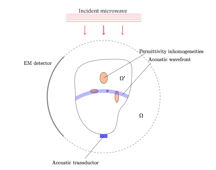
Figure 1. The acousto-electromagnetic tomography experiment.

We now briefly describe how to measure the internal data in the hybrid problem under consideration. The reader is referred to [14] for full details.

Let $\Omega\subset\mathbb{R}^{d}$ be a bounded and smooth domain, for $d=2$ or $d=3$ and $q\in L^{\infty}(\Omega;\mathbb{R})\cap H^{1}(\Omega;\mathbb{R})$ be the electric permittivity of the medium. We assume that $q$ is known and constant near the boundary $\partial\Omega$, namely $q=1$ in $\Omega\setminus\Omega^{\prime}$, for some $\Omega^{\prime}\Subset\Omega$. More precisely, suppose that $q\in Q$, where for some $\Lambda>0$

(2) $$Q:=\{q\in H^{1}(\Omega;\mathbb{R}):\Lambda^{-1}\leq q\leq\Lambda\text{ in $\Omega$, $\left\|q\right\|_{H^{1}(\Omega)}\leq\Lambda$\ and $q=1\;$in $\Omega\setminus\Omega^{\prime}$}\}.$$

In this paper, we model electromagnetic propagation in $\Omega$ at frequency $\omega\in\mathcal{A}=[K_{min},K_{max}]\subset\mathbb{R}_{+}$ by (1). The boundary value problem model allows us to consider arbitrary $q$ beyond the Born approximation, and so it is used here instead of the free propagation model, which was originally considered in [14]. Problem (1) admits a unique solution $u_{\omega}\in H^{1}(\Omega;\mathbb{C})$ for a fixed boundary condition $\varphi\in H^{1}(\Omega;\mathbb{C})$ (see Lemma 3).

Let us discuss how microwaves are combined with acoustic waves. A short acoustic wave creates a displacement field $v$ in $\Omega$ (whose support is the blue area in Figure 1), which we suppose continuous and bijective. Then, the permittivity distribution $q$ becomes $q_{v}$ defined by

$$q_{v}(x+v(x))=q(x),\qquad x\in\Omega,$$

and the complex amplitude $u_{\omega}^{v}$ of the electric wave in the perturbed medium satisfies

(3) $$\Delta u_{\omega}^{v}+\omega^{2}q_{v}u_{\omega}^{v}=0\text{ in }\Omega.$$

Using (1) and (3), for $v$ small enough we obtain the cross-correlation formula

$$\int_{\partial\Omega}(\frac{\partial u_{\omega}}{\partial n}\overline{u_{\omega}^{v}}-\frac{\partial\overline{v}}{\partial n}u_{\omega})\,d\sigma=\omega^{2}\int_{\Omega}(q_{v}-q)u_{\omega}\overline{u_{\omega}^{v}}\,dx\approx\omega^{2}\int_{\Omega}|u_{\omega}|^{2}\nabla q\cdot v\,dx,$$

By boundary measurements, the left hand side of this equality is known. Thus, we have measurements of the form

$$\int_{\Omega}|u_{\omega}|^{2}\nabla q\cdot v\,dx,$$

for all perturbations $v$. It is shown in [14, 13] that choosing radial displacements $v$ allows to recover the gradient part of $|u_{\omega}|^{2}\nabla q$ by using the inversion for the spherical mean Radon transform. Namely, writing the Helmholtz decomposition of $|u_{\omega}|^{2}\nabla q$

$$|u_{\omega}|^{2}\nabla q=\nabla\psi_{\omega}+{\rm curl}\Phi_{\omega},$$

for $\psi_{\omega}\in H^{1}(\Omega;\mathbb{R})$ and $\Phi_{\omega}\in H^{1}(\Omega;\mathbb{R}^{2d-3})$, the potential $\psi_{\omega}$ can be measured. Moreover, $\psi_{\omega}$ is the unique solution to [19, Chapter I, Theorem 3.2 and Corollary 3.4]

(4) $$\left\{\begin{array}[]{l}\Delta\psi_{\omega}={\rm div}(|u_{\omega}|^{2}\nabla q)\qquad\text{in }\Omega,\\ \frac{\partial\psi_{\omega}}{\partial\nu}=0\qquad\text{on }\partial\Omega,\\ \int_{\Omega}\psi_{\omega}\,dx=0.\end{array}\right.$$

In this paper, we assume that the inversion of the spherical mean Radon transform has been performed and that we have access to $\psi_{\omega}$. In the following, we shall deal with the second step of this hybrid imaging problem: recovering the map $q$ from the knowledge of $\psi_{\omega}$.

2.2. The Landweber Iteration

Let $q^{*}$ be the real permittivity with corresponding measurements $\psi_{\omega}^{*}$. Let $K\subset\mathcal{A}$ be a finite set of admissible frequencies for which we have the measurements $\psi_{\omega}^{*}$, $\omega\in K$. The set $K$ will be determined later. Let us denote the error map by

(5) $$F_{\omega}\colon Q\to H_{\nu}^{1}(\Omega;\mathbb{R}),\qquad q\mapsto\psi_{\omega}(q)-\psi_{\omega}^{*},$$

where $\psi_{\omega}(q)$ is the unique solution to (4), and $H_{\nu}^{1}(\Omega;\mathbb{R})=\{u\in H^{1}(\Omega;\mathbb{R}):\frac{\partial u}{\partial\nu}=0\text{ on $\partial\Omega$}\}$.

A natural approach to recover the real conductivity is to minimize the discrepancy functional $J$ defined as

(6) $$J(q)=\frac{1}{2}\sum_{\omega\in K}\int_{\Omega}|F_{\omega}(q)|^{2}dx,\qquad q\in Q.$$

The gradient descent method can be employed to minimize $J$. At each iteration we compute

$$q_{n+1}=T\left(q_{n}-hDJ[q_{n}]\right),$$

where $h>0$ is the step size and $T\colon H^{1}(\Omega;\mathbb{R})\to Q$ is the Hilbert projection onto the convex closed set $Q$, which guarantees that at each iteration $q_{n}$ belongs to the admissible set $Q$. Since $DJ[q]=\sum_{\omega}DF_{\omega}[q]^{*}(F_{\omega}(q))$, this algorithm is equivalent to the Landweber scheme [20] given by

(7) $$q_{n+1}=T\Bigl{(}q_{n}-h\sum_{\omega\in K}DF_{\omega}(q_{n})^{*}(F_{\omega}(q_{n}))\Bigr{)}.$$

(For the Fréchet differentiability of the map $F_{\omega}$, see Lemma 5.)

The main result of this paper states that the Landweber scheme defined above converges to the real unknown $q^{*}$, provided that $K$ is suitably chosen and that $h$ and $\left\|q_{0}-q^{*}\right\|_{H^{1}(\Omega)}$ are small enough. The most natural choice for the set of frequencies $K$ is as a uniform sample of $\mathcal{A}$, namely let

$$K^{(m)}=\{\omega_{1}^{(m)},\dots,\omega_{m}^{(m)}\},\qquad\omega_{i}^{(m)}=K_{min}+\frac{(i-1)}{(m-1)}(K_{max}-K_{min}).$$

Theorem 1.

Set $\varphi=1$. There exist $C>0$ and $m\in\mathbb{N}^{*}$ depending only on $\Omega$, $\Lambda$ and $\mathcal{A}$ such that for any $q\in Q$ and $\rho\in H_{\nu}^{1}(\Omega;\mathbb{R})$

(8) $$\sum_{\omega\in K^{(m)}}\left\|DF_{\omega}[q](\rho)\right\|{}_{H^{1}(\Omega;\mathbb{R})}d\omega\geq C\left\|\rho\right\|{}_{H^{1}(\Omega;\mathbb{R})}.$$

As a consequence, the sequence defined in (7) converges to $q^{*}$ provided that $h$ and $\left\|q_{0}-q^{*}\right\|_{H^{1}(\Omega)}$ are small enough.

The proof of this theorem is presented in Section 3. In view of the results in [20, 9], the convergence of the Landweber iteration follows from the Lipschitz continuity of $F_{\omega}$ and from inequality (8). The Lipschitz continuity of $F_{\omega}$ is a simple consequence of the elliptic theory.

On the other hand, the lower bound given in (8) is non-trivial, since it represents the uniqueness and stability of the multi-frequency linearized inverse problem

$$(DF_{\omega}[q](\rho))_{\omega\in K^{(m)}}\longmapsto\rho.$$

As it has been discussed in the Introduction, the kernels of the operators $\rho\mapsto DF_{\omega}[q](\rho)$ “move” as $\omega$ changes. More precisely, the intersection of the kernels corresponding to the a priori determined finite set of frequencies $K^{(m)}$ is empty. Moreover, the argument automatically gives an a priori constant $C$ in (8).

The multi-frequency method is based on the analytic dependence of the problem with respect to the frequency $\omega$, and on the fact that in $\omega=0$ the problem is well posed. Indeed, when $\omega\to 0$ it is easy to see that $u_{\omega}\to 1$ in (1), so that $u_{0}=1$. Thus, looking at (4), the measurement datum $\psi_{0}$ is nothing else than $q^{*}$ (up to a constant). Therefore, $q^{*}$ could be easily determined when $\omega=0$ since $q^{*}$ is known on the boundary $\partial\Omega$. As we show in the following section, the analyticity of the problem with respect to $\omega$ allows to “transfer” this property to the desired range of frequencies $\mathcal{A}$.

3. Convergence of the Landweber Iteration

In order to use the well-posedness of the problem in $\omega=0$ we shall need the following result on quantitative unique continuation for vector-valued holomorphic functions.

Lemma 2.

Let $V$ be a complex Banach space, $\mathcal{A}=[K_{min},K_{max}]\subset\mathbb{R}_{+}$, $C_{0},D>0$ and $g\colon B(0,K_{max})\to V$ be holomorphic such that $\left\|g(0)\right\|\geq C_{0}$ and

$$\sup_{\omega\in B(0,K_{max})}\left\|g(\omega)\right\|\leq D.$$

Then there exists $\omega\in\mathcal{A}$ such that

$$\left\|g(\omega)\right\|\geq C$$

for some $C>0$ depending only on $\mathcal{A}$, $C_{0}$ and $D$.

Proof.

By contradiction, assume that there exists a sequence of holomorphic functions $g_{n}\colon B(0,K_{max})\to V$ such that $\left\|g_{n}(0)\right\|\geq C_{0}$, $\sup_{\omega\in B(0,K_{max})}\left\|g_{n}(\omega)\right\|\leq D$ and $\max_{\omega\in\mathcal{A}}\left\|g_{n}(\omega)\right\|\to 0$. By Hahn Banach theorem, for any $n$ there exists $T_{n}\in V^{\prime}$ such that $\left\|T_{n}\right\|\leq 1$ and $T_{n}(g_{n}(0))=\left\|g_{n}(0)\right\|$. Set $f_{n}:=T_{n}\circ g_{n}\colon B(0,K_{max})\to\mathbb{C}$. Thus $(f_{n})$ is a family of complex-valued uniformly bounded holomorphic functions, since

$$\left|f_{n}(\omega)\right|\leq\left\|T_{n}\right\|\left\|g_{n}(\omega)\right\|\leq D,\qquad\omega\in B(0,K_{max}).$$

As a consequence, by standard complex analysis, there exists a holomorphic function $f\colon B(0,K_{max})\to\mathbb{C}$ such that $f_{n}\to f$ uniformly. We readily observe that for any $\omega\in\mathcal{A}$ there holds

$$\left|f(\omega)\right|=\lim_{n}\left|f_{n}(\omega)\right|\leq\lim_{n}\left\|T_{n}\right\|\left\|g_{n}(\omega)\right\|=0,$$

since $\max_{\omega\in\mathcal{A}}\left\|g_{n}(\omega)\right\|\to 0$. By the unique continuation theorem $f(0)=0$. On the other hand, as $T_{n}(g_{n}(0))=\left\|g_{n}(0)\right\|$,

$$f(0)=\lim_{n}f_{n}(0)=\lim\left\|g_{n}(0)\right\|\geq C_{0}>0,$$

which yields a contradiction. ∎

In view of (8), we need to study the Fréchet differentiability of the map $F_{\omega}$ and characterize its derivative. Before doing this, we study the well-posedness of (1). The result is classical; for a proof, see [24, Section 8.1].

Lemma 3.

Let $\Omega\subset\mathbb{R}^{d}$ be a bounded and smooth domain for $d=2,3$, $\omega\in B(0,K_{max})$ and $q\in Q$. For any $f\in L^{2}(\Omega;\mathbb{C})$ and $\varphi\in H^{1}(\Omega;\mathbb{C})$ the problem

(9) $$\left\{\begin{array}[]{l}\Delta u+\omega^{2}qu=\omega f\qquad\text{in }\Omega,\\ \frac{\partial u}{\partial\nu}-i\omega u=-i\omega\varphi\qquad\text{on }\partial\Omega,\end{array}\right.$$

augmented with the condition

(10) $$\int_{\partial\Omega}u\,d\sigma=\int_{\partial\Omega}\varphi\,d\sigma-i\int_{\Omega}f\,dx$$

if $\omega=0$ admits a unique solution $u\in H^{2}(\Omega;\mathbb{C})$. Moreover

$$\left\|u\right\|_{H^{2}(\Omega;\mathbb{C})}\leq C\bigl{(}\left\|f\right\|_{L^{2}(\Omega;\mathbb{C})}+\left\|\varphi\right\|_{H^{1}(\Omega;\mathbb{C})}\bigr{)}$$

for some $C>0$ depending only on $\Omega$, $\Lambda$ and $K_{max}$.

Since for $\omega=0$ the solution to (9) is unique up to a constant, condition (10) is needed to have uniqueness. Even though it may seem mysterious, this condition is natural in order to ensure continuity of $u$ with respect to $\omega$. Indeed an integration by parts gives

$$\omega\int_{\Omega}f\,dx=\int_{\partial\Omega}\frac{\partial u}{\partial\nu}\,d\sigma+\omega^{2}\int_{\Omega}qu\,dx=i\omega\int_{\partial\Omega}(u-\varphi)\,d\sigma+\omega^{2}\int_{\Omega}qu\,dx,$$

whence for $\omega\neq 0$ we obtain

$$\int_{\partial\Omega}u\,d\sigma=\int_{\partial\Omega}\varphi\,d\sigma-i\int_{\Omega}f\,dx+\omega i\int_{\Omega}qu\,dx,$$

and so for $\omega=0$ we are left with (10). The above condition is a consequence of (9) for $\omega\neq 0$, but needs to be added in the case $\omega=0$ to guarantee uniqueness.

Let us go back to (1). Fix $\varphi\in H^{1}(\Omega;\mathbb{C})$ and $\omega\in B(0,K_{max})$. By Lemma 3 the problem

(11) $$\left\{\begin{array}[]{l}\Delta u_{\omega}+\omega^{2}qu_{\omega}=0\text{ in }\Omega,\\ \frac{\partial u_{\omega}}{\partial n}-i\omega u_{\omega}=-i\omega\varphi\text{ on }\partial\Omega,\end{array}\right.$$

together with condition

(12) $$\int_{\partial\Omega}u_{\omega}\,d\sigma=\int_{\partial\Omega}\varphi\,d\sigma+\omega i\int_{\Omega}qu_{\omega}\,dx$$

admits a unique solution $u_{\omega}\in H^{2}(\Omega;\mathbb{C})$ such that

(13) $$\left\|u_{\omega}\right\|_{H^{2}(\Omega;\mathbb{C})}\leq C\left\|\varphi\right\|_{H^{1}(\Omega;\mathbb{C})}$$

for some $C>0$ depending only on $\Omega$, $\Lambda$ and $K_{max}$. As above, (12) guarantees uniqueness and continuity in $\omega=0$ and is implicit in (11) if $\omega\neq 0$.

Next, we study the dependence of $u_{\omega}$ on $\omega$.

Lemma 4.

Let $\Omega\subset\mathbb{R}^{d}$ be a bounded and smooth domain for $d=2,3$, $q\in Q$ and $\varphi\in H^{1}(\Omega;\mathbb{C})$. The map

$$\mathcal{F}(q)\colon B(0,K_{max})\longrightarrow H^{2}(\Omega;\mathbb{C}),\qquad\omega\longmapsto u_{\omega}$$

is holomorphic. Moreover, the derivative $\partial_{\omega}u_{\omega}\in H^{2}(\Omega;\mathbb{C})$ is the unique solution to

(14) $$\left\{\begin{array}[]{l}\Delta\partial_{\omega}u_{\omega}+\omega^{2}q\partial_{\omega}u_{\omega}=-2\omega qu_{\omega}\text{ in }\Omega,\\ \frac{\partial(\partial_{\omega}u_{\omega})}{\partial\nu}-i\omega\partial_{\omega}u_{\omega}=iu_{\omega}-i\varphi\text{ on }\partial\Omega,\end{array}\right.$$

together with condition

(15) $$\int_{\partial\Omega}\partial_{\omega}u_{\omega}\,d\sigma=\omega i\int_{\Omega}q\partial_{\omega}u_{\omega}\,dx+i\int_{\Omega}qu_{\omega}\,dx,$$

and satisfies

$$\left\|\partial_{\omega}u_{\omega}\right\|_{H^{2}(\Omega;\mathbb{C})}\leq C\left\|\varphi\right\|_{H^{1}(\Omega;\mathbb{C})}$$

for some $C>0$ depending only on $\Omega$, $\Lambda$ and $K_{max}$.

Proof.

The proof of this result is completely analogous to the ones given in [1, 2, 9] in similar situations. Here only a sketch will be presented.

Fix $\omega\in B(0,K_{max})$: we shall prove that $\mathcal{F}(q)$ is holomorphic in $\omega$ and that the derivative is $\partial_{\omega}u_{\omega}$, i.e., the unique solution to (14)-(15). For $h\in\mathbb{C}$ let $v_{h}=(u_{\omega+h}-u_{\omega})/h$. We need to prove that $v_{h}\to\partial_{\omega}u_{\omega}$ in $H^{2}(\Omega)$ as $h\to 0$. Suppose first $\omega\neq 0$. A direct calculation shows that

$$\left\{\begin{array}[]{l}\Delta v_{h}+\omega^{2}qv_{h}=-2\omega qu_{\omega+h}-hqu_{\omega+h}\text{ in }\Omega,\\ \frac{\partial v_{h}}{\partial\nu}-i\omega v_{h}=i(u_{\omega+h}-\varphi)\text{ on }\partial\Omega.\end{array}\right.$$

Arguing as in Lemma 3, we obtain $u_{\omega+h}\to u_{\omega}$ as $h\to 0$ in $H^{2}(\Omega)$, whence $v_{h}\to\partial_{\omega}u_{\omega}$ in $H^{2}(\Omega)$, as desired.

When $\omega=0$, the above system must be augmented with the condition

$$\int_{\partial\Omega}v_{h}\,d\sigma=i\int_{\Omega}qu_{0}\,dx,$$

which is a simple consequence of (12), and the result follows. ∎

We now study the Fréchet differentiability of the map $F_{\omega}$ defined in (5). The proof of this result is trivial, and the details are left to the reader.

Lemma 5.

Let $\Omega\subset\mathbb{R}^{d}$ be a bounded and smooth domain for $d=2,3$, $q\in Q$, $\omega\in B(0,K_{max})$ and $\varphi\in H^{1}(\Omega;\mathbb{C})$. The map $F_{\omega}$ is Fréchet differentiable and for $\rho\in H_{\nu}^{1}(\Omega;\mathbb{R})$, the derivative $\xi_{\omega}(\rho):=DF_{\omega}[q](\rho)$ is the unique solution to the problem

$$\left\{\begin{array}[]{l}\Delta\xi_{\omega}(\rho)={\rm div}\left(|u_{\omega}|^{2}\nabla\rho+(\overline{u}_{\omega}v_{\omega}(\rho)+u_{\omega}\overline{v}_{\omega}(\rho))\nabla q\right)\text{ in }\Omega,\\ \frac{\partial\xi_{\omega}(\rho)}{\partial\nu}=0\text{ on }\partial\Omega,\\ \int_{\Omega}\xi_{\omega}(\rho)\,dx=0,\end{array}\right.$$

where $v_{\omega}(\rho)\in H^{2}(\Omega;\mathbb{C})$ is the unique solution to

(16) $$\left\{\begin{array}[]{l}\Delta v_{\omega}(\rho)+\omega^{2}qv_{\omega}(\rho)=-\omega^{2}\rho\,u_{\omega}\text{ in }\Omega,\\ \frac{\partial v_{\omega}(\rho)}{\partial\nu}-i\omega v_{\omega}(\rho)=0\text{ on }\partial\Omega,\end{array}\right.$$

together with $\int_{\partial\Omega}v_{0}(\rho)\,d\sigma=0$ if $\omega=0$. In particular, $F_{\omega}$ is Lipschitz continuous, namely

$$\left\|\xi_{\omega}(\rho)\right\|_{H^{1}(\Omega;\mathbb{R})}\leq C(\Omega,\Lambda,K_{max},\left\|\varphi\right\|_{H^{1}(\Omega;\mathbb{C})})\left\|\rho\right\|_{H^{1}(\Omega;\mathbb{R})}.$$

The main step in the proof of Theorem 1 is inequality (8), which we now prove. The argument in the proof clarifies the multi-frequency method illustrated in the previous section. The proof is structured as the proof of [3, Theorem 1].

Proposition 6.

Set $\varphi=1$. There exist $C>0$ and $m\in\mathbb{N}^{*}$ depending on $\Omega$, $\Lambda$ and $\mathcal{A}$ such that for any $q\in Q$ and $\rho\in H_{\nu}^{1}(\Omega;\mathbb{R})$

$$\sum_{\omega\in K^{(m)}}\left\|DF_{\omega}[q](\rho)\right\|{}_{H^{1}(\Omega;\mathbb{R})}d\omega\geq C\left\|\rho\right\|{}_{H^{1}(\Omega;\mathbb{R})}.$$

Proof.

In the proof, several positive constants depending only on $\Omega$, $\Lambda$ and $\mathcal{A}$ will be denoted by $C$ or $Z$.

Fix $q\in Q$. For $\rho\in H_{\nu}^{1}(\Omega;\mathbb{R})$ such that $\left\|\rho\right\|_{H^{1}(\Omega;\mathbb{R})}=1$ define the map

$$g_{\rho}(\omega)={\rm div}\left(u_{\omega}\overline{u}_{\overline{\omega}}\nabla\rho+(\overline{u}_{\overline{\omega}}v_{\omega}(\rho)+u_{\omega}\overline{v}_{\overline{\omega}}(\rho))\nabla q\right),\qquad\omega\in B(0,K_{max}).$$

Hence $g_{\rho}\colon B(0,K_{max})\to H_{\nu}^{1}(\Omega;\mathbb{C})^{\prime}$ is holomorphic. We shall apply Lemma 2 to $g_{\rho}$, and so we now verify the hypotheses.

Since $\varphi=1$, by (11)-(12) we have $u_{0}=1$ and by (16) we have $v_{0}(\rho)=0$, whence $g_{\rho}(0)={\rm div}(\nabla\rho)$. Since $\frac{\partial\rho}{\partial\nu}=0$ on $\partial\Omega$ there holds

$$\left\|g_{\rho}(0)\right\|_{H_{\nu}^{1}(\Omega;\mathbb{C})^{\prime}}=\left\|{\rm div}(\nabla\rho)\right\|_{H_{\nu}^{1}(\Omega;\mathbb{C})^{\prime}}\geq C\left\|\nabla\rho\right\|_{L^{2}(\Omega)}\geq C>0,$$

since $\left\|\rho\right\|_{H^{1}(\Omega;\mathbb{R})}=1$. For $\omega\in B(0,K_{max})$ we readily derive

$$\begin{split}\left\|g_{\rho}(\omega)\right\|_{H_{\nu}^{1}(\Omega;\mathbb{C})^{\prime}}&\leq C\left\|u_{\omega}\overline{u}_{\overline{\omega}}\nabla\rho+(\overline{u}_{\overline{\omega}}v_{\omega}(\rho)+u_{\omega}\overline{v}_{\overline{\omega}}(\rho))\nabla q\right\|_{L^{2}(\Omega)}\\ &\leq C\left(\left\|\rho\right\|_{H^{1}(\Omega)}+\left\|q\right\|_{H^{1}(\Omega)}\right)\\ &\leq C,\end{split}$$

where the second inequality follows from (13), Lemma 3 applied to $v_{\omega}(\rho)$ and the Sobolev embedding $H^{2}\hookrightarrow L^{\infty}$. Therefore, by Lemma 2 there exists $\omega_{\rho}\in\mathcal{A}$ such that

(17) $$\left\|g_{\rho}(\omega_{\rho})\right\|_{H_{\nu}^{1}(\Omega;\mathbb{C})^{\prime}}\geq C.$$

Consider now for $\omega\in B(0,K_{max})$

$$g_{\rho}^{\prime}(\omega)={\rm div}\left((u^{\prime}_{\omega}\overline{u}_{\overline{\omega}}+u{}_{\omega}\overline{u^{\prime}}_{\overline{\omega}})\nabla\rho+(\overline{u^{\prime}}_{\overline{\omega}}v_{\omega}(\rho)+\overline{u}_{\overline{\omega}}v^{\prime}_{\omega}(\rho)+u^{\prime}_{\omega}\overline{v}_{\overline{\omega}}(\rho)+u_{\omega}\overline{v^{\prime}}_{\overline{\omega}}(\rho))\nabla q\right)$$

where for simplicity the partial derivative $\partial_{\omega}$ is replaced by ^′. Arguing as before, and using Lemma 4 we obtain

$$\left\|g^{\prime}_{\rho}(\omega)\right\|_{H_{\nu}^{1}(\Omega;\mathbb{C})^{\prime}}\leq C,\qquad\omega\in B(0,K_{max}).$$

As a consequence, by (17) we obtain

(18) $$\left\|g_{\rho}(\omega)\right\|_{H_{\nu}^{1}(\Omega;\mathbb{C})^{\prime}}\geq C,\qquad\omega\in[\omega_{\rho}-Z,\omega_{\rho}+Z]\cap\mathcal{A}.$$

Since $\mathcal{A}=[K_{min},K_{max}]$ there exists $P=P(Z,\mathcal{A})\in\mathbb{N}$ such that

(19) $$\mathcal{A}\subseteq\bigcup_{p=1}^{P}I_{p},\qquad I_{p}=[K_{min}+(p-1)Z,K_{min}+pZ].$$

Choose now $m\in\mathbb{N}^{*}$ big enough so that for every $p=1,\dots,P$ there exists $i_{p}=1,\dots,m$ such that $\omega(p):=\omega_{i_{p}}^{(m)}\in I_{p}$ (recall that $\omega_{i}^{(m)}=K_{min}+\frac{(i-1)}{(m-1)}(K_{max}-K_{min})$). Note that $m$ depends only on $Z$ and $\left|\mathcal{A}\right|$.

Since $\left|[\omega_{\rho}-Z,\omega_{\rho}+Z]\right|=2Z$ and $\left|I_{p}\right|=Z$, in view of (19) there exists $p_{\rho}=1,\dots,P$ such that $I_{p_{\rho}}\subseteq[\omega_{\rho}-Z,\omega_{\rho}+Z]$. Therefore $\omega(p_{\rho})\in[\omega_{\rho}-Z,\omega_{\rho}+Z]\cap\mathcal{A}$, whence by (18) there holds $\left\|g_{\rho}(\omega(p_{\rho}))\right\|_{H_{\nu}^{1}(\Omega;\mathbb{C})^{\prime}}\geq C$. Since $\omega(p_{\rho})\in\mathbb{R}$ this implies

$$\left\|{\rm div}\left(|u_{\omega(p_{\rho})}|^{2}\nabla\rho+(\overline{u}_{\omega(p_{\rho})}v_{\omega}(\rho)+u_{\omega}\overline{v}_{\omega(p_{\rho})}(\rho))\nabla q\right)\right\|_{H_{\nu}^{1}(\Omega;\mathbb{C})^{\prime}}\geq C,$$

which by Lemma 5 yields $\left\|\Delta\xi_{\omega(p_{\rho})}(\rho)\right\|_{H_{\nu}^{1}(\Omega;\mathbb{C})^{\prime}}\geq C$. Hence, since $\frac{\partial\xi_{\omega(p_{\rho})}(\rho)}{\partial\nu}=0$ on $\partial\Omega$, there holds $\left\|\xi_{\omega(p_{\rho})}(\rho)\right\|_{H^{1}(\Omega)}\geq C$. Thus, since $\omega(p_{\rho})\in K^{(m)}$

$$\sum_{\omega\in K^{(m)}}\left\|\xi_{\omega}(\rho)\right\|_{H^{1}(\Omega)}\geq C.$$

We have proved this inequality only for $\rho\in H_{\nu}^{1}(\Omega;\mathbb{R})$ with unitary norm. By using the linearity of $\xi_{\omega}(\rho)$ with respect to $\rho$ we immediately obtain

$$\sum_{\omega\in K^{(m)}}\left\|\xi_{\omega}(\rho)\right\|_{H^{1}(\Omega)}\geq C\left\|\rho\right\|_{H^{1}(\Omega)},\qquad\rho\in H_{\nu}^{1}(\Omega;\mathbb{R}),$$

as desired. ∎

We are now ready to prove Theorem 1.

Proof of Theorem 1.

Inequality (8) follows from Proposition 6. Moreover, $F_{\omega}$ is Lipschitz continuous by Lemma 5. Therefore, the convergence of the Landweber iteration is a consequence of the results in [9, 20], provided that $\left\|q_{0}-q^{*}\right\|_{H^{1}(\Omega)}$ and $h$ are small enough. ∎

4. Numerical Results

In this section we present some numerical results. Let $\Omega$ be the unit square $[0,1]\times[0,1]$. We set the mesh size to be $0.01$. A phantom image is used for the true permittivity distribution $q^{*}$ (see Figure 2). According to Theorem 1 we set the Robin boundary condition to be a constant function $\varphi=1$. Let $K$ be the set of frequencies for which we have measurements $\psi_{\omega}^{*}$, $\omega\in K$. As discussed in $\S$ 2.2, we minimize the functional $J$ in (6) with the Landweber iteration scheme given in (7). The initial guess is $q_{0}=1$.

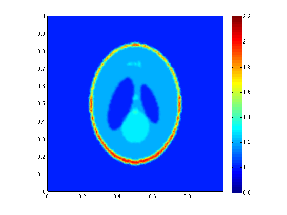
Figure 2. The true permittivity distribution $q^{*}$.

We start with the imaging problem at a single frequency. In Figure 3 we display the findings for the case $K=\{3\}$. Figure 3a shows the reconstructed distribution after 100 iterations. Figure 3b shows the relative error as a function of the number of iterations. This suggests the convergence of the iterative algorithm, even though the algorithm is proved to be convergent only in the multi-frequency case. It is possible that for small frequencies $\omega$ (with respect to the domain size) we are still in the coercive case, i.e. the kernel $R_{\omega}$ of $\rho\mapsto DF_{\omega}[q](\rho)$ is trivial and a single frequency is sufficient.

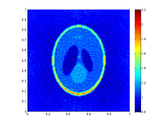
(a) Reconstructed distribution after 100 iterations.

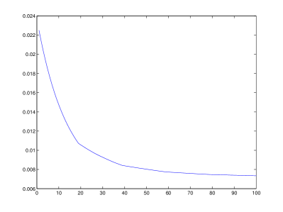
(b) Relative error depending on the number of iterations.

Figure 3. Reconstruction of $q$ for the set of frequencies $K=\{3\}$.

However, this does not work at higher frequencies (with respect to the domain size). Figure 4 shows some reconstructed maps for $\omega=10$, $\omega=15$ and $\omega=20$, which suggest that the algorithm may not converge numerically for high frequencies. In each case, there are areas that remain invisible. This may be an indication that $R_{\omega}\neq\{0\}$ for these values of the frequency.

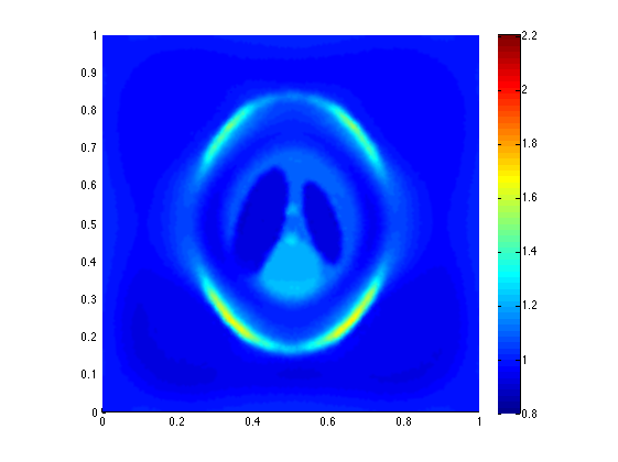
(a) $K=\{10\}$

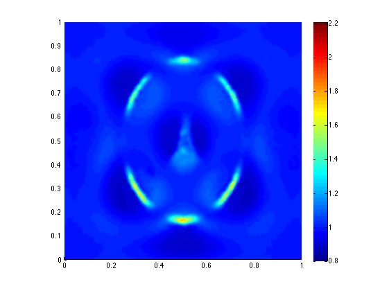
(b) $K=\{15\}$

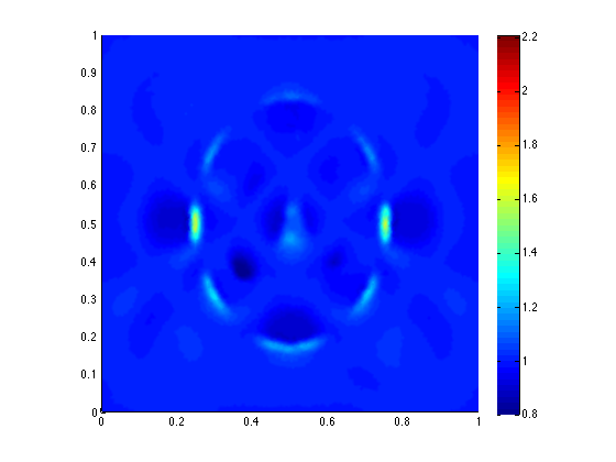
(c) $K=\{20\}$

Figure 4. Reconstruction of $q$ for higher frequencies.

The invisible areas in Figure 4 are different for different frequencies, and so combining these measurements may give a satisfactory reconstruction. More precisely, according to Theorem 1, by using multiple frequencies it is possible to make the problem injective, namely $\cap_{\omega}R_{\omega}=\{0\}$, since the kernels $R_{\omega}$ change as $\omega$ varies. Figure 5 shows the results for the case $K=\left\{10,15,20\right\}$. (According to the notation introduced in Section 2, this choice of frequencies corresponds to $\mathcal{A}=[10,20]$ and $m=3$.) These findings suggest the convergence of the multi-frequency Landweber iteration, even though it was not convergent in each single-frequency case. Since we chose higher frequencies, the convergence is slower.

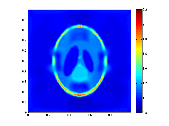
(a) Reconstructed distribution after 200 iterations.

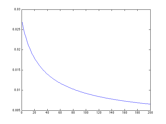
(b) Relative error depending on the number of iterations.

Figure 5. Reconstruction of $q$ for $K=\{10,15,20\}$.

5. Concluding Remarks

In this paper, we proved that the Landweber scheme in acousto-electromagnetic tomography converges to the true solution provided that multi-frequency measurements are used. We illustrated this result with several numerical examples. It would be challenging to estimate the robustness of the proposed algorithm with respect to random fluctuations in the electromagnetic parameters. This will be the subject of a forthcoming work.

References

• [1] Giovanni S. Alberti. On multiple frequency power density measurements. Inverse Problems, 29(11):115007, 25, 2013. doi:10.1088/0266-5611/29/11/115007.
• [2] Giovanni S. Alberti. On multiple frequency power density measurements II. The full Maxwell’s equations. ArXiv e-prints, November 2013. arXiv:1311.7603.
• [3] Giovanni S. Alberti. Enforcing local non-zero constraints in PDEs and applications to hybrid imaging problems. ArXiv e-prints, June 2014. arXiv:1406.3248.
• [4] Giovanni S. Alberti. On local constraints and regularity of PDE in electromagnetics. Applications to hybrid imaging inverse problems. PhD thesis, University of Oxford, 2014. Available from: http://ora.ox.ac.uk/objects/uuid:1b30b3b7-29b1-410d-ae30-bd0a87c9720b.
• [5] Giovanni S. Alberti and Yves Capdeboscq. A propos de certains problèmes inverses hybrides. In Seminaire: Equations aux Dérivées Partielles. 2013–2014, Sémin. Équ. Dériv. Partielles, page Exp. No. II. École Polytech., Palaiseau, 2014. Available from: http://slsedp.cedram.org/cedram-bin/article/SLSEDP_2013-2014____A2_0.pd%f.
• [6] Giovanni S. Alberti and Yves Capdeboscq. Lectures on elliptic methods for hybrid inverse problems. In preparation.
• [7] H. Ammari, E. Bonnetier, Y. Capdeboscq, M. Tanter, and M. Fink. Electrical impedance tomography by elastic deformation. SIAM J. Appl. Math., 68(6):1557–1573, 2008. doi:10.1137/070686408.
• [8] H. Ammari, Y. Capdeboscq, F. de Gournay, A. Rozanova-Pierrat, and F. Triki. Microwave imaging by elastic deformation. SIAM J. Appl. Math., 71(6):2112–2130, 2011. doi:10.1137/110828241.
• [9] H. Ammari, L. Giovangigli, L. Hoang Nguyen, and J.-K. Seo. Admittivity imaging from multi-frequency micro-electrical impedance tomography. ArXiv e-prints, March 2014. arXiv:1403.5708.
• [10] H. Ammari and H. Kang. Expansion methods. In Handbook of Mathematical Methods in Imaging, pages 447–499. Springer, New York, 2011.
• [11] H. Ammari, A. Waters, and H. Zhang. Stability Analysis for Magnetic Resonance Elastography. ArXiv e-prints, September 2014. arXiv:1409.5138.
• [12] Habib Ammari. An introduction to mathematics of emerging biomedical imaging, volume 62. Springer, 2008.
• [13] Habib Ammari, Emmanuel Bossy, Josselin Garnier, Loc Hoang Nguyen, and Laurent Seppecher. A reconstruction algorithm for ultrasound-modulated diffuse optical tomography. Proc. Amer. Math. Soc., 142(9):3221–3236, 2014. doi:10.1090/S0002-9939-2014-12090-9.
• [14] Habib Ammari, Emmanuel Bossy, Josselin Garnier, and Laurent Seppecher. Acousto-electromagnetic tomography. SIAM J. Appl. Math., 72(5):1592–1617, 2012. doi:10.1137/120863654.
• [15] Guillaume Bal. Hybrid inverse problems and internal functionals. In G. Uhlmann, editor, Inverse problems and applications: inside out. II, volume 60 of Math. Sci. Res. Inst. Publ., pages 325–368. Cambridge Univ. Press, Cambridge, 2013.
• [16] Guillaume Bal. Hybrid inverse problems and redundant systems of partial differential equations. In P. Stefanov, A. Vasy, and M. Zworski, editors, Inverse Problems and Applications, volume 615 of Contemporary Mathematics. American Mathematical Society, 2014.
• [17] Guillaume Bal and Shari Moskow. Local inversions in ultrasound-modulated optical tomography. Inverse Problems, 30(2):025005, 17, 2014. doi:10.1088/0266-5611/30/2/025005.
• [18] Guillaume Bal and John C. Schotland. Ultrasound-modulated bioluminescence tomography. Phys. Rev. E, 89:031201, Mar 2014. doi:10.1103/PhysRevE.89.031201.
• [19] Vivette Girault and Pierre-Arnaud Raviart. Finite element methods for Navier-Stokes equations, volume 5 of Springer Series in Computational Mathematics. Springer-Verlag, Berlin, 1986. Theory and algorithms. doi:10.1007/978-3-642-61623-5.
• [20] Martin Hanke, Andreas Neubauer, and Otmar Scherzer. A convergence analysis of the Landweber iteration for nonlinear ill-posed problems. Numer. Math., 72(1):21–37, 1995. doi:10.1007/s002110050158.
• [21] P. Kuchment. Mathematics of Hybrid Imaging: A Brief Review. In Irene Sabadini and Daniele C Struppa, editors, The Mathematical Legacy of Leon Ehrenpreis, volume 16 of Springer Proceedings in Mathematics, pages 183–208. Springer Milan, 2012. doi:10.1007/978-88-470-1947-8_12.
• [22] P. Kuchment and D. Steinhauer. Stabilizing inverse problems by internal data. II. Non-local internal data and generic linearized uniqueness. ArXiv e-prints, July 2014. arXiv:1407.0763.
• [23] Peter Kuchment and Dustin Steinhauer. Stabilizing inverse problems by internal data. Inverse Problems, 28(8):084007, 20, 2012. doi:10.1088/0266-5611/28/8/084007.
• [24] Jens Markus Melenk. On generalized finite element methods. PhD thesis, The University of Maryland, 1995. Available from: http://www.math.tuwien.ac.at/~melenk/publications/diss.ps.gz.
• [25] Carlos Montalto and Plamen Stefanov. Stability of coupled-physics inverse problems with one internal measurement. Inverse Problems, 29(12):125004, 13, 2013. doi:10.1088/0266-5611/29/12/125004.
• [26] T. Widlak and O. Scherzer. Stability in the linearized problem of quantitative elastography. ArXiv e-prints, June 2014. arXiv:1406.0291.