Gegenbauer-Chebyshev Integrals and Radon Transforms

Abstract.

We suggest new modifications of Helgason’s support theorems and descriptions of the kernels for several projectively equivalent transforms of integral geometry. The paper deals with the hyperplane Radon transform and its dual, the totally geodesic transforms on the sphere and the hyperbolic space, the spherical slice transform, and the spherical mean transform for spheres through the origin. The assumptions for functions are formulated in integral terms. The proofs rely on the properties of the Gegenbauer-Chebyshev integrals which generalize Abel type fractional integrals on the positive half-line.

1. Introduction

The Radon transform assigns to a function $f$ on ${\mathbb{R}}^{n}$ its integrals $(Rf)(\xi)=\int_{\xi}f$ over hyperplanes $\xi$ in ${\mathbb{R}}^{n}$. Diverse modifications of this transform are widely used in image reconstruction problems [2, 34, 45]. The related Gegenbauer-Chebyshev integrals (see (3.1), (3.2), (3.22), (3.23) below) which generalize Abel type operators of fractional integration play an important role in the study of Radon transforms. Information about these integrals can be found, e.g., in [8, 9, 63]. According to Ludwig [41, p. 50], who referred to the private communication by L. Sarason, the connection between the Gegenbauer-Chebyshev integrals and the Radon transform on ${\mathbb{R}}^{n}$ was known to Lax and Phillips [36]. In the case $n=2$, it was independently discovered by Cormack [19]; see also subsequent works by Cnops [18], Cormack and Quinto [20], Deans [22, Chapter 7], Helgason [32, Chapter I, Section 2], Natterer [45, p. 25].

A simple unilateral structure of the Gegenbauer-Chebyshev integrals can be used to retrieve information about the support of a function from the knowledge of the support of its Radon transform. The last observation is closely related to the celebrated Helgason’s support theorem which states the following.

Theorem 1.1.

If $(Rf)(\xi)=0$ for all hyperplanes $\xi$ that do not meet a ball of radius $a>0$, then $f(x)=0$ for all $x$ outside of that ball provided that

$$f\!\in\!C({\mathbb{R}}^{n})\quad\mbox{\rm and}\quad\sup_{x}|x|^{m}|f(x)|<\infty\quad\forall\,m>0.$$ (1.1)

This result which extends to arbitrary convex sets in ${\mathbb{R}}^{n}$ dates back to Helgason’s 1963 address [29]. It was mentioned in [30, p. 438] and presented with detailed proof in [31]; see also [33, p. 10]. A short proof of Theorem 1.1 for compactly supported functions was suggested by Strichartz [68]. Strichartz’s proof was modified by Boman and Lindskog [13] for Radon transforms of measures.

Question: Can the assumptions in (1.1) be weakened?

This question which is intimately connected with the structure of the kernel of the operator $R$ is the main concern of the present paper. The basic tool is the Gegenbauer-Chebyshev integrals for which we establish new facts. Unlike the aforementioned publications where the functions are continuous and rapidly decreasing, we deal with arbitrary locally integrable functions satisfying certain integral conditions.

Plan of the paper, main results, and comments.

Section 2 contains necessary preliminaries. Section 3 is devoted to the Gegenbauer-Chebyshev integrals. In Section 4 we revise known facts about the action of the Radon transform and its dual on the subspaces generated by spherical harmonics and prove the following generalization of Theorem 1.1.

Theorem 1.2.

Let $B_{a}^{-}=\{x\in{\mathbb{R}}^{n}:|x|>a\}$, $a>0$. If $f(x)=0$ for almost all $x\in B_{a}^{-}$, then $(Rf)(\xi)=0$ for almost all hyperplanes $\xi$ in this domain. The converse is true if

$$\int\limits_{B_{a}^{-}}|f(x)|\,|x|^{m}\,dx<\infty\quad\forall\,m>0$$ (1.2)

and fails otherwise.

A natural addition to Theorem 1.2 is the following statement describing the kernel of the operator $R$. This description is given in terms of the Fourier-Laplace coefficients. Equivalent statements in any topological space containing appropriate linear combinations of spherical harmonics can be obtained by taking closure in the corresponding topology.

To state the result, let $\{Y_{m,\mu}\}$ be an orthonormal basis of real-valued spherical harmonics in $L^{2}(S^{n-1})$; see, e.g., [44]. Here $m=0,1,2,\ldots,$ and $\mu=1,2,\ldots d_{n}(m)$, where

$$d_{n}(m)=(n+2m-2)\,\frac{(n+m-3)!}{m!\,(n-2)!}$$ (1.3)

is the dimension of the subspace of spherical harmonics of degree $m$. Given a function $f$ on ${\mathbb{R}}^{n}$, the corresponding Fourier-Laplace coefficients are defined by

$$f_{m,\mu}(r)=\int\limits_{S^{n-1}}f(r\theta)Y_{m,\mu}(\theta)\,d\theta.$$

Theorem 1.3.

Let

$$I_{1}(f)=\int\limits_{|x|>a}\!\frac{|f(x)|}{|x|}\,dx<\infty\quad\mbox{for all $a>0$}.$$ (1.4)

(i)   Suppose that $f_{m,\mu}(r)=0$ for almost all $r>0$ if $m=0,1$, and

$$f_{m,\mu}(r)=\sum_{\begin{subarray}{c}k=0\\ m-k\,even\end{subarray}}^{m-2}\frac{c_{k}}{r^{n+k}},\qquad c_{k}={\hbox{\rm const}},$$ (1.5)

if $m\geq 2$. Then $(Rf)(\xi)=0$ for almost all hyperplanes $\xi$ in ${\mathbb{R}}^{n}$.

(ii)  Conversely, let $(Rf)(\xi)=0$ for almost all hyperplanes $\xi$ in ${\mathbb{R}}^{n}$. Suppose, in addition to (1.4), that

$$I_{2}(f)\!=\!\int\limits_{|x|<a}\!\!\!|x|^{N-1}|f(x)|\,dx\!<\!\infty\quad\mbox{for some $N\!>\!0$ and $a\!>\!0$}.$$ (1.6)

Then each Fourier-Laplace coefficient $f_{m,\mu}(r)$ is a finite linear combination of functions $r^{-n-k}$, $k=0,1,\ldots$, and the following statements hold.

(a) If $m=0,1$, then $f_{m,\mu}(r)\equiv 0$.

(b) If $m\geq 2$ and $f\neq 0$, then $f_{m,\mu}(r)\not\equiv 0$ for at least one pair $(m,\mu)$. For every such pair, $f_{m,\mu}(r)$ has the form (1.5).

The results of Section 4 trace back to the aforementioned works by Helgason [29, 30, 31, 33] and Ludwig [41]. Regretfully, some important justifications in [41] are skipped. For example, it is not explained why the functions $\psi_{j,\ell}(s)$ in the proof of Theorem 4.2 (see [41, p. 65]) do exist. We circumvent this difficulty and suggest a different approach which invokes the Semyanistyi-Lizorkin spaces of Schwartz functions orthogonal to all polynomials.

The condition (1.6) allows $f(x)$ to grow as $x\to 0$, but not faster than some power of $|x|^{-1}$. We conjecture that this condition can be omitted; see open problems at the end of the paper. The finiteness of $I_{1}$ is necessary for the existence of the Radon transform on radial functions.

The question about the kernel of the Radon transform $f\to Rf$ is closely related to non-injectivity of this operator when f does not belong to $L^{p}({\mathbb{R}}^{n})$ with $1\leq p<n/(n-1)$ (otherwise, $R$ is injective). Our Theorem 1.3 implies counter-examples in Boman [11, Section 6] and Boman and Lindskog [13, Section 5]. However, the conclusion (ii) of Theorem 1.3 may fail in the absence of the assumption (1.4). Indeed, according to Zalcman [73] ($n=2$), Armitage [3], Armitage and Goldstein [4] (see also Helgason [33, p. 19]), there exists a nonconstant harmonic function $h$ on ${\mathbb{R}}^{n}$, $n\geq 2$, such that $\int_{\xi}|h|<\infty$ and $\int_{\xi}h=0$ for every $(n-1)$-dimensional hyperplane $\xi$. Such a function $h$ obviously satisfies (1.6). However, the Fourier-Laplace coefficients $h_{m,\mu}(r)$, $m\geq 2$, cannot have the form (1.5). Indeed, for any $a>0$,

$$\left|\int\limits_{0}^{a}h_{m,\mu}(r)\,dr\right|\leq\int\limits_{0}^{a}dr\int\limits_{S^{n-1}}|h(r\theta)Y_{m,\mu}(\theta)|\,d\theta$$

$$=\int\limits_{|x|<a}|h(x)Y_{m,\mu}(x/|x|)|\,\frac{dx}{|x|^{n-1}}\leq c\int\limits_{|x|<a}\frac{dx}{|x|^{n-1}}<\infty.$$

On the other hand, the integral $\int_{0}^{a}h_{m,\mu}(r)\,dr$ diverges for all non-zero functions of the form (1.5) because of the strong singularity at $r=0$. This contradiction shows that $h$ does not obey (1.4).

Analogues of Theorems 1.2 and 1.3 hold for the dual Radon transform; see Theorems 4.5, 4.6, 4.15. Diverse modifications and generalizations of the Helgason support theorem can be found in [10]-[15], [28, 46], [54]-[56], [69]-[72]. The uniqueness problem for Radon-like transform was studied in [11, 12, 14, 50, 53]. These publications contain many other related references. The methods, aims, and results of these works essentially differ from ours.

In Sections 5-8 we study similar problems for some other important Radon-like transforms. Section 5 is devoted to the spherical mean transform that assigns to a function $f$ on ${\mathbb{R}}^{n}$ the integrals of $f$ over spheres passing through the origin. In the case $n=2$, this transform was introduced by Cormack [19] who obtained a formal inversion formula in terms of the Fourier series. A similar inversion problem for spheres through the origin in ${\mathbb{R}}^{n}$, $n\geq 3$ odd, was studied by Chen [16, 17] and Rhee [57, 58] in connection with the Darboux equation. Their consideration relies on certain paraboloidal means. The case of all $n\geq 2$ was investigated by Cormack and Quinto [20]. These authors used spherical harmonic expansions, the link with the dual Radon transform in ${\mathbb{R}}^{n}$, and the results of Ludwig [41]; see also Quinto [52, 53, 56] and Solmon [66, p. 340]. Our treatment of this class of operators (see Theorems 5.4, 5.5) also relies on the connection with the Radon transform but we do not use the results from [41] and deal with more general classes of functions.

A similar work has been done in Sections 6,7, and 8 for the Funk transform on the unit sphere $S^{n}$ [24, 25, 26, 33], the corresponding spherical slice transform for geodesic spheres through the north pole, and the totally geodesic Radon transform on the $n$-dimensional real hyperbolic space [33].

The name spherical slice transform was adopted by Helgason for the transformation previously studied by Abouelaz and Daher [1] on zonal functions. In the case of the $2$-sphere in ${\mathbb{R}}^{3}$ it was proved (see Helgason [33, p. 145]) that there is a link between the spherical slice transform and the Radon transform over lines in the $2$-plane. This fact is generalized in Theorems 7.7 and 7.8 for the $n$-dimensional case, $n\geq 2$, and combined with the corresponding statements from Section 4.

We conclude this discussion by noting that the idea of the projective equivalence of Radon-like transforms, as in Sections 5-8, is not new; cf. [26, 49]. The link between the Radon transform on ${\mathbb{R}}^{n}$ and the corresponding transforms on other constant curvature spaces was used by Kurusa [35] to transfer Helgason’s support theorem from ${\mathbb{R}}^{n}$ to the sphere and the hyperbolic space; see also [5, 6]. Our formulas are different and the functions may not be smooth. Moreover, we describe the kernel of the corresponding operators and give examples of their non-injectivity.

An open problem related to the unilateral structure of the Gegenbauer-Chebyshev integrals and the corresponding Radon transforms is formulated at the end of the paper; see also an open problem of the same nature at the end of Section 3.

2. Preliminaries

2.1. Notation

In the following ${\mathbb{Z}},{\mathbb{N}},{\mathbb{R}},{\mathbb{C}}$ are the sets of all integers, positive integers, real numbers, and complex numbers, respectively; ${\mathbb{Z}}_{+}=\{j\in{\mathbb{Z}}:\ j\geq 0\}$; ${\mathbb{R}}_{+}=\{a\in{\mathbb{R}}:\ a>0\}$; $S^{n-1}=\{x\in{\mathbb{R}}^{n}:\ |x|=1\}$ is the unit sphere in ${\mathbb{R}}^{n}={\mathbb{R}}e_{1}\oplus\cdots\oplus{\mathbb{R}}e_{n}$, where $e_{1},\ldots,e_{n}$ are the coordinate unit vectors. For $\theta\in S^{n-1}$, $d\theta$ denotes the surface element on $S^{n-1}$; $\sigma_{n-1}=2\pi^{n/2}\big{/}\Gamma(n/2)$ is the surface area of $S^{n-1}$. We set $d_{*}\theta=d\theta/\sigma_{n-1}$ for the normalized surface element on $S^{n-1}$.

The letter $c$ denotes an inessential positive constant that may vary at each occurrence. Dealing with integrals, we say that the integral exists in the Lebesgue sense if it is finite when the expression under the sign of integration is replaced by its absolute value.

2.2. Gegenbauer and Chebyshev polynomials

The Gegenbauer polynomials $C_{m}^{\lambda}(t)$ form an orthogonal system in the weighted space $L^{2}([-1,1];w_{\lambda})$, $w_{\lambda}(t)=(1-t^{2})^{\lambda-1/2}$, $\lambda>-1/2$. In the case $\lambda=0$, they are usually substituted by the Chebyshev polynomials $T_{m}(t)$. For further references, we review some properties of the polynomials $C_{m}^{\lambda}(t)$ and $T_{m}(t)$.

Let $|t|\leq 1$ and $\lambda>-1/2$. Then

$$|C^{\lambda}_{m}(t)|\leq c\,\left\{\begin{array}[]{ll}1,&\mbox{if $m$ is even,}\\ |t|,&\mbox{if $m$ is odd,}\qquad c\equiv c(\lambda,m)={\hbox{\rm const}}.\\ \end{array}\right.$$ (2.1)

The same inequality holds for $T_{m}(t)$; cf. 10.9(18) and 10.11(22) in [23]. The following equalities for the Mellin transforms are simple consequences of 47(1) and 48(4) from [42, Sec. 10 (10)]. Let $\eta=0$ if $m$ is even and $\eta=1$ if $m$ is odd,

$$c_{\lambda,m}=\frac{\Gamma(2\lambda+m)\,\Gamma(\lambda+1/2)}{2m!\,\Gamma(2\lambda)},\qquad\lambda>-1/2,\quad\lambda\neq 0.$$ (2.2)

Then

$$\alpha_{m}(z) \equiv \int\limits_{0}^{1}u^{z-1}(1\!-\!u^{2})^{\lambda-1/2}\,C^{\lambda}_{m}(u)\,du$$ (2.3)

$$= \frac{c_{\lambda,m}\,\displaystyle{\Gamma\left(\frac{z}{2}\right)\,\Gamma\left(\frac{z\!+\!1}{2}\right)}}{\displaystyle{\Gamma\left(\lambda\!+\!\frac{z\!+\!1\!+m}{2}\right)\,\Gamma\left(\frac{z\!+\!1-\!m}{2}\right)}},\quad Re\,z\!>\!-\eta;$$ (2.4)

$$\beta_{m}(z) \equiv \int\limits_{0}^{1}u^{z-1}(1\!-\!u^{2})^{\lambda-1/2}\,C^{\lambda}_{m}(1/u)\,du$$

$$= \frac{c_{\lambda,m}\,\displaystyle{\Gamma\left(\frac{z\!-\!m}{2}\right)\,\Gamma\left(\lambda\!+\!\frac{z\!+\!m}{2}\right)}}{\displaystyle{\Gamma\left(\lambda\!+\!\frac{z}{2}\right)\,\Gamma\left(\lambda\!+\!\frac{z\!+\!1}{2}\right)}},\qquad Re\,z>m.$$

These formulas can be equivalently written in a different form; see 2.21.2(5) and 2.21.2(25) in [51]. Similarly, by 18(1) and 19(4) from [42, Sec. 10 (10)], we have

$$\int\limits_{0}^{1}u^{z-1}(1\!-\!u^{2})^{-1/2}\,T_{m}(u)\,du=\frac{\displaystyle{\pi^{1/2}\,\Gamma\left(\frac{z}{2}\right)\,\Gamma\left(\frac{z\!+\!1}{2}\right)}}{\displaystyle{2\,\Gamma\left(\frac{z\!+\!1\!+m}{2}\right)\,\Gamma\left(\frac{z\!+\!1-\!m}{2}\right)}},$$ (2.6)

$$\int\limits_{0}^{1}u^{z-1}(1\!-\!u^{2})^{-1/2}\,T_{m}(1/u)\,du\!=\!\frac{\displaystyle{\pi^{1/2}\,\Gamma\left(\frac{z\!-\!m}{2}\right)\,\Gamma\left(\frac{z\!+\!m}{2}\right)}}{\displaystyle{2\,\Gamma\left(\frac{z}{2}\right)\,\Gamma\left(\frac{z\!+\!1}{2}\right)}},$$ (2.7)

where $Re\,z>-\eta$ and $Re\,z>m$, respectively.

2.3. Riemann-Liouville and Erdélyi-Kober Fractional Integrals

We briefly review some facts from [61, 63]. For a function $f$ on ${\mathbb{R}}_{+}$, the fractional integrals of the Riemann-Liouville type are defined by

$$(I^{\alpha}_{+}f)(t)=\frac{1}{\Gamma(\alpha)}\int\limits^{t}_{0}\frac{f(s)\,ds}{(t-s)^{1-\alpha}},\quad(I^{\alpha}_{-}f)(t)=\frac{1}{\Gamma(\alpha)}\int\limits_{t}^{\infty}\frac{f(s)\,ds}{(s-t)^{1-\alpha}},$$

where $t>0$ and $\alpha>0$. Both integrals are unilateral. Hence, the behavior of $f(s)$ is irrelevant for $s\to\infty$ (in $I^{\alpha}_{+}f$) and $s\to 0$ (in $I^{\alpha}_{-}f$). Passing to reciprocals, one can express one integral through another:

$$(I^{\alpha}_{-}f)(x)=x^{\alpha-1}(I^{\alpha}_{+}f_{1})(1/x),\qquad f_{1}(x)=x^{-\alpha-1}f(1/x).$$ (2.8)

The integral $I^{\alpha}_{+}f$ is well defined for any locally integrable function $f$. The convergence of $I^{\alpha}_{-}f$ depends on the behavior of $f$ at infinity.

Lemma 2.1.

Let $a>0$. If

$$\int\limits_{a}^{\infty}|f(s)|\,s^{\alpha-1}\,ds<\infty,$$ (2.9)

then $(I^{\alpha}_{-}f)(t)$ is finite for almost all $t>a$. If $f$ is non-negative, locally integrable on $[a,\infty)$, and (2.9) fails, then $(I^{\alpha}_{-}f)(t)=\infty$ for every $t\geq a$.

Proof.

The first statement is a consequence of the inequality

$$\int\limits_{a}^{b}(I^{\alpha}_{-}|f|)(t)\,dt<\infty\quad\forall\,a<b<\infty.$$

The latter can be checked by changing the order of integration. To prove the second statement, we assume the contrary, that is, $f\geq 0$ is locally integrable on $[a,\infty)$, (2.9) fails, but $(I^{\alpha}_{-}f)(t)$ is finite for some $t\geq a$. Let first $\alpha\leq 1$. Then for any $N>t$,

$$\int\limits_{t}^{N}\frac{f(s)\,ds}{(s-t)^{1-\alpha}}>\int\limits_{t}^{N}\frac{f(s)\,ds}{s^{1-\alpha}}=\left(\,\int\limits_{a}^{N}-\int\limits_{a}^{t}\right)\frac{f(s)\,ds}{s^{1-\alpha}}.$$

If $N\to\infty$, then, by the assumption, the left-hand side remains bounded, whereas the right-hand side tends to infinity. If $\alpha>1$, we proceed as follows. Fix any $b>t$. Then, for any $N>0$,

$$\int\limits_{t}^{2b+N}\frac{f(s)\,ds}{(s-t)^{1-\alpha}}>\int\limits_{2b}^{2b+N}\frac{f(s)\,ds}{(s-t)^{1-\alpha}}>2^{1-\alpha}\int\limits_{2b}^{2b+N}\frac{f(s)\,ds}{s^{1-\alpha}}$$

(note that $s-t>s-b>s/2$). The rest of the proof is as before. ∎

The corresponding operators $\mathcal{D}^{\alpha}_{\pm}$ of fractional differentiation are defined as left inverses of $I^{\alpha}_{\pm}$, so that $\mathcal{D}^{\alpha}_{\pm}I^{\alpha}_{\pm}f=f$. The operators $\mathcal{D}^{\alpha}_{\pm}$ may have different analytic forms. For example, if $\alpha=m+\alpha_{0},\;m=[\alpha]$ (the integer part of $\alpha$), $0\leq\alpha_{0}<1$, then

$$\mathcal{D}^{\alpha}_{\pm}\varphi=(\pm d/dt)^{m+1}I^{1-\alpha_{0}}_{\pm}\varphi.$$ (2.10)

The equality $\mathcal{D}^{\alpha}_{\pm}I^{\alpha}_{\pm}f=f$ must be justified at each occurrence.

The Erdélyi-Kober type fractional integrals are defined by

$$\!\!\!\!(I^{\alpha}_{+,2}f)(t)\!=\!\frac{2}{\Gamma(\alpha)}\int\limits^{t}_{0}\!\!\frac{f(s)\,s\,ds}{(t^{2}\!-\!s^{2})^{1-\alpha}},\quad\!(I^{\alpha}_{-,2}f)(t)\!=\!\frac{2}{\Gamma(\alpha)}\int\limits_{t}^{\infty}\!\!\frac{f(s)\,s\,ds}{(s^{2}\!-\!t^{2})^{1-\alpha}},$$ (2.11)

so that $I^{\alpha}_{\pm,2}f=A^{-1}I^{\alpha}_{\pm}Af$ where $(Af)(t)=f(\sqrt{t})$. The integral $(I^{\alpha}_{+,2}f)(t)$ is absolutely convergent for almost all $t>0$ whenever $r\to rf(r)$ is a locally integrable function on ${\mathbb{R}}_{+}$. For $(I^{\alpha}_{-,2}f)(t)$, the following statement is a consequence of Lemma 2.1.

Lemma 2.2.

Let $a>0$. If

$$\int\limits_{a}^{\infty}|f(s)|\,s^{2\alpha-1}\,ds<\infty,$$ (2.12)

then $(I^{\alpha}_{-,2}f)(t)$ is finite for almost all $t>a$. If $f$ is non-negative, locally integrable on $[a,\infty)$, and (2.12) fails, then $(I^{\alpha}_{-,2}f)(t)=\infty$ for every $t\geq a$.

Fractional derivatives $\mathcal{D}^{\alpha}_{\pm,2}$ of the Erdélyi-Kober type are defined as the left inverses of $(I^{\alpha}_{\pm,2})^{-1}$. For example, if $\alpha=m+\alpha_{0},\;m=[\alpha],\;0\leq\alpha_{0}<1$, then, formally, (2.10) yields

$$\mathcal{D}^{\alpha}_{\pm,2}\varphi=(\pm D)^{m+1}\,I^{1-\alpha_{0}}_{\pm,2}\varphi,\qquad D=\frac{1}{2t}\,\frac{d}{dt}.$$ (2.13)

The equality $\mathcal{D}^{\alpha}_{\pm,2}I^{\alpha}_{\pm,2}f=f$ must be justified at each occurrence.

Inversion of $I^{\alpha}_{-,2}$ may cause difficulties related to convergence at infinity. The following statement holds.

Theorem 2.3.

[61] Let $\varphi=I^{\alpha}_{-,2}f$, where $f$ satisfies (2.12) for every $a>0$. Then $f(t)=(\mathcal{D}^{\alpha}_{-,2}\varphi)(t)$ for almost all $t\in{\mathbb{R}}_{+}$, where $\mathcal{D}^{\alpha}_{-,2}\varphi$ has one of the following forms.

(i) If $\alpha=m$ is an integer, then

$$\mathcal{D}^{\alpha}_{-,2}\varphi=(-D)^{m}\varphi,\qquad D=\frac{1}{2t}\,\frac{d}{dt}.$$ (2.14)

(ii) If $\alpha=m+\alpha_{0},\;m=[\alpha],\;0\leq\alpha_{0}<1$, then

$$\mathcal{D}^{\alpha}_{-,2}\varphi=t^{2(1-\alpha+m)}(-D)^{m+1}t^{2\alpha}\psi,\quad\psi=I^{1-\alpha+m}_{-,2}\,t^{-2m-2}\,\varphi.$$ (2.15)

Alternatively,

$$\mathcal{D}^{\alpha}_{-,2}\varphi=2^{-2\alpha}\,\mathcal{D}^{2\alpha}_{-}\,t\,I^{\alpha}_{-,2}\,t^{-2\alpha-1}\,\varphi,$$ (2.16)

where $\mathcal{D}^{2\alpha}_{-}$ denotes the Riemann-Liouville derivative of order $2\alpha$, which can be computed according to (2.10).

(iii) If, moreover, $\int_{1}^{\infty}|f(t)|\,t^{2m+1}\,dt<\infty$, then

$$\mathcal{D}^{\alpha}_{-,2}\varphi=(-D)^{m+1}I^{1-\alpha+m}_{-,2}\,\varphi.$$ (2.17)

The powers of $t$ in this theorem denote the corresponding multiplication operators. An advantage of the inversion formula (2.16) in comparison with (2.14), (2.15), and (2.17), is that it employs the derivative $d/dt$, rather than $D=(2t)^{-1}d/dt=d/dt^{2}$.

2.4. A Simple Lemma

The following lemma, which connects the integration over $S^{n-1}\subset{\mathbb{R}}^{n}$ with the integration over the coordinate hyperplane ${\mathbb{R}}^{n-1}={\mathbb{R}}e_{1}\oplus\cdots\oplus{\mathbb{R}}e_{n-1}$, is useful in different occurrences.

Lemma 2.4.

${\rm{(i)}}$ If $f\in L^{1}(S^{n-1})$, then

$$\int\limits_{S^{n-1}}f(\theta)\,d\theta=\int\limits_{{\mathbb{R}}^{n-1}}\left[f\Big{(}\frac{x+e_{n}}{|x+e_{n}|}\Big{)}+f\Big{(}\frac{x-e_{n}}{|x-e_{n}|}\Big{)}\right]\,\frac{dx}{(|x|^{2}+1)^{n/2}}\,.$$ (2.18)

In particular, if $f$ is even, then

$$\int\limits_{S^{n-1}}f(\theta)\,d\theta=2\int\limits_{{\mathbb{R}}^{n-1}}f\left(\frac{x+e_{n}}{|x+e_{n}|}\right)\,\frac{dx}{(|x|^{2}+1)^{n/2}}.$$ (2.19)

${\rm{(ii)}}$ Conversely, if $f\in L^{1}({\mathbb{R}}^{n-1})$, $S^{n-1}_{+}\!=\!\{\theta\in S^{n-1}:\,\theta_{n}\!>\!0\}$, then

$$\int\limits_{{\mathbb{R}}^{n-1}}f(x)\,dx=\int\limits_{S^{n-1}_{+}}f\Big{(}\frac{\theta^{\prime}}{\theta_{n}}\Big{)}\,\frac{d\theta}{\theta_{n}^{n}},\qquad\theta^{\prime}=(\theta_{1},\dots,\theta_{n-1}).$$ (2.20)

Proof.

The slice integration yields

$$\int\limits_{S^{n-1}}f(\theta)\,d\theta=\int\limits_{0}^{\pi}\sin^{n-2}\varphi\,d\varphi\int\limits_{S^{n-2}}f(\omega\sin\varphi+e_{n}\,{\hbox{\rm cos}}\,\varphi)\,d\omega.$$

Set $s=\tan\varphi$ on the right-hand side to obtain

$$\int\limits_{0}^{\infty}\frac{s^{n-2}\,ds}{(1+s^{2})^{n/2}}\int\limits_{S^{n-2}}\left[f\Big{(}\frac{s\omega+e_{n}}{\sqrt{1+s^{2}}}\Big{)}+f\Big{(}\frac{s\omega-e_{n}}{\sqrt{1+s^{2}}}\Big{)}\right]\,d\omega.$$

This coincides with (2.18). Similarly,

$$\int\limits_{{\mathbb{R}}^{n-1}}f(x)\,dx=\int\limits_{0}^{\infty}s^{n-2}\,ds\int\limits_{S^{n-2}}f(s\omega)\,d\omega$$

$$= \int\limits_{0}^{\pi/2}\frac{\sin^{n-2}\varphi}{{\hbox{\rm cos}}^{n}\varphi}\,d\varphi\int\limits_{S^{n-2}}f\Big{(}\frac{\omega\sin\varphi}{{\hbox{\rm cos}}\,\varphi}\Big{)}\,d\omega=\int\limits_{S^{n-1}_{+}}f\Big{(}\frac{\theta^{\prime}}{\theta_{n}}\Big{)}\,\frac{d\theta}{\theta_{n}^{n}}.$$

∎

2.5. The Radon Transforms

We recall some facts that are needed for our treatment. More information can be found, e.g., in [26, 27, 33, 45, 60, 61]. Let $\Pi_{n}$ be the set of all unoriented hyperplanes in ${\mathbb{R}}^{n}$. The Radon transform of a function $f$ on ${\mathbb{R}}^{n}$ is defined by the formula

$$(Rf)(\xi)=\int\limits_{\xi}f(x)\,d_{\xi}x,\qquad\xi\in\Pi_{n},$$ (2.21)

provided that this integral exists. Here $d_{\xi}x$ denotes the Euclidean volume element in $\xi$. Every hyperplane $\xi\in\Pi_{n}$ has the form $\xi=\{x:\,x\cdot\theta=t\}$, where $\theta\in S^{n-1}$, $t\in{\mathbb{R}}$. Thus, we can write (2.21) as

$$(Rf)(\theta,t)=\int\limits_{\theta^{\perp}}f(t\theta+u)\,d_{\theta}u,$$ (2.22)

where $\theta^{\perp}=\{x:\,x\cdot\theta=0\}$ is the hyperplane orthogonal to $\theta$ and passing through the origin, $d_{\theta}u$ is the Euclidean volume element in $\theta^{\perp}$. We denote $Z_{n}=S^{n-1}\times{\mathbb{R}}$ and equip $Z_{n}$ with the product measure $d_{*}\theta dt$, where $d_{*}\theta=\sigma_{n-1}^{-1}d\theta$ is the normalized surface measure on $S^{n-1}$.

Clearly, $(Rf)(\theta,t)=(Rf)(-\theta,-t)$ for every $(\theta,t)\in Z_{n}$. Using (2.20) and assuming $t\neq 0$, one can also write (2.22) as an integral over the hemisphere:

$$(Rf)(\theta,t)=|t|^{n-1}\int\limits_{v\in S^{n-1}:\,v\cdot\theta>0}f\left(\frac{tv}{v\cdot\theta}\right)\,\frac{dv}{(v\cdot\theta)^{n}};$$ (2.23)

see also [45, p. 26]. If $f$ is a radial function, that is, $f(x)\!\equiv\!f_{0}(|x|)$, then $(Rf)(\theta,t)\equiv F_{0}(t)$, where

$$F_{0}(t)=\sigma_{n-2}\int\limits^{\infty}_{|t|}\!f_{0}(r)(r^{2}-t^{2})^{(n-3)/2}rdr.$$ (2.24)

The next theorem shows for which functions $f$ the Radon transform $Rf$ does exist (cf. [61, Theorem 3.2]).

Theorem 2.5.

If

$$\int\limits_{|x|>a}\,\frac{|f(x)|}{|x|}\,dx<\infty\quad\forall\,a>0,$$ (2.25)

then $(Rf)(\xi)$ is finite for almost all $\xi\in\Pi_{n}$. If $f$ is nonnegative, radial, and (2.25) fails, then $(Rf)(\xi)\equiv\infty$.

The following equality is a particular case of [60, formula (2.19)]:

$$\int\limits_{Z_{n}}\frac{(Rf)(\theta,t)}{(1+t^{2})^{n/2}}\,d_{*}\theta dt=\int\limits_{{\mathbb{R}}^{n}}\frac{f(x)}{(1+|x|^{2})^{1/2}}\,dx$$ (2.26)

provided that the right-hand side exists in the Lebesgue sense.

The dual Radon transform takes a function $\varphi(\theta,t)$ on $Z_{n}$ to a function $(R^{*}\varphi)(x)$ on ${\mathbb{R}}^{n}$ by the formula

$$(R^{*}\varphi)(x)=\int\limits_{S^{n-1}}\varphi(\theta,x\cdot\theta)\,d_{*}\theta.$$ (2.27)

The operators $R$ and $R^{*}$ can be expressed one through another.

Lemma 2.6.

Let $x\neq 0$, $t\neq 0$,

$$(A\varphi)(x)\!=\!\frac{1}{|x|^{n}}\,\varphi\left(\frac{x}{|x|},\frac{1}{|x|}\right),\qquad(Bf)(\theta,t)\!=\!\frac{1}{|t|^{n}}\,f\left(\frac{\theta}{t}\right).$$ (2.28)

The following equalities hold provided that the expressions on either side exist in the Lebesgue sense:

$$(R^{*}\varphi)(x)\!=\!\frac{2}{|x|\,\sigma_{n-1}}\,(RA\varphi)\left(\frac{x}{|x|},\frac{1}{|x|}\right),$$ (2.29)

$$(Rf)(\theta,t)\!=\!\frac{\sigma_{n-1}}{2|t|}\,(R^{*}Bf)\left(\frac{\theta}{t}\right).$$ (2.30)

Proof.

The proof relies on Lemma 2.4. By (2.22),

$$(RA\varphi)(\theta,t) = \int\limits_{\theta^{\perp}}\varphi\left(\frac{t\theta+u}{|t\theta+u|},\frac{1}{|t\theta+u|}\right)\,\frac{d_{\theta}u}{|t\theta+u|^{n}}$$

$$= \int\limits_{{\mathbb{R}}^{n-1}}\varphi\left(\frac{\gamma(e_{n}+y)}{|e_{n}+y|},\frac{1}{t|e_{n}+y|}\right)\,\frac{dy}{t|e_{n}+y|^{n}},$$

where $\theta=\gamma e_{n}$, $\gamma\in O(n)$. Setting $\theta=x/|x|$, $t=1/|x|$, we note that

$$\frac{1}{t|e_{n}+y|}=|x|\left(e_{n}\cdot\frac{e_{n}+y}{|e_{n}+y|}\right)=|x|\left(\gamma e_{n}\cdot\frac{\gamma(e_{n}+y)}{|e_{n}+y|}\right)=x\cdot\frac{\gamma(e_{n}+y)}{|e_{n}+y|}.$$

Hence,

$$(RA\varphi)\left(\frac{x}{|x|},\frac{1}{|x|}\right)=\int\limits_{{\mathbb{R}}^{n-1}}\varphi\left(\frac{\gamma(e_{n}+y)}{|e_{n}+y|},x\cdot\frac{\gamma(e_{n}+y)}{|e_{n}+y|}\right)\,\frac{|x|\,dy}{|e_{n}+y|^{n}}.$$

Now (2.19) yields

$$(RA\varphi)\left(\frac{x}{|x|},\frac{1}{|x|}\right)=\frac{|x|\,\sigma_{n-1}}{2}\,\int\limits_{S^{n-1}}\varphi(\gamma\theta,x\cdot\gamma\theta)\,d_{*}\theta=\frac{|x|\,\sigma_{n-1}}{2}\,(R^{*}\varphi)(x),$$

which gives (2.29). The second equality can be obtained from the first one if we change the notation and assume $\varphi$ in (2.29) to be even. Here the cases $t>0$ and $t<0$ should be considered separately. ∎

Theorem 2.5 combined with (2.29) gives the following

Corollary 2.7.

If $\varphi(\theta,t)$ is locally integrable on $Z_{n}$, then the dual Radon transform $(R^{*}\varphi)(x)$ is finite for almost all $x\in{\mathbb{R}}^{n}$. If $\varphi(\theta,t)$ is nonnegative, independent of $\theta$, i.e., $\varphi(\theta,t)\equiv\varphi_{0}(t)$, and such that

$$\int\limits_{0}^{a}\varphi_{0}(t)\,dt=\infty,$$

for some $a>0$, then $(R^{*}\varphi)(x)\equiv\infty$.

The following function spaces are important in the theory of Radon transforms. Let $S({\mathbb{R}}^{n})$ be the Schwartz space of $C^{\infty}$-functions which together with their derivatives of all orders are rapidly decreasing. We supply $S({\mathbb{R}}^{n})$ with the standard topology and denote by $S^{\prime}({\mathbb{R}}^{n})$ the corresponding space of tempered distributions. The following spaces were introduced by Semyanistyi [65] and extensively studied by Lizorkin [37]-[40]; see also Helgason [33] and Samko [62]. Let

$$\Psi({\mathbb{R}}^{n})=\{\psi\in S({\mathbb{R}}^{n}):\ (\partial^{j}\psi)(0)=0\ \ \text{\rm for all}\quad j\in{\mathbb{Z}}^{n}_{+}\}.$$

We denote by $\Phi({\mathbb{R}}^{n})$ the Fourier image of $\Psi({\mathbb{R}}^{n})$ and supply $\Psi({\mathbb{R}}^{n})$ and $\Phi({\mathbb{R}}^{n})$ with the topology of $S({\mathbb{R}}^{n})$. The corresponding spaces of distributions are denoted by $\Psi^{\prime}({\mathbb{R}}^{n})$ and $\Phi^{\prime}({\mathbb{R}}^{n})$.

Proposition 2.8.

Two $S^{\prime}$-distributions that coincide in the $\Phi^{\prime}$-sense differ from each other by a polynomial.

The analogues of the Semyanistyi-Lizorkin spaces for $Z_{n}=S^{n-1}\times{\mathbb{R}}$ are defined as follows. The derivatives of a function $g$ on $S^{n-1}$ will be defined as the restrictions onto $S^{n-1}$ of the corresponding derivatives of $\tilde{g}(x)=g(x/|x|)$, namely,

$$(\partial^{\alpha}g)(\theta)=(\partial^{\alpha}\tilde{g})(x)\big{|}_{x=\theta},\qquad\alpha\in{\mathbb{Z}}_{+}^{n},\quad\theta\in S^{n-1}.$$ (2.31)

We denote by $S(Z_{n})$ the space of all functions $\varphi(\theta,t)$ on $Z_{n}=S^{n-1}\times{\mathbb{R}}$, which are infinitely differentiable in $\theta$ and $t$ and rapidly decreasing as $t\to\pm\infty$ together with all derivatives. The topology in $S(Z_{n})$ is defined by the sequence of norms

$$||\varphi||_{m}=\sup\limits_{|\alpha|+j\leq m}\sup\limits_{\theta,t}\ \!(1+|t|)^{m}|(\partial_{\theta}^{\alpha}\partial^{j}_{t}\varphi)(\theta,t)|,\quad m\in{\mathbb{Z}}_{+}.$$ (2.32)

The corresponding space of distributions is denoted by $S^{\prime}(Z_{n})$. We set

$$\Psi(Z_{n}) = \{\psi(\theta,t)\in S(Z_{n}):\ (\partial^{\alpha}_{\theta}\partial^{j}_{t}\psi)(\theta,0)=0,$$

$$\text{for all}\ \alpha\in{\mathbb{Z}}^{n}_{+},\ j\in{\mathbb{Z}}_{+},\ \theta\in S^{n-1}\},$$

$$\Phi(Z_{n}) = F_{1}\Psi(Z_{n})=\{\varphi(\theta,t)\in S(Z_{n}):$$ (2.33)

$$\int\limits_{-\infty}^{\infty}t^{j}(\partial^{\alpha}_{\theta}\partial^{k}_{t}\varphi)(\theta,t)\,dt=0,\ \text{for all}\ j\in{\mathbb{Z}}_{+},\ \alpha\in{\mathbb{Z}}^{n}_{+},\ k\in{\mathbb{Z}}_{+},\ \theta\in S^{n-1}\}.$$

Here $F_{1}$ denotes the one-dimensional Fourier transform in the $t$-variable. We supply $\Psi(Z_{n})$ and $\Phi(Z_{n})$ with the topology of the ambient space $S(Z_{n})$. The corresponding spaces of distributions are denoted by $\Psi^{\prime}(Z_{n})$ and $\Phi^{\prime}(Z_{n})$. The notation $S_{e}(Z_{n})$, $\Psi_{e}(Z_{n})$, and $\Phi_{e}(Z_{n})$ is used for the corresponding spaces of even functions.

Theorem 2.9.

[65, 33] The operator $R$ is an isomorphism from $\Phi({\mathbb{R}}^{n})$ onto $\Phi_{e}(Z_{n})$. The operator $R^{*}$ is an isomorphism from $\Phi_{e}(Z_{n})$ onto $\Phi({\mathbb{R}}^{n})$.

3. Gegenbauer-Chebyshev Fractional Integrals

3.1. The Right-sided Integrals

In this section we consider the following integral operators on ${\mathbb{R}}_{+}$ indexed by $\lambda>-1/2$ and a nonnegative integer $m$. Let first $\lambda\neq 0$. We set

$$(\mathcal{G}^{\lambda,m}_{-}f)(t)=\frac{1}{c_{\lambda,m}}\,\int\limits_{t}^{\infty}(r^{2}-t^{2})^{\lambda-1/2}\,C^{\lambda}_{m}\left(\frac{t}{r}\right)\,f(r)\,r\,dr,$$ (3.1)

$$(\stackrel{{\scriptstyle*}}{{\mathcal{G}}}\!{}_{\!-}^{\!\lambda,m}f)(t)=\frac{t}{c_{\lambda,m}}\,\int\limits_{t}^{\infty}(r^{2}-t^{2})^{\lambda-1/2}\,C^{\lambda}_{m}\left(\frac{r}{t}\right)\,f(r)\,\frac{dr}{r^{2\lambda+1}},$$ (3.2)

$$c_{\lambda,m}=\frac{\Gamma(2\lambda+m)\,\Gamma(\lambda+1/2)}{2m!\,\Gamma(2\lambda)}.$$ (3.3)

In the cases $m=0$ and $m=1$, when $C^{\lambda}_{0}(t)=1$ and $C^{\lambda}_{1}(t)=2\lambda t$, these operators are expressed through the Erdélyi-Kober type integrals (2.11) by the formulas

$$\mathcal{G}^{\lambda,0}_{-}f=I_{-,2}^{\lambda+1/2}f,\qquad\mathcal{G}^{\lambda,1}_{-}f=t\,I_{-,2}^{\lambda+1/2}\,t^{-1}f,$$ (3.4)

$$\stackrel{{\scriptstyle*}}{{\mathcal{G}}}\!{}_{\!-}^{\!\lambda,0}f=t\,I_{-,2}^{\lambda+1/2}\,t^{-2\lambda-2}f,\quad\stackrel{{\scriptstyle*}}{{\mathcal{G}}}\!{}_{\!-}^{\!\lambda,1}f=I_{-,2}^{\lambda+1/2}\,t^{-2\lambda-1}f.$$ (3.5)

Here, as usual, the powers of $t$ denote the corresponding multiplication operators.

In the case $\lambda=0$, when the Gegenbauer polynomials are substituted by the Chebyshev ones, we set

$$({\mathcal{T}}_{-}^{m}f)(t)=\frac{2}{\sqrt{\pi}}\,\int\limits_{t}^{\infty}(r^{2}-t^{2})^{-1/2}\,T_{m}\left(\frac{t}{r}\right)\,f(r)\,r\,dr,$$ (3.6)

$$(\stackrel{{\scriptstyle*}}{{{\mathcal{T}}}}\!{}_{\!-}^{m}f)(t)=\frac{2t}{\sqrt{\pi}}\,\int\limits_{t}^{\infty}(r^{2}-t^{2})^{-1/2}\,T_{m}\left(\frac{r}{t}\right)\,f(r)\,\frac{dr}{r}.$$ (3.7)

As in (3.4) and (3.5).

$${\mathcal{T}}^{0}_{-}f=I_{-,2}^{1/2}f,\qquad{\mathcal{T}}^{1}_{-}f=t\,I_{-,2}^{1/2}\,t^{-1}f,$$ (3.8)

$$\stackrel{{\scriptstyle*}}{{{\mathcal{T}}}}\!{}_{\!-}^{\!0}f=t\,I_{-,2}^{1/2}\,t^{-2}f,\quad\stackrel{{\scriptstyle*}}{{{\mathcal{T}}}}\!{}_{\!-}^{\!1}f=I_{-,2}^{1/2}\,t^{-1}f.$$ (3.9)

We call (3.1)-(3.2) and (3.6)-(3.7) the right-sided Gegenbauer and Chebyshev fractional integrals, respectively. The next proposition contains information about the existence of these integrals.

Proposition 3.1.

Let $a>0$, $\lambda>-1/2$. The integrals $(\mathcal{G}^{\lambda,m}_{-}f)(t)$ and $(\stackrel{{\scriptstyle*}}{{\mathcal{G}}}\!{}_{\!-}^{\!\lambda,m}f)(t)$ are finite for almost all $t>a$ under the following conditions.

(i) For $(\mathcal{G}^{\lambda,m}_{-}f)(t)$:

$$\int\limits_{a}^{\infty}|f(t)|\,t^{2\lambda-\eta}\,dt<\infty,\qquad\eta=\left\{\begin{array}[]{ll}0&\mbox{if $m$ is even,}\\ 1&\mbox{if $m$ is odd.}\end{array}\right.$$ (3.10)

(ii) For $(\stackrel{{\scriptstyle*}}{{\mathcal{G}}}\!{}_{\!-}^{\!\lambda,m}f)(t)$:

$$\int\limits_{a}^{\infty}|f(t)|\,t^{m-2}\,dt<\infty.$$ (3.11)

The case $\lambda=0$ gives the similar statements for ${\mathcal{T}}_{-}^{m}f$ and $\stackrel{{\scriptstyle*}}{{{\mathcal{T}}}}\!{}_{\!-}^{m}f$.

Proof.

(i) follows immediately from Lemma 2.2 and (2.1). To prove (ii), changing the order of integration, for any $b\in(a,\infty)$ we have

$$\int\limits_{a}^{b}|(\stackrel{{\scriptstyle*}}{{\mathcal{G}}}\!{}_{\!-}^{\!\lambda,m}f)(t)|\,dt\leq c\int\limits_{a}^{b}\frac{dt}{t^{2}}\int\limits_{t}^{\infty}(r^{2}-t^{2})^{\lambda-1/2}\,\left(\frac{r}{t}\right)^{m}\,\frac{|f(r)|\,dr}{r^{2\lambda+1}}$$

$$\leq c\int\limits_{a}^{\infty}\frac{|f(r)|\,dr}{r^{2\lambda+1-m}}\int\limits_{a}^{r}(r^{2}-t^{2})^{\lambda-1/2}\,\frac{dt}{t^{m+2}}$$

$$\leq c\int\limits_{a}^{\infty}\frac{|f(r)|\,dr}{r^{3}}\int\limits_{a/r}^{1}(1-s^{2})^{\lambda-1/2}\,\frac{ds}{s^{m+2}}$$

$$=c\int\limits_{a}^{\infty}\!f(r)\,r^{m-2}\,\eta(r)\,dr,\quad\eta(r)\!=\!r^{-m-1}\int\limits_{a/r}^{1}(1\!-\!s^{2})^{\lambda-1/2}\,\frac{ds}{s^{m+2}}.$$

Since the function $\eta(r)$ is bounded, the result follows. ∎

Remark 3.2.

The conditions (3.10) and (3.11) are sharp. Suppose, for example, that $m$ is even and let $f_{\varepsilon}(t)=t^{-2\lambda-1+\varepsilon}$. Then (3.10) fails if $f=f_{\varepsilon}$ with $\varepsilon=0$. The Gegenbauer integral $(\mathcal{G}^{\lambda,m}_{-}f_{\varepsilon})(t)$, which can be explicitly evaluated by (2.3) if $\varepsilon<0$, does not exist for $\varepsilon=0$ too. Other cases in Proposition 3.1 can be considered similarly.

Our main concern is the operators $\mathcal{G}^{\lambda,m}_{-}$ and ${\mathcal{T}}^{m}_{-}$ which play an important role in the study of Radon transforms. Below we discuss the injectivity of these operators and inversion formulas.

Lemma 3.3.

Let $\lambda>-1/2$. If $m=0,1$, then $\mathcal{G}^{\lambda,m}_{-}$ is injective on ${\mathbb{R}}_{+}$ in the class of functions satisfying (3.10) for all $a>0$. If $m\geq 2$, then $\mathcal{G}^{\lambda,m}_{-}$ is non-injective in this class of functions. Specifically, let $f_{k}(t)=t^{-2\lambda-k-2}$, where $k$ is a nonnegative integer such that $m-k=2,4,\ldots$. Then $(\mathcal{G}^{\lambda,m}_{-}f_{k})(t)=0$ for all $t>0$. The case $\lambda=0$ gives the similar statement for ${\mathcal{T}}_{-}^{m}f$.

Proof.

The first statement is obvious from (3.4) and (3.8) thanks to the injectivity of the Erdélyi-Kober operators. In the case $m\geq 2$, changing variables, we get

$$(\mathcal{G}^{\lambda,m}_{-}f_{k})(t) = \frac{t^{-k-1}}{c_{\lambda,m}}\int\limits_{0}^{1}u^{k}(1\!-\!u^{2})^{\lambda-1/2}\,C^{\lambda}_{m}(u)\,du$$

$$= t^{-k-1}\frac{\displaystyle{\Gamma\left(\frac{k+1}{2}\right)\,\Gamma\left(\frac{k+2}{2}\right)}}{\displaystyle{\Gamma\left(\lambda+1+\frac{k+m}{2}\right)\,\Gamma\left(\frac{k-m+2}{2}\right)}};$$

cf. (2.3). Since the gamma function $\Gamma((k-m+2)/2)$ has a pole when $k-m+2=0,-2,-4,\ldots,$ the result follows. If $\lambda=0$ the reasoning is similar and relies on (2.6). ∎

Regarding inversion formulas, if $m=0$ and $1$, then $\mathcal{G}^{\lambda,m}_{-}$ and ${\mathcal{T}}^{m}_{-}$ are expressed through the Erdélyi-Kober integrals (see (3.4)) and can be explicitly inverted using Theorem 2.3 on the class of functions satisfying (3.10). We observe that this condition is necessary for the existence of these integrals.

In the case $m\geq 2$ some preparation is needed.

Lemma 3.4.

Let $\lambda>-1/2$, $m\geq 2$. Suppose that

$$\int\limits_{a}^{\infty}|f(t)|\,t^{2\lambda+m-1}\,dt<\infty\quad\forall a>0.$$ (3.12)

(i) If $\lambda\neq 0$, then for almost all $t>0$,

$$(\stackrel{{\scriptstyle*}}{{\mathcal{G}}}\!{}_{\!-}^{\!\lambda,m}\mathcal{G}^{\lambda,m}_{-}f)(t)=2^{2\lambda+1}(I_{-}^{2\lambda+1}f)(t).$$ (3.13)

(ii) In the case $\lambda=0$ we similarly have

$$(\stackrel{{\scriptstyle*}}{{{\mathcal{T}}}}\!{}_{\!-}^{m}{\mathcal{T}}_{-}^{m}f)(t)=2(I_{-}^{1}f)(t).$$ (3.14)

Proof.

(i) To prove (3.13), we change the order of integration on the left-hand side. To justify application of Fubini’s theorem, let us replace all functions on the left-hand side of (3.13) by their absolute values and make use of Proposition 3.1 (ii) together with (2.1). For any $a>0$ and $m$ even, we obtain

$$I \equiv \int\limits_{a}^{\infty}t^{m-2}dt\int\limits_{t}^{\infty}(r^{2}-t^{2})^{\lambda-1/2}\,\Big{|}C^{\lambda}_{m}\left(\frac{t}{r}\right)\Big{|}\,|f(r)|\,r\,dr$$

$$\leq c\int\limits_{a}^{\infty}|f(r)|\,r\,dr\int\limits_{a}^{r}(r^{2}-t^{2})^{\lambda-1/2}\,t^{m-2}dt$$

$$= c\int\limits_{a}^{\infty}|f(r)|\,r^{2\lambda+m-1}\,\varphi_{1}(r)\,dr,\quad\varphi_{1}(r)\!=\!\int\limits_{a/r}^{1}s^{m-2}(1\!-\!s^{2})^{\lambda-1/2}\,ds.$$

Since $\varphi_{1}(r)$ is bounded, then $I<\infty$. If $m$ is odd, then $|C^{\lambda}_{m}(t/r)|\leq c\,t/r$ in (3.1) and we proceed as above with

$$\varphi_{2}(r)=\int\limits_{a/r}^{1}s^{m-1}(1-s^{2})^{\lambda-1/2}\,ds.$$

The latter is bounded. For (3.14) the argument is similar.

The above estimates enable us to change the order of integration on the left-hand side of (3.13) and we get

$$l.h.s.=\frac{1}{c^{2}_{\lambda,m}}\,\int\limits_{t}^{\infty}f(s)I(s,t)\,ds,$$

$$I(s,t)=st\int\limits_{t}^{s}(s^{2}-r^{2})^{\lambda-1/2}(r^{2}-t^{2})^{\lambda-1/2}\,C^{\lambda}_{m}\left(\frac{r}{s}\right)\,\,C^{\lambda}_{m}\left(\frac{r}{t}\right)\,\frac{dr}{r^{2\lambda+1}}.$$ (3.16)

Let us show that

$$I(s,t)=\frac{2^{2\lambda+1}\,c^{2}_{\lambda,m}}{\Gamma(2\lambda+1)}\,(s-t)^{2\lambda}$$ (3.17)

where $c_{\lambda,m}$ is defined by (3.3). Once (3.17) is proved, the result follows.

Setting $\xi=t/s$, we easily get

$$I(s,t)=t^{2\lambda}I_{0}(\xi),$$ (3.18)

$$I_{0}(\xi) = \xi^{1-2\lambda}\int\limits_{\xi}^{1}(1-u^{2})^{\lambda-1/2}\left(1-\frac{\xi^{2}}{u^{2}}\right)^{\lambda-1/2}C^{\lambda}_{m}(u)\,C^{\lambda}_{m}\left(\frac{u}{\xi}\right)\,\frac{du}{u^{2}}$$

$$= \xi^{1-2\lambda}\,(f_{1}\diamond f_{2})(\xi).$$

Here $f_{1}\diamond f_{2}$ denotes the Mellin convolution of functions

$$f_{1}(u)=u^{-1}(1-u^{2})_{+}^{\lambda-1/2}C^{\lambda}_{m}(u),\qquad f_{2}(u)=(1-u^{2})_{+}^{\lambda-1/2}C^{\lambda}_{m}(1/u).$$

Thus, we have to show that

$$I_{0}(\xi)=\frac{2^{2\lambda+1}\,c^{2}_{\lambda,m}}{\Gamma(2\lambda+1)}\,\left(\frac{1}{\xi}-1\right)_{+}^{2\lambda}.$$ (3.19)

It suffices to establish the coincidence of the Mellin transform $\tilde{I}_{0}(z)$ with the Mellin transform of the right-hand side of (3.19) for sufficiently large $Re\,z$. The formulas (2.3) and (2.2) enable us to compute the Mellin transform of $I_{0}(\xi)$. We have

$$\tilde{I}_{0}(z) \equiv \int\limits_{0}^{\infty}\xi^{z-1}I_{0}(\xi)\,d\xi=\tilde{f}_{1}(z+1-2\lambda)\,\tilde{f}_{2}(z+1-2\lambda)$$

$$= c^{2}_{\lambda,m}\frac{\displaystyle{\Gamma\left(\frac{z}{2}-\lambda\right)\,\Gamma\left(\frac{z+1}{2}-\lambda\right)}}{\displaystyle{\Gamma\left(\frac{z+1}{2}\right)\,\Gamma\left(\frac{z}{2}+1\right)}}=2^{2\lambda+1}c^{2}_{\lambda,m}\,\frac{\Gamma(z-2\lambda)}{\Gamma(z+1)}$$

$$= \frac{2^{2\lambda+1}\,c^{2}_{\lambda,m}}{\Gamma(2\lambda+1)}\,\int\limits_{0}^{\infty}\xi^{z-1}\,\left(\frac{1}{\xi}-1\right)_{+}^{2\lambda}\,d\xi.$$

Thus, the Mellin transforms of the both sides of (3.19) coincide and we are done.

(ii) Let us prove (3.14). As above,

$$l.h.s.=\frac{4}{\pi}\,\int\limits_{t}^{\infty}f(s)I(s,t)\,ds,\qquad I(s,t)\equiv I_{0}(\xi)=\xi\,(f_{1}\diamond f_{2})(\xi),\quad\xi=\frac{t}{s},$$

where

$$f_{1}(u)=u^{-1}(1-u^{2})_{+}^{-1/2}T_{m}(u),\qquad f_{2}(u)=(1-u^{2})_{+}^{-1/2}T_{m}(1/u).$$

By (2.6) and (2.7),

$$\tilde{I}_{0}(z)=\tilde{f}_{1}(z+1)\,\tilde{f}_{2}(z+1)=\frac{\pi}{2z},$$

and therefore,

$$I_{0}(\xi)=\frac{\pi}{2}\,H(1-\xi)=\frac{\pi}{2}\,\left\{\begin{array}[]{ll}1&\mbox{if}\quad\xi<1,\\ 0&\mbox{if}\quad\xi>1.\\ \end{array}\right.$$

This gives $I(s,t)=(\pi/2)H(1-t/s)$, and (3.14) follows. ∎

The following inversion formulas for the Gegenbauer-Chebyshev integrals are immediate consequences of Lemma 3.4.

Corollary 3.5.

Let $m\geq 2$, $\lambda>-1/2$, and suppose that $f$ satisfies the conditions of Lemma 3.4. Then $f(t)$ can be uniquely reconstructed for almost all $t>0$ from the Gegenbauer-Chebyshev integrals $\mathcal{G}^{\lambda,m}_{-}f=g$ and ${\mathcal{T}}_{-}^{m}f=g$ by the formulas

$$f(t)=2^{-2\lambda-1}(\mathcal{D}^{2\lambda+1}_{-}\stackrel{{\scriptstyle*}}{{\mathcal{G}}}\!{}_{\!-}^{\!\lambda,m}g)(t),$$ (3.20)

$$f(t)=-\frac{1}{2}\,\frac{d}{dt}\,(\stackrel{{\scriptstyle*}}{{{\mathcal{T}}}}\!{}_{\!-}^{m}\,t^{-2}\,g)(t),$$ (3.21)

where $\mathcal{D}^{2\lambda+1}_{-}$ stands for the corresponding Riemann-Liouville fractional derivative; see Section 2.3.

Remark 3.6.

The assumption $\int_{a}^{\infty}|f(t)|\,t^{2\lambda+m-1}dt\!<\!\infty$ in Corollary 3.5 is essentially stronger than (3.10) in Proposition 3.1(i) which guarantees the existence of $\mathcal{G}^{\lambda,m}_{-}f$. The inversion problem for $\mathcal{G}^{\lambda,m}_{-}f$ under the less restrictive assumption (3.10) does not have a unique solution; cf. Lemma 3.3. We recall that for $m=0$ and $1$, unlike $m\geq 2$, the inversion formulas provided by Theorem 2.3 hold under the same assumptions which are necessary for the existence of the corresponding Gegenbauer-Chebyshev integrals.

3.2. The Left-sided Integrals

Let $\lambda>-1/2$, $m\in{\mathbb{Z}}_{+}$. The left-sided Gegenbauer and Chebyshev fractional integrals are defined as follows. For $\lambda\neq 0$, we set

$$(\mathcal{G}^{\lambda,m}_{+}f)(r)=\frac{r^{-2\lambda}}{c_{\lambda,m}}\,\int\limits_{0}^{r}(r^{2}-t^{2})^{\lambda-1/2}\,C^{\lambda}_{m}\left(\frac{t}{r}\right)\,f(t)\,dt,$$ (3.22)

$$(\stackrel{{\scriptstyle*}}{{\mathcal{G}}}\!{}_{\!+}^{\!\lambda,m}f)(r)=\frac{1}{c_{\lambda,m}}\,\int\limits_{0}^{r}(r^{2}-t^{2})^{\lambda-1/2}\,C^{\lambda}_{m}\left(\frac{r}{t}\right)\,f(t)\,t\,dt,$$ (3.23)

$c_{\lambda,m}$ being defined by (3.3). In the case $\lambda=0$ we denote

$$({\mathcal{T}}_{+}^{m}f)(r)=\frac{2}{\sqrt{\pi}}\,\int\limits_{0}^{r}(r^{2}-t^{2})^{-1/2}\,T_{m}\left(\frac{t}{r}\right)\,f(t)\,dt,$$ (3.24)

$$(\stackrel{{\scriptstyle*}}{{{\mathcal{T}}}}\!{}_{\!+}^{m}f)(r)=\frac{2}{\sqrt{\pi}}\,\int\limits_{0}^{r}(r^{2}-t^{2})^{-1/2}\,T_{m}\left(\frac{r}{t}\right)\,f(t)\,t\,dt.$$ (3.25)

The left-sided integrals are expressed through the right-sided ones by the formulas

$$(\mathcal{G}^{\lambda,m}_{+}f)(r)=\frac{1}{r}\,(\mathcal{G}^{\lambda,m}_{-}f_{1})\left(\frac{1}{r}\right),\qquad f_{1}(t)=\frac{1}{t^{2\lambda+2}}\,f\left(\frac{1}{t}\right);\qquad$$ (3.26)

$$(\stackrel{{\scriptstyle*}}{{\mathcal{G}}}\!{}_{\!+}^{\!\lambda,m}f)(r)=r^{2\lambda}(\stackrel{{\scriptstyle*}}{{\mathcal{G}}}\!{}_{\!-}^{\!\lambda,m}f_{2})\left(\frac{1}{r}\right),\qquad f_{2}(t)=\frac{1}{t}\,f\left(\frac{1}{t}\right).$$ (3.27)

These formulas combined with Proposition 3.1 give the following statement.

Proposition 3.7.

Let $a>0$, $\lambda>-1/2$. The integrals (3.22)-(3.25) are absolutely convergent for almost all $r<a$ under the following conditions.

(i) For (3.22), (3.24):

$$\int\limits_{0}^{a}t^{\eta}f(t)\,dt<\infty,\qquad\eta=\left\{\begin{array}[]{ll}0&\mbox{if $m$ is even,}\\ 1&\mbox{if $m$ is odd,}\end{array}\right.$$ (3.28)

(ii) For (3.23), (3.25):

$$\int\limits_{0}^{a}t^{1-m}f(t)\,dt<\infty.$$ (3.29)

The conditions (3.28) and (3.29) are sharp; see Remark 3.2. The following statement can be derived from Lemma 3.3, using (3.26), or proved directly, using (2.2).

Lemma 3.8.

If $m=0,1$, then $\mathcal{G}^{\lambda,m}_{+}$ is injective on ${\mathbb{R}}_{+}$ in the class of functions satisfying (3.28) for all $a>0$. If $m\geq 2$, then $\mathcal{G}^{\lambda,m}_{+}$ is non-injective in this class of functions. Specifically, let $f_{k}(t)=t^{k}$, where $k$ is a nonnegative integer such that $m-k=2,4,\ldots$. Then $(\mathcal{G}^{\lambda,m}_{+}f_{k})(t)=0$ for all $t>0$.

Similarly, Lemma 3.4 yields the following.

Lemma 3.9.

Let $m\geq 2$, $\lambda>-1/2$. Suppose that $f$ satisfies (3.29) for all $a>0$. If $\lambda\neq 0$, then for almost all $t>0$,

$$(\stackrel{{\scriptstyle*}}{{\mathcal{G}}}\!{}_{\!+}^{\!\lambda,m}\mathcal{G}^{\lambda,m}_{+}f)(t)=2^{2\lambda+1}(I_{+}^{2\lambda+1}f)(t).$$ (3.30)

In the case $\lambda=0$ we similarly have

$$(\stackrel{{\scriptstyle*}}{{{\mathcal{T}}}}\!{}_{\!+}^{m}{\mathcal{T}}_{+}^{m}f)(t)=2(I_{+}^{1}f)(t).$$ (3.31)

Corollary 3.10.

Suppose that $\lambda>-1/2$ and let $f$ satisfy (3.29) for all $a>0$. Then $f(t)$ can be uniquely reconstructed for almost all $t>0$ from the Gegenbauer-Chebyshev integrals by the formulas

$$f(t)=2^{-2\lambda-1}(\mathcal{D}^{2\lambda+1}_{+}\stackrel{{\scriptstyle*}}{{\mathcal{G}}}\!{}_{\!+}^{\!\lambda,m}g)(t),\qquad g=\mathcal{G}^{\lambda,m}_{+}f,$$ (3.32)

$$f(t)=\frac{1}{2}\,\frac{d}{dt}\,(\stackrel{{\scriptstyle*}}{{{\mathcal{T}}}}\!{}_{\!+}^{m}g)(t),\qquad g={\mathcal{T}}_{+}^{m}f,$$ (3.33)

where $\mathcal{D}^{2\lambda+1}_{+}$ stands for the corresponding Riemann-Liouville fractional derivative.

Open Problem. Are there any other functions in the kernel of $\mathcal{G}^{\lambda,m}_{\pm}$, rather than those indicated by Lemmas 3.8 and 3.3? It is assumed that the action of these operators is considered on functions satisfying the conditions of Propositions 3.7 and 3.1, respectively.

4. Radon Transforms and Spherical Harmonics

We fix a real-valued orthonormal basis $\{Y_{m,\mu}\}$ of spherical harmonics in $L^{2}(S^{n-1})$; see, e.g., [44]. Here $m\in{\mathbb{Z}}_{+}$ and $\mu=1,2,\ldots d_{n}(m)$, where

$$d_{n}(m)=(n+2m-2)\,\frac{(n+m-3)!}{m!\,(n-2)!}$$ (4.1)

is the dimension of the subspace of spherical harmonics of degree $m$.

The following Funk-Hecke Theorem is well-known in analysis on the sphere; see, e.g., [32, p. 18], [64, p. 117].

Theorem 4.1.

Let $h(s)(1-s^{2})^{(n-3)/2}\in L^{1}(-1,1)$. Then for every spherical harmonic $Y_{m}$ of degree $m$ and every $\theta\in S^{n-1}$,

$$\int\limits_{S^{n-1}}h(\theta\cdot\xi)\,Y_{m}(\xi)\,d\xi=\lambda_{m}\,Y_{m}(\theta)\qquad\text{(the Funk-Hecke formula)},$$ (4.2)

where

$$\lambda_{m}=\sigma_{n-2}\int\limits_{-1}^{1}h(s)\,P_{m}(s)\,(1-s^{2})^{(n-3)/2}\,ds,$$ (4.3)

$$P_{m}(s)=\begin{cases}T_{m}(s)\quad&\mbox{if}\quad n=2,\\ {}\\ \displaystyle{\frac{m!\,(n-3)!}{(m+n-3)!}}\,\,C_{m}^{n/2-1}(s)\quad&\mbox{if}\quad n\geq 3.\end{cases}$$ (4.4)

Now let us consider the Radon transform and its dual; see Section 2.5. Since these transforms commute with rotations, they can be diagonalized (at least formally) in terms of spherical harmonic expansions. Specifically, if

$$f(x)\sim\sum_{m,\mu}f_{m,\mu}(r)\,Y_{m,\mu}(\theta),\qquad r=|x|\neq 0,\quad\theta=x/r,$$ (4.5)

then for $\varphi(\theta,t)=(Rf)(\theta,t)$ we have

$$\varphi(\theta,t)\sim\sum_{m,\mu}\varphi_{m,\mu}(t)\,Y_{m,\mu}(\theta),$$ (4.6)

where $\varphi_{m,\mu}$ expresses through $f_{m,\mu}$ for each pair $m,\mu$. Similarly, if $\varphi$ is a function on $Z_{n}=S^{n-1}\times{\mathbb{R}}$, then, for $f=R^{*}\varphi$, (4.6) implies (4.5) with $f_{m,\mu}$ determined by $\varphi_{m,\mu}$.

We will be using the same notation $\hbox{\frak S}_{m}$ for the spaces of functions of the form $f(x)=u(|x|)\,Y_{m}(x/|x|)$ and $\varphi(\theta,t)=v(t)\,Y_{m}(\theta)$, where $Y_{m}$ is a spherical harmonic of degree $m$.

4.1. Action on the Spaces $\hbox{\frak S}_{m}$

The formulas in this section are not new (at least, for smooth rapidly decreasing functions); cf. [22, 41, 45]. We present them in our notation and give an independent proof under minimal assumptions related to the existence of the corresponding integrals.

Let $\lambda=(n-2)/2$, $f(x)=u(|x|)\,Y_{m}(x/|x|)$. For $n\geq 3$ we define

$$v(t)=\frac{\pi^{\lambda+1/2}}{c_{\lambda,m}}\,\int\limits_{|t|}^{\infty}(r^{2}-t^{2})^{\lambda-1/2}\,C^{\lambda}_{m}\left(\frac{t}{r}\right)\,u(r)\,r\,dr,$$ (4.7)

$$c_{\lambda,m}=\frac{\Gamma(2\lambda+m)\,\Gamma(\lambda+1/2)}{2m!\,\Gamma(2\lambda)}=\frac{(n+m-3)!\,\Gamma((n-1)/2)}{2m!\,(n-3)!}.$$ (4.8)

Similarly, for $n=2$ we set

$$v(t)=2\int\limits_{|t|}^{\infty}(r^{2}-t^{2})^{-1/2}\,T_{m}\left(\frac{t}{r}\right)\,u(r)\,r\,dr.$$ (4.9)

Lemma 4.2.

Let $f(x)=u(|x|)\,Y_{m}(x/|x|)$, where

$$\int\limits_{a}^{\infty}|u(r)|\,r^{2\lambda}dr<\infty\quad\forall a>0.$$ (4.10)

Then $(Rf)(\theta,t)$ is finite for all $\theta\!\in\!S^{n-1}$ and almost all $t\!\in\!{\mathbb{R}}$. Furthermore,

$$(Rf)(\theta,t)=v(t)\,Y_{m}(\theta).$$ (4.11)

The function $v(t)$ has the following properties:

(a) $\quad v(-t)=(-1)^{m}v(t)$.

(b) If $t>0$, then $v$ is represented by the Gegenbauer-Chebyshev integrals (3.1) and (3.6). Specifically,

$$v(t)=\pi^{\lambda+1/2}(\mathcal{G}^{\lambda,m}_{-}u)(t)\quad\mbox{\rm and }\quad v(t)=\pi^{1/2}({\mathcal{T}}_{-}^{m}u)(t)$$ (4.12)

for $n\geq 3$ and $n=2$, respectively.

(c) For any nonnegative integer $j<m$,

$$\int\limits_{-\infty}^{\infty}t^{j}v(t)\,dt=0\quad\mbox{\rm provided that}\quad\int\limits_{0}^{\infty}|u(r)|\,r^{j+2\lambda+1}dr<\infty.$$ (4.13)

Proof.

Let first $t>0$. By (2.23),

$$(Rf)(\theta,t)\!=\!t^{n-1}\!\!\!\int\limits_{\omega\cdot\theta>0}\!\!\!f\left(\frac{t\omega}{\omega\cdot\theta}\right)\,\frac{d\omega}{(\omega\cdot\theta)^{n}},\quad f\left(\frac{t\omega}{\omega\cdot\theta}\right)\!=\!u\left(\frac{t}{\omega\cdot\theta}\right)Y_{m}(\omega).$$

Now (4.11) holds by the Funk-Hecke formula (4.2) (set $h(s)=s^{-n}u(t/s)$ if $s>0$ and $h(s)\equiv 0$, otherwise) and

$$v(t)=\sigma_{n-2}\int\limits_{0}^{1}(1-s^{2})^{(n-3)/2}P_{m}(s)\,u\left(\frac{t}{s}\right)\,\frac{ds}{s^{n}}\,.$$ (4.14)

By (4.10) and Lemma 2.2, the condition $h(s)(1-s^{2})^{(n-3)/2}\in L^{1}(-1,1)$ in Theorem 4.1 is satisfied for almost all $t>0$ , so that (4.11) is valid for all $\theta\!\in\!S^{n-1}$ and almost all $t>0$. The equality (4.14) implies (4.7) and (4.9). The formulas in (4.12) follow from (4.14) owing to (3.1) and (3.6). The equality $v(-t)=(-1)^{m}v(t)$ is a consequence of the formulas $(Rf)(\theta,t)=(Rf)(-\theta,-t)$ and $Y_{m}(-\theta)=(-1)^{m}Y_{m}(\theta)$. To prove (c), we first change the order of integration. This operation is possible thanks to the inequality in (4.13). Then the result follows by the orthogonality of Gegenbauer (or Chebyshev) polynomials. ∎

For the dual Radon transform we have the following.

Lemma 4.3.

Let $\lambda=(n-2)/2$, $\varphi(\theta,t)=v(t)\,Y_{m}(\theta)$, where $Y_{m}$ is a spherical harmonic of degree $m$ and $v(t)$ is a locally integrable function on ${\mathbb{R}}$ satisfying $v(-t)=(-1)^{m}v(t)$. Then $(R^{*}\varphi)(x)\equiv(R^{*}\varphi)(r\theta)$ is finite for all $\theta\in S^{n-1}$ and almost all $r>0$. Furthermore,

$$(R^{*}\varphi)(r\theta)=u(r)\,Y_{m}(\theta).$$ (4.15)

The function $u(r)$ is represented by the Gegenbauer integral (3.22) (or the Chebyshev integral (3.24)) as follows.

For $n\geq 3:$

$$u(r)=\frac{r^{-2\lambda}}{\tilde{c}_{\lambda,m}}\,\int\limits_{0}^{r}(r^{2}-t^{2})^{\lambda-1/2}\,C^{\lambda}_{m}\left(\frac{t}{r}\right)\,v(t)\,dt=\pi^{\lambda+1/2}(\mathcal{G}^{\lambda,m}_{+}v)(t),$$ (4.16)

$$\tilde{c}_{\lambda,m}=\frac{\pi^{1/2}\Gamma(2\lambda+m)\,\Gamma(\lambda+1/2)}{2m!\,\Gamma(2\lambda)\,\Gamma(\lambda+1)}.$$

For $n=2:$

$$u(r)=\frac{2}{\pi}\int\limits_{0}^{r}(r^{2}-t^{2})^{-1/2}\,T_{m}\left(\frac{t}{r}\right)\,v(t)\,dt=\pi^{1/2}({\mathcal{T}}_{+}^{m}v)(t).$$ (4.17)

Proof.

We first note that $\varphi$ is locally integrable on $Z_{n}$ and therefore, $(R^{*}\varphi)(x)$ is finite for almost all $x$. Then, by the Funk-Hecke formula, we get (4.15) with

$$u(r)=\frac{\sigma_{n-2}}{\sigma_{n-1}}\int\limits_{-1}^{1}(1-s^{2})^{(n-3)/2}P_{m}(s)\,v(rs)\,ds.$$

Since $v(-s)=(-1)^{m}v(s)$ and $P_{m}(-s)=(-1)^{m}P_{m}(s)$, the last formula gives the result. ∎

Theorem 4.4.

Suppose that

$$\int\limits_{|x|>a}|f(x)|\,\left\{\begin{array}[]{ll}|x|^{-1}&\mbox{if}\quad m=0,1,\\ |x|^{m-2}&\mbox{if}\quad m\geq 2\\ \end{array}\right\}\,dx<\infty\quad\forall a>0.$$ (4.18)

Then the Fourier-Laplace coefficients $f_{m,\mu}(t)$ of $f$ can be uniquely reconstructed for almost all $t>0$ from the corresponding coefficients $\varphi_{m,\mu}$ of $\varphi=Rf$ by the following formulas.

For $n\geq 3:$

$$f_{m,\mu}(t)=c\,\left(-\frac{d}{dt}\right)^{n-1}t\int\limits_{t}^{\infty}(r^{2}-t^{2})^{(n-3)/2}\,C^{n/2-1}_{m}\left(\frac{r}{t}\right)\,\varphi_{m,\mu}(r)\,r^{1-n}\,dr,$$ (4.19)

$$c=\frac{\Gamma(n/2-1)\,m!}{2\pi^{(n-1)/2}(n-3+m)!}.$$

For $n=2:$

$$f_{m,\mu}(t)=-\frac{1}{\pi}\,\frac{d}{dt}\,t\int\limits_{t}^{\infty}(r^{2}-t^{2})^{-1/2}\,T_{m}\left(\frac{r}{t}\right)\,\varphi_{m,\mu}(r)\,\frac{dr}{r}.$$ (4.20)

Proof.

By Lemma 4.2, $\varphi_{m,\mu}(t)=\pi^{(n-1)/2}(\mathcal{G}^{n/2-1,m}_{-}f_{m,\mu})(t)$ if $n\geq 3$, and $\varphi_{m,\mu}(t)=\pi^{1/2}({\mathcal{T}}_{-}^{m}f_{m,\mu})(t)$ if $n=2$. Hence, the result follows by Corollary 3.5, the conditions of which are satisfied, owing to (4.18). ∎

4.2. The Kernel and Support Theorems

4.2.1. The Kernel of $R^{*}$

The next two theorems give the description of the kernel of $R^{*}$ in terms of the Fourier-Laplace coefficients

$$\varphi_{m,\mu}(t)\!=\!\int\limits_{S^{n-1}}\varphi(\theta,t)\,Y_{m,\mu}(\theta)\,d\theta.$$ (4.21)

In both theorems it is assumed that $\varphi(\theta,t)$ is an even locally integrable function on $Z_{n}=S^{n-1}\times{\mathbb{R}}$. The inequality $\varphi\neq 0$, means that the set $\{(\theta,t):\varphi(\theta,t)\neq 0\}$ has positive measure.

Theorem 4.5.

Let $\varphi_{m,\mu}(t)=0$ for almost all $t\in{\mathbb{R}}$ if $m=0,1$, and

$$\varphi_{m,\mu}(t)=\sum_{\begin{subarray}{c}k=0\\ m-k\,even\end{subarray}}^{m-2}c_{k}\,t^{k},\qquad c_{k}={\hbox{\rm const}},$$ (4.22)

if $m\geq 2$. Then $(R^{*}\varphi)(x)=0$ for almost all $x\in{\mathbb{R}}^{n}$.

Theorem 4.6.

Suppose in addition that $\varphi\in S^{\prime}(Z_{n})$. If $(R^{*}\varphi)(x)=0$ for almost all $x\in{\mathbb{R}}^{n}$, then all $\varphi_{m,\mu}(t)$ are polynomials and the following statements hold.

(i) If $m=0,1$, then $\varphi_{m,\mu}(t)\equiv 0$.

(ii) If $m\geq 2$ and $\varphi\neq 0$, then $\varphi_{m,\mu}(t)\not\equiv 0$ for at least one pair $(m,\mu)$. For every such pair, $\varphi_{m,\mu}(t)$ has the form (4.22).

The proof of these theorems needs some preparation.

Lemma 4.7.

If $\varphi\in L^{1}_{loc}(Z_{n})$ is even, then for almost all $r>0$,

$$(R^{*}\varphi)_{m,\mu}(r)\!\equiv\!\int\limits_{S^{n-1}}\!\!(R^{*}\varphi)(r\theta)\,Y_{m,\mu}(\theta)\,d\theta\!=\!\pi^{\lambda+1/2}\,(\mathcal{G}^{\lambda,m}_{+}\varphi_{m,\mu})(r),$$ (4.23)

where $\lambda=(n-2)/2$ and $\mathcal{G}^{\lambda,m}_{+}\varphi_{m,\mu}$ is the Gegenbauer integral (3.22) (or the Chebyshev integral (3.24)).

Proof.

Since the integral in (4.23) exists in the Lebesgue sense for almost all $r>0$, we can change the order of integration. Using the Funk-Hecke formula (4.2), we obtain

$$(R^{*}\varphi)_{m,\mu}(r) = \int\limits_{S^{n-1}}\,d_{*}\eta\int\limits_{S^{n-1}}\varphi(\eta,r\theta\cdot\eta)\,Y_{m,\mu}(\theta)\,d\theta$$

$$= \frac{\sigma_{n-2}}{\sigma_{n-1}}\int\limits_{-1}^{1}(1-s^{2})^{(n-3)/2}P_{m}(s)\,ds\int\limits_{S^{n-1}}\varphi(\eta,rs)\,Y_{m,\mu}(\eta)\,d\eta$$

$$= \frac{\sigma_{n-2}}{\sigma_{n-1}}\int\limits_{-1}^{1}(1-s^{2})^{(n-3)/2}P_{m}(s)\,\varphi_{m,\mu}(rs)\,ds.$$

Since $\varphi$ is even, then $\varphi_{m,\mu}(-t)=(-1)^{m}\varphi_{m,\mu}(t)$. Moreover, $P_{m}(-s)=(-1)^{m}P_{m}(s)$. Hence, the last integral equals $\pi^{\lambda+1/2}\,(\mathcal{G}^{\lambda,m}_{+}\varphi_{m,\mu})(r)$; cf. the proof of Lemma 4.3. ∎

Proof of Theorem 4.5   By Lemma 3.8, the operator $\mathcal{G}^{\lambda,m}_{+}$ annihilates monomials $t^{k}$ provided that $0\leq k\leq m-2$ with $m-k$ even. Hence, by (4.23), $(R^{*}\varphi)_{m,\mu}(r)=0$ for almost all $r>0$. We recall that $R^{*}\varphi$ is locally integrable in ${\mathbb{R}}^{n}$. Hence, by Fubini’s theorem, the function $f_{r}(\theta)\equiv(R^{*}\varphi)(r\theta)$ belongs to $L^{1}(S^{n-1})$ for almost all $r>0$. Let us consider the Poisson integral

$$(\Pi_{\rho}f_{r})(\theta)\!=\!\frac{1}{\sigma_{n-1}}\int\limits_{S^{n-1}}\frac{1\!-\!\rho^{2}}{|\theta\!-\!\rho\eta|^{n}}\,f_{r}(\eta)\,d\eta;$$

see, e.g., Stein and Weiss [67]. Since $(R^{*}\varphi)_{m,\mu}(r)\!=\!0$ a.e. for all $m$, $\mu$, then

$$(\Pi_{\rho}f_{r})(\theta)=\sum\limits_{m,\mu}\rho^{m}(f_{r})_{m,\mu}Y_{m,\mu}(\theta)=\sum\limits_{m,\mu}\rho^{m}(R^{*}\varphi)_{m,\mu}(r)Y_{m,\mu}(\theta)=0$$

for almost all $r>0$, all $\rho\in[0,1)$, and all $\theta\in S^{n-1}$. Furthermore, since

$$f_{r}(\theta)=\lim\limits_{\rho\to 1}(\Pi_{\rho}f_{r})(\theta)$$

in the $L^{1}$-norm, then $f_{r}(\theta)\!=\!(R^{*}\varphi)(r\theta)\!=\!0$ for almost all $\theta\in S^{n-1}$ and almost all $r>0$. This gives the result. $\square$

Note that in Theorem 4.5 we did not assume $\varphi\in S^{\prime}(Z_{n})$. This assumption will be used in the proof of Theorem 4.6.

The next lemma employs the distribution spaces $S^{\prime}(Z_{n})$ and $\Phi^{\prime}(Z_{n})$ from Section 2.5.

Lemma 4.8.

Let $\varphi$ be a locally integrable function in $S^{\prime}(Z_{n})$. If $\varphi=0$ in the $\Phi^{\prime}(Z_{n})$-sense, then all Fourier-Laplace coefficients $\varphi_{m,\mu}(t)$ are polynomials. If, moreover, $\varphi\neq 0$, then $\varphi_{m,\mu}(t)\not\equiv 0$ for at least one pair $(m,\mu)$.

Proof.

Given $\omega\in S({\mathbb{R}})$, let $\psi(\theta,t)=\omega(t)Y_{m,\mu}(\theta)\in S(Z_{n})$. Then the expression

$$(\varphi_{m,\mu},\omega)=\int\limits_{Z_{n}}\varphi(\theta,t)\,\psi(\theta,t)\,d\theta dt=(\varphi,\psi)$$

is meaningful, that is, $\varphi_{m,\mu}\in S^{\prime}({\mathbb{R}})$. If $\omega\in\Phi({\mathbb{R}})$, then $\psi\in\Phi(Z_{n})$ and, by the assumption, $(\varphi_{m,\mu},\omega)=(\varphi,\psi)=0$, that is, $\varphi_{m,\mu}=0$ in the $\Phi^{\prime}({\mathbb{R}})$-sense. Hence, by Proposition 2.8, $\varphi_{m,\mu}(t)$ is a polynomial. If all $\varphi_{m,\mu}(t)$ are identically zero, then $\varphi(\theta,t)=0$ a.e. on $Z_{n}$, which gives the second statement by contradiction. ∎

Proof of Theorem 4.6   Since $(R^{*}\varphi)(x)=0$, then $(R^{*}\varphi)_{m,\mu}(r)=0$ and, by (4.23),

$$(\mathcal{G}^{\lambda,m}_{+}\varphi_{m,\mu})(r)=0$$ (4.24)

for almost all $r>0$ and all $m,\mu$. Furthermore, if $g\in\Phi(Z_{n})$ and $g_{e}\in\Phi_{e}(Z_{n})$ is the even component of $g$, then $(\varphi,g)=(\varphi,g_{e})$, because $\varphi$ is even. Since by Theorem 2.9, $g_{e}=Rf$ for some $f\in\Phi({\mathbb{R}}^{n})$, then $R^{*}\varphi=0$ yields

$$(\varphi,g)=(\varphi,g_{e})=(\varphi,Rf)=(R^{*}\varphi,f)=0.$$

By Lemma 4.8 it follows that $\varphi_{m,\mu}(t)$ is a polynomial. The structure of this polynomial is determined by the equality

$$\mathcal{G}^{\lambda,m}_{+}\varphi_{m,\mu}=0,$$ (4.25)

which follows from (4.24). Specifically, by Lemma 3.8, if $m=0,1$, then $\varphi_{m,\mu}(t)=0$ for all $t\in{\mathbb{R}}_{+}$. If, moreover, $\varphi\neq 0$, then $\varphi_{m,\mu}(t)$ is not identically zero for at least one pair $(m,\mu)$ with $m\geq 2$. For each such pair, $\mathcal{G}^{\lambda,m}_{+}\varphi_{m,\mu}$ is a finite sum of the form $\sum_{k}c_{k}\,\mathcal{G}^{\lambda,m}_{+}[t^{k}]$, where the terms corresponding to $k\leq m-2$ with $m-k$ even are zero. For all other $k$ in this sum (we denote this set by ${\mathcal{K}}$), we have

$$(\mathcal{G}^{\lambda,m}_{+}[t^{k}])(r)=\alpha_{k,m}\,r^{k},\qquad\alpha_{k,m}=\frac{1}{c_{\lambda,m}}\int\limits_{0}^{1}(1-s^{2})^{\lambda-1/2}\,C^{\lambda}_{m}(s)\,s^{k}\,ds,$$

where $\lambda=(n-2)/2$. By (2.3), $\alpha_{k,m}\neq 0$. Thus, (4.25) yields

$$\sum\limits_{k\in{\mathcal{K}}}c_{k}\,\alpha_{k,m}\,r^{k}=0\quad\forall r>0.$$

It follows that all $c_{k}$ with $k\in{\mathcal{K}}$ are zero and $\varphi_{m,\mu}(t)$ contains only terms corresponding to $m-k\geq 2$ even. This completes the proof. $\square$

4.2.2. The Kernel of $R$

Theorems 4.5 and 4.6 combined with the formula

$$(Rf)(\theta,t)\!=\!\frac{\sigma_{n-1}}{2|t|}\,(R^{*}Bf)\left(\frac{\theta}{t}\right),\qquad(Bf)(\theta,t)\!=\!\frac{1}{|t|^{n}}\,f\left(\frac{\theta}{t}\right)$$ (4.26)

(see Lemma 2.6), enable us to describe the kernel of the Radon transform $R$. We first prove the following simple lemma.

Lemma 4.9.

If

$$I_{1}(f)=\int\limits_{|x|>a}\!\frac{|f(x)|}{|x|}\,dx<\infty\quad\mbox{for all $a>0$},$$ (4.27)

then $Bf\in L^{1}_{loc}(Z_{n})$. If, moreover,

$$I_{2}(f)\!=\!\int\limits_{|x|<a}\!\!\!|x|^{N-1}|f(x)|\,dx\!<\!\infty\quad\mbox{for some $N\!>\!0$ and $a\!>\!0$},$$ (4.28)

then $Bf\in S^{\prime}(Z_{n})$.

Proof.

Changing variables, for any $a>0$ we have

$$\int\limits_{S^{n-1}}d_{*}\theta\int\limits_{-1/a}^{1/a}|(Bf)(\theta,t)|\,dt=\frac{2}{\sigma_{n-1}}\int\limits_{|x|>a}\!\frac{|f(x)|}{|x|}\,dx.$$

Similarly,

$$\int\limits_{Z_{n}}\frac{|(Bf)(\theta,t)|}{(1+|t|)^{N}}\,d_{*}\theta dt=\frac{2}{\sigma_{n-1}}\int\limits_{{\mathbb{R}}^{n}}\frac{|x|^{N-1}}{(1+|x|)^{N}}\,|f(x)|\,dx.$$

This gives the result. ∎

The condition (4.28) allows $f(x)$ to grow as $x\to 0$, but not faster than some power of $|x|^{-1}$. The condition (4.27) is necessary for the existence of the Radon transform on the set of radial functions; cf. Theorem 2.5.

Theorems 4.5 and 4.6 in conjunction with Lemma 4.9 yield the following statements in which $f_{m,\mu}(r)$ denote the Fourier-Laplace coefficients of the function $f_{r}(\theta)=f(r\theta)$ and the inequality $f\neq 0$ means that the set $\{x:f(x)\neq 0\}$ has positive measure.

Theorem 4.10.

Let $I_{1}(f)<\infty$. Suppose that $f_{m,\mu}(r)=0$ for almost all $r>0$ if $m=0,1$, and

$$f_{m,\mu}(r)=\sum_{\begin{subarray}{c}k=0\\ m-k\,even\end{subarray}}^{m-2}\frac{c_{k}}{r^{n+k}},\qquad c_{k}={\hbox{\rm const}},$$ (4.29)

if $m\geq 2$. Then $(Rf)(\theta,t)=0$ almost everywhere on $Z_{n}$.

Theorem 4.11.

Let $I_{i}(f)\!<\!\infty$; $i\!=\!1,2$. Suppose that $(Rf)(\theta,t)\!=\!0$ almost everywhere on $Z_{n}$. Then each Fourier-Laplace coefficient $f_{m,\mu}(r)$ is a finite linear combination of functions $r^{-n-k}$, $k=0,1,\ldots$, and the following statements hold.

(i) If $m=0,1$, then $f_{m,\mu}(r)\equiv 0$.

(ii) If $m\geq 2$ and $f\neq 0$, then $f_{m,\mu}(r)\not\equiv 0$ for at least one pair $(m,\mu)$. For every such pair, $f_{m,\mu}(r)$ has the form (4.29).

Proof of Theorems 4.10 and 4.11.  If $Rf=0$ a.e. on $Z_{n}$, then $R^{*}Bf=0$ a.e. on ${\mathbb{R}}^{n}$. Hence, by Theorem 4.6, for $t>0$ we have

$$(Bf)_{m,\mu}(t)\!=\!t^{-n}\!\!\int\limits_{S^{n-1}}\!\!f\left(\frac{\theta}{t}\right)\,Y_{m,\mu}(\theta)\,d\theta\!=\!\left\{\begin{array}[]{ll}0&{\rm if}\!\quad m=0,1,\\ \sum\limits^{m-2}_{k=0}{}^{{}^{\prime}}c_{k}\,t^{k}&{\rm if}\!\quad m\geq 2,\end{array}\right.$$

where $\sum^{{}^{\prime}}$ includes only those terms for which $m-k$ is even. Changing variable $t=1/r$, we obtain (4.29). Conversely, if $f_{m,\mu}(r)=0$ for $m=0,1$, and (4.29) holds for $m\geq 2$, then $(Bf)_{m,\mu}(t)=0$ if $m=0,1$, and $(Bf)_{m,\mu}(t)=\sum\limits^{m-2}_{k=0}{}^{{}^{\prime}}c_{k}\,t^{k}$ if $m\geq 2$. The last equality is obvious for $t>0$. If $t<0$, then

$$(Bf)_{m,\mu}(t) = \int\limits_{S^{n-1}}(Bf)(\theta,t)\,Y_{m,\mu}(\theta)\,d\theta$$

$$= (-1)^{m}\int\limits_{S^{n-1}}(Bf)(\theta,|t|)\,Y_{m,\mu}(\theta)\,d\theta$$

$$= (-1)^{m}\sum\limits^{m-2}_{k=0}{}^{{}^{\prime}}c_{k}\,|t|^{k}=\sum\limits^{m-2}_{k=0}{}^{{}^{\prime}}c_{k}\,t^{k}$$

because $m-k$ is even. Hence, by Theorem 4.5, $R^{*}Bf=0$ a.e. on ${\mathbb{R}}^{n}$ and therefore, by (4.26), $Rf=0$ a.e. on $Z_{n}$. $\square$

Example 4.12.

Consider the function $f(x)=|x|^{-n}Y_{2}(x/|x|)$, $x\neq 0$, where $Y_{2}$ is a spherical harmonic of degree $2$. This function has a non-integrable singularity at the origin and the integrals of $f$ over hyperplanes through the origin are not absolutely convergent. However, $(Rf)(\theta,t)$ is represented by an absolutely convergent integral for all $(\theta,t)$ with $t\neq 0$ and is continuous on the open half-cylinders $C_{\pm}=\{(\theta,t)\in Z_{n}:\,\pm t>0\}$. Since $f$ obeys (4.28) with any $N>1$, then, by Theorem 4.10, $(Rf)(\theta,t)\equiv 0$ in $C_{\pm}$. The latter means that, by continuity, we can also set $(Rf)(\theta,t)\equiv 0$ at the points of the form $(\theta,0)$, $\theta\in S^{n-1}$.

Remark 4.13.

We remind the reader that the Radon transform in our treatment is defined assuming that the space ${\mathbb{R}}^{n}$ has the Euclidean structure. It means that the origin $(0,\ldots 0)$ is fixed. Theorems 4.5 and 4.10 are formulated in accordance with this structure. Hence, they are not affine invariant.

4.2.3. Support Theorems

Theorems 4.5 and 4.10 yield the following versions of Helgason’s support theorem; cf. [33, p. 10]. For $a>0$, we denote

$$B_{a}^{+}=\{x\in{\mathbb{R}}^{n}:|x|<a\},\qquad B_{a}^{-}=\{x\in{\mathbb{R}}^{n}:|x|>a\},$$

$$C_{a}^{+}=\{(\theta,t)\in Z_{n}:|t|<a\},\qquad C_{a}^{-}=\{(\theta,t)\in Z_{n}:|t|>a\}.$$

Theorem 4.14.

Let $a>0$. If $f(x)=0$ for almost all $x\in B_{a}^{-}$, then $(Rf)(\theta,t)\!=\!0$ a.e. on $C_{a}^{-}$. Conversely, if

$$\int\limits_{B_{a}^{-}}|f(x)|\,|x|^{m}\,dx<\infty\quad\forall\,m\in{\mathbb{N}}$$ (4.30)

and $(Rf)(\theta,t)\!=\!0$ a.e. on $C_{a}^{-}$, then $f(x)=0$ for almost all $x\in B_{a}^{-}$.

Proof.

The first statement is obvious if $f$ is continuous. In the general case we set $f_{a}(x)=f(x)$ if $|x|>a$ and $0$ otherwise. By (2.26),

$$\int\limits_{Z_{n}}\frac{(R[|f_{a}|])(\theta,t)}{(1+t^{2})^{n/2}}\,d_{*}\theta dt=\int\limits_{{\mathbb{R}}^{n}}\frac{|f_{a}(x)|}{(1+|x|^{2})^{1/2}}\,dx.$$ (4.31)

Since the right-hand side is zero, then so is the left-hand side, and, therefore, $R[|f_{a}|]=0$ a.e. on $Z_{n}$. Hence, $Rf=0$ a.e. on $C_{a}^{-}$.

Conversely, if $f$ obeys (4.30), then, by (2.26), the integral

$$\int\limits_{a}^{b}dt\int\limits_{S^{n-1}}|(Rf)(\theta,t)|\,d\theta$$

is finite for all $b\in(a,\infty)$. Hence,

$$\int\limits_{a}^{b}|(Rf)_{m,\mu}(t)|\,dt\leq c\int\limits_{a}^{b}\int\limits_{S^{n-1}}|(Rf)(\theta,t)|\,d\theta dt<\infty.$$ (4.32)

If $(Rf)(\theta,t)=0$ for almost all $(\theta,t)\in C_{a}^{-}$, then the right-hand side of (4.32) equals zero for all $b>a$. Hence, the left-hand side is also zero and, therefore, $(Rf)_{m,\mu}(t)=0$ for almost all $t\notin(-a,a)$. By Theorem 4.4, it follows that $f_{m,\mu}(r)=0$ for almost all $r>a$. Invoking the Poisson integral, as in the proof of Theorem 4.5, we conclude that $f(x)=0$ a.e. whenever $|x|>a$. ∎

Theorem 4.15.

Let $\varphi$ be an even function on $Z_{n}$, $a>0$. If $\varphi(\theta,t)\!=\!0$ a.e. on $C_{a}^{+}$, then $(R^{*}\varphi)(x)\!=\!0$ a.e. on $B_{a}^{+}$. Conversely, if

$$\int\limits_{C_{a}^{+}}|\varphi(\theta,t)|\,|t|^{-m}\,dtd\theta<\infty\quad\forall\,m\in{\mathbb{N}}$$ (4.33)

and $(R^{*}\varphi)(x)\!=\!0$ a.e. on $B_{a}^{+}$, then $\varphi(\theta,t)\!=\!0$ a.e. on $C_{a}^{+}$.

Proof.

The statement follows from the previous theorem by (2.29). ∎

Remark 4.16.

The condition (4.30) gives an example of a class of functions for which the implication

$$\text{\rm$(Rf)(\theta,t)\!=\!0$ on $C_{a}^{-}$}\quad\Longrightarrow\quad\text{\rm$f(x)\!=\!0$ on $B_{a}^{-}$}$$ (4.34)

is true. However, in general, this implication does not hold. For example, every function of the form

$$f(x)=Y_{m}(x^{\prime})\sum\limits^{m-2}_{k=0}{}^{{}^{\prime}}\;\frac{c_{k}}{|x|^{n+k}},\qquad x^{\prime}=x/|x|,$$

where $\sum^{{}^{\prime}}$ includes only those terms for which $m-k$ is even, has the vanishing Radon transform on $C_{a}^{-}$; cf. Theorem 4.10. On the other hand, a rapid decrease of $f$ is not necessary for (4.34), as can be easily seen, by taking functions of the form $f(x)=Y_{m}(x/|x|)\,g(|x|)$ with $m=0,1$; cf. Theorem 4.4. A similar remark can be addressed to Theorem 4.15.

5. Spheres through the Origin

Below we consider the spherical mean Radon-like transform which assigns to a function $f$ on ${\mathbb{R}}^{n}$ the integrals of $f$ over spheres passing to the origin. This transform is defined by the formula

$$(\mathcal{Q}f)(x)=\int\limits_{S^{n-1}}f(x+|x|\,\theta)\,d_{*}\theta,$$ (5.1)

where $d_{*}\theta$ is the normalized surface element, so that $\int_{S^{n-1}}d_{*}\theta=1$. Thus, $f$ is integrated in (5.1) over the sphere of radius $|x|$ with center at $x$. There is a remarkable connection between (5.1) and the Darboux equation. Specifically, in the classical Cauchy problem for the Darboux equation we are looking for a function $u(x,t)$ satisfying

$$\Delta u-u_{tt}-\frac{n-1}{t}\,u_{t}\!=\!0,\qquad u(x,0)\!=\!f(x),\quad u_{t}(x,0)\!=\!0.$$ (5.2)

Here $x\in{\mathbb{R}}^{n}$, $t>0$, $f$ is a given function. Now consider the inverse problem: Given the trace $u\left(x,|x|\right)$ of the solution of (5.2) on the cone $t=|x|$, reconstruct the initial function $f(x)$. It is known that the solution of the Cauchy problem (5.2) has the form

$$u(x,t)=\int\limits_{S^{n-1}}f(x+t\theta)\,d_{*}\theta;$$ (5.3)

see, e.g., [21, p. 699]. Hence, the above inverse problem reduces to reconstruction of $f$ from $(\mathcal{Q}f)(x)$.

The study of the operator (5.1) relies on the following connection between $(\mathcal{Q}f)(x)$, the dual Radon transform (2.27), and the Radon transform (2.22).

Lemma 5.1.

Let $n\geq 2$. Then

$$(\mathcal{Q}f)(x)=|x|^{2-n}(R^{*}\varphi)(x),\qquad\varphi(\theta,t)=(2|t|)^{n-2}\,f(2t\theta),$$ (5.4)

and

$$\!\!\!\!(\mathcal{Q}f)(x)\!=\!|x|^{1-n}(R\psi)\left(\frac{x}{|x|},\frac{1}{|x|}\right),\quad\psi(x)\!=\!\frac{2^{n-1}}{\sigma_{n-1}}|x|^{2-2n}f\left(\frac{2x}{|x|^{2}}\right),$$ (5.5)

provided that either side of the corresponding equality exists in the Lebesgue sense.

Proof.

The formula (5.4) is due to Cormack and Quinto up to a minor change of notation; cf. [20, formula (11)]. To prove it, let $x=r\eta$, $r>0$, $\eta\in S^{n-1}$. Then (5.4) becomes

$$(\mathcal{Q}f)(x)=2^{n-2}\int\limits_{S^{n-1}}f(2r(\eta\cdot\theta)\,\theta)\,|\eta\cdot\theta|^{n-2}\,d_{*}\theta.$$ (5.6)

Choose $\gamma\in O(n)$ so that $\eta=\gamma e_{n}$. Changing variable $\theta=\gamma\xi$ and setting $f_{r,\gamma}(x)=f(r\gamma x)$, we have

$$(\mathcal{Q}f)(x)\!=\!\int\limits_{S^{n-1}}f(r\gamma e_{n}\!+\!r\gamma\xi)\,d_{*}\xi\!=\!\!\int\limits_{S^{n-1}}f_{r,\gamma}(e_{n}+\xi)\,d_{*}\xi$$

$$=\frac{1}{\sigma_{n-1}}\int\limits_{-1}^{1}(1-t^{2})^{(n-3)/2}dt\int\limits_{S^{n-2}}\!\!f_{r,\gamma}(\sqrt{1-t^{2}}\,\eta+(1+t)\,e_{n})\,d\eta.$$

Put $t=2s^{2}-1$. This gives

$$\!\!\!\!\!\!(\mathcal{Q}f)(x)\!=\!\frac{2^{n-1}}{\sigma_{n-1}}\int\limits_{0}^{1}(1\!-\!s^{2})^{(n-3)/2}\,s^{n-2}\,ds\!\int\limits_{S^{n-2}}f_{r,\gamma}(2s(\sqrt{1\!-\!s^{2}}\,\eta\!+\!se_{n}))\,d\eta$$

$$=2^{n-2}\int\limits_{S^{n-1}}f_{r,\gamma}(2\xi\,(\xi\cdot e_{n}))\,|\xi\cdot e_{n}|^{n-2}\,d_{*}\xi.$$

The last expression coincides with the right-hand side of (5.6). The equality (5.5) follows from (5.4) and (2.29). ∎

The following existence result is a consequence of (5.4) and Corollary 2.7 (one can alternatively use (5.5) and Theorem 2.5).

Theorem 5.2.

If

$$\int\limits_{|x|<a}\frac{|f(x)|}{|x|}\,dx<\infty\quad\forall\,a>0,$$ (5.7)

then $(\mathcal{Q}f)(x)$ is finite for almost all $x$. If $f$ is nonnegative, radial, and (5.7) fails for some $a>0$, then $(\mathcal{Q}f)(x)\equiv\infty$.

Since every function in $L^{p}({\mathbb{R}}^{n})$, $1\leq p<n/(n-1)$, can be uniquely reconstructed from its Radon transform, the equality (5.5) implies the following statement.

Theorem 5.3.

If

$$|x|^{2(n-1-n/p)}f(x)\in L^{p}({\mathbb{R}}^{n}),\qquad 1\leq p<\frac{n}{n-1},$$ (5.8)

then $f$ can be uniquely reconstructed from $\mathcal{Q}f$ by the formula

$$f(x)\!=\!2^{n-1}\sigma_{n-1}|x|^{2-2n}(R^{-1}g)\left(\frac{2x}{|x|^{2}}\right),\quad g(\theta,t)\!=\!t^{1-n}(\mathcal{Q}f)\left(\frac{\theta}{t}\right),$$ (5.9)

where $R^{-1}$ is the inverse Radon transform.

For example, $\mathcal{Q}$ is injective on the class of functions $f$ for which $|x|^{-2}f(x)\in L^{1}({\mathbb{R}}^{n})$. It is also injective on the class of all compactly supported continuous function on ${\mathbb{R}}^{n}$. Every such function satisfies (5.8) with $p$ sufficiently close to $n/(n-1)$.

The operator $\mathcal{Q}$ is not injective on the class of all functions $f$ satisfying (5.7). The kernel of $\mathcal{Q}$ is described in the next statement which follows from Theorems 4.5 and 4.6. We recall that the Fourier-Laplace coefficients of $f$ are defined by

$$f_{m,\mu}(r)=\int\limits_{S^{n-1}}f(r\theta)\,Y_{m,\mu}(\theta)\,d\theta,\qquad r>0,$$

and the inequality $f\neq 0$, means that the set $\{x\in{\mathbb{R}}^{n}:f(x)\neq 0\}$ has positive measure.

Theorem 5.4.

Let $f$ satisfy (5.7).

(i)   Suppose that $f_{m,\mu}(r)=0$ for almost all $r>0$ if $m=0,1$, and

$$f_{m,\mu}(r)=\sum_{\begin{subarray}{c}k=0\\ m-k\,even\end{subarray}}^{m-2}c_{k}\,r^{k},\qquad c_{k}={\hbox{\rm const}},$$ (5.10)

if $m\geq 2$. Then $(\mathcal{Q}f)(x)=0$ for almost all $x\in{\mathbb{R}}^{n}$.

(ii)   Conversely, let $(\mathcal{Q}f)(x)=0$ for almost all $x\in{\mathbb{R}}^{n}$. Suppose additionally that $f\in S^{\prime}({\mathbb{R}}^{n})$. Then each Fourier-Laplace coefficient $f_{m,\mu}(r)$ is a finite linear combination of the power functions $r^{k}$, $k=0,1,\ldots$, and the following statements hold.

(a) If $m=0,1$, then $f_{m,\mu}(r)\equiv 0$.

(b) If $m\geq 2$ and $f\neq 0$, then $f_{m,\mu}(r)\not\equiv 0$ for at least one pair $(m,\mu)$. For every such pair, $f_{m,\mu}(r)$ has the form (5.10).

Another consequence of (5.4) is the support theorem that follows from Theorem 4.14. Given $a>0$, we denote by $B_{a}$ and $B_{2a}$ the balls centered at the origin of radius $a$ and $2a$, respectively.

Theorem 5.5.

If $f=0$ a.e. in $B_{2a}$, then $\mathcal{Q}f=0$ a.e. in $B_{a}$. If

$$\int\limits_{|x|<2a}\frac{|f(x)|}{|x|^{m+1}}\,dx<\infty\quad\forall\,m\in{\mathbb{N}}$$ (5.11)

and $\mathcal{Q}f=0$ a.e. in $B_{a}$, then $f=0$ a.e. in $B_{2a}$.

All these theorems can be reformulated for the inverse problem (5.2). For example, the solution to this problem is unique in the class of compactly supported continuous functions on ${\mathbb{R}}^{n}$ and also in the wider class determined by Theorem 5.3. Theorem 5.5 shows that if the trace $u(x,|x|)$ is zero for almost all $x\in B_{a}$, then $f(x)=0$ for almost all $x\in B_{2a}$ provided that (5.11) holds.

6. The Funk Transform

The Funk transform of a function $f$ on the unit sphere $S^{n}$ in ${\mathbb{R}}^{n+1}$ has the form

$$(Ff)(\theta)=\!\!\!\int\limits_{\{\sigma\in S^{n}:\,\theta\cdot\sigma=0\}}\!\!\!\!f(\sigma)\,d_{\theta}\sigma,$$ (6.1)

where $d_{\theta}\sigma$ stands for the $O(n+1)$-invariant probability measure on the $(n-1)$-sphere $\{\sigma\in S^{n}:\theta\cdot\sigma=0\}$; see, e.g., [26, 33]. One can readily show that $Ff$ is well-defined for all $f\in L^{1}(S^{n})$ and annihilates odd functions. Below we replenish this statement using the results of Section 4 and the link between the Funk transform and the Radon transform.

Let $e_{1},\ldots,e_{n+1}$ be the coordinate unit vectors in ${\mathbb{R}}^{n+1}$,

$${\mathbb{R}}^{n-1}={\mathbb{R}}e_{1}\oplus\cdots\oplus{\mathbb{R}}e_{n-1},\qquad{\mathbb{R}}^{n}={\mathbb{R}}e_{1}\oplus\cdots\oplus{\mathbb{R}}e_{n},$$

$$S^{n}_{+}=\{\theta=(\theta_{1},\ldots,\theta_{n+1})\in S^{n}:0<\theta_{n+1}\leq 1\}.$$ (6.2)

Consider the projection map

$${\mathbb{R}}^{n}\ni x\xrightarrow{\;\mu\;}\theta\in S^{n}_{+},\qquad\theta=\mu(x)=\frac{x+e_{n+1}}{|x+e_{n+1}|}.$$ (6.3)

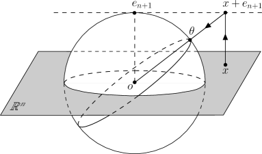
Figure 1: $\mu:\,x\rightarrow\theta$.

A simple geometric argument shows that $|x|=(1-\theta^{2}_{n+1})^{1/2}/|\theta_{n+1}|$ and the inequalities $|x|>a$ and $|\theta_{n+1}|<(1+a^{2})^{-1/2}$ are equivalent for every $a\geq 0$. Moreover, if $f$ is even, then (6.3) and (2.19) yield

$$\int\limits_{|x|>a}\!\!\frac{f(\mu(x))}{(1+|x|^{2})^{(n+1)/2}}\,dx\!=\!\frac{1}{2}\int\limits_{|\theta_{n+1}|<\alpha}\!\!\!f(\theta)\,d\theta,\qquad\alpha\!=\!(1\!+\!a^{2})^{-1/2},$$ (6.4)

provided that at least one of these integrals exists in the Lebesgue sense.

The map $\mu$ extends to the bijection $\tilde{\mu}$ from the set $\Pi_{n}$ of all unoriented hyperplanes in ${\mathbb{R}}^{n}$ onto the set

$$\tilde{S}^{n}_{+}=\{\omega=(\omega_{1},\ldots,\omega_{n+1})\in S^{n}:\,0\leq\omega_{n+1}<1\}.$$ (6.5)

cf. (6.2). Specifically, if $\tau=\{x\in{\mathbb{R}}^{n}:x\cdot\eta=t\}\in\Pi_{n}$, $\eta\in S^{n-1}\subset{\mathbb{R}}^{n}$, $t\geq 0$, and $\tilde{\tau}$ is the $n$-dimensional subspace containing the lifted plane $\tau+e_{n+1}$, then $\omega\in\tilde{S}^{n}_{+}$ is defined to be a normal vector to $\tilde{\tau}$. A simple geometric consideration shows that

$$\omega=-\eta\,{\hbox{\rm cos}}\,\alpha+e_{n+1}\sin\alpha,\qquad\tan\alpha=t.$$ (6.6)

The above notation is used in the following theorem.

Theorem 6.1.

Let $g(x)=(1+|x|^{2})^{-n/2}f(\mu(x))$, $x\in{\mathbb{R}}^{n}$, where $f$ is an even function on $S^{n}$. The Funk transform $F$ and the Radon transform $R$ are related by the formula

$$(Ff)(\omega)=\frac{2}{\sigma_{n-1}\,\sin d(\omega,e_{n+1})}\,(Rg)(\tilde{\mu}^{-1}\omega),\qquad\omega\in\tilde{S}^{n}_{+},$$ (6.7)

where $d(\omega,e_{n+1})$ is the geodesic distance between $\omega$ and $e_{n+1}$.

Proof.

Since the operators on both sides of this equality commute with rotations about the $x_{n+1}$ axis, it suffices to prove the theorem when $\omega$ is the $\tilde{\mu}$-image of the hyperplane $\tau=\{x\in{\mathbb{R}}^{n}:x\cdot e_{n}=t\}$, that is, $\omega=-e_{n}\,{\hbox{\rm cos}}\,\alpha+e_{n+1}\sin\alpha$, where $\tan\alpha=t$, $0\leq\alpha<\pi/2$.

Let $\tilde{\omega}=e_{n}\,\sin\alpha+e_{n+1}{\hbox{\rm cos}}\,\alpha$. We denote by $r_{\omega}$ a rotation in the $(x_{n},x_{n+1})$-plane that takes $e_{n+1}$ to $\tilde{\omega}$. Changing variables and using (2.19), we obtain

$$(Ff)(\omega) = \int\limits_{S^{n}\cap\omega^{\perp}}f(\sigma)\,d_{\omega}\sigma=\int\limits_{S^{n-1}}f(r_{\omega}\zeta)\,d_{*}\zeta$$

$$= \frac{2}{\sigma_{n-1}}\int\limits_{{\mathbb{R}}^{n-1}}f(r_{\omega}\,e_{y})\,\frac{dy}{|y+e_{n+1}|^{n}},\qquad e_{y}=\frac{y+e_{n+1}}{|y+e_{n+1}|}.$$

Note that

$$r_{\omega}\,e_{y} = \frac{y+r_{\omega}e_{n+1}}{\sqrt{1+|y|^{2}}}=\frac{y+e_{n}\,\sin\alpha+e_{n+1}{\hbox{\rm cos}}\,\alpha}{\sqrt{1+|y|^{2}}}$$

$$= \frac{z+e_{n}\tan\alpha+e_{n+1}}{|z+e_{n}\tan\alpha+e_{n+1}|},\qquad z=\frac{y}{{\hbox{\rm cos}}\,\alpha}.$$

Hence,

$$(Ff)(\omega) = \!\frac{2}{\sigma_{n-1}\,{\hbox{\rm cos}}\,\alpha}\int\limits_{{\mathbb{R}}^{n-1}}\!\!f\left(\frac{z\!+\!e_{n}\tan\alpha\!+\!e_{n+1}}{|z\!+\!e_{n}\tan\alpha\!+\!e_{n+1}|}\right)\,\frac{dz}{(t^{2}\!+\!|z|^{2}\!+\!1)^{n/2}}$$

$$= \frac{2}{\sigma_{n-1}\,{\hbox{\rm cos}}\,\alpha}\int\limits_{{\mathbb{R}}^{n-1}}f(\mu(z+te_{n}))\,\frac{dz}{(t^{2}+|z|^{2}+1)^{n/2}}$$

$$= \frac{2}{\sigma_{n-1}\,\sin d(\omega,e_{n+1})}\,(Rg)(e_{n},t).$$

This gives the result. ∎

Theorem 6.1 enables us to essentially extend the classes of function $f$ for which the Funk transform $Ff$ is finite a.e. on $S^{n}$ and is injective. For example, Theorem 2.5 and (6.7) imply the following statement.

Theorem 6.2.

Let $f$ be an even function on $S^{n}$. If

$$\int\limits_{|\theta_{n+1}|<\alpha}|f(\theta)|\,d\theta<\infty\quad\forall\,\alpha\in(0,1),$$ (6.8)

then $(Ff)(\omega)$ is finite for almost all $\omega\in S^{n}$. If $f$ is nonnegative, zonal, and (6.8) fails, then $(Ff)(\omega)\equiv\infty$.

Proof.

Following Theorems 2.5 and 6.1, we need to transform the integral

$$I=\int\limits_{|x|>a}\frac{|g(x)|}{|x|}\,dx=\int\limits_{|x|>a}\frac{|f(\mu(x))|}{(1+|x|^{2})^{n/2}|x|}\,dx.$$

By (6.4), it can be written as

$$I=\frac{1}{2}\int\limits_{|\theta_{n+1}|<\alpha}f_{1}(\theta)\,d\theta,\qquad f_{1}(\mu(x))=|f(\mu(x))|\,\frac{(1+|x|^{2})^{1/2}}{|x|}\,,$$

$\alpha=(1+a^{2})^{-1/2}$. Since

$$\int\limits_{|\theta_{n+1}|<\alpha}f_{1}(\theta)\,d\theta=\int\limits_{|\theta_{n+1}|<\alpha}\frac{|f(\theta)|\,d\theta}{(1-\theta^{2}_{n+1})^{1/2}}\leq c_{\alpha}\int\limits_{|\theta_{n+1}|<\alpha}|f(\theta)|\,d\theta,$$

the results follows.

∎

Combining Theorem 6.1, (6.6) and (6.4) with Theorem 4.14, we arrive at the support theorem for the Funk transform.

Theorem 6.3.

For $\alpha\in(0,1)$, let

$$\mathcal{O}_{\alpha}=\{\theta\in S^{n}:\,|\theta_{n+1}|<\alpha\},\qquad\tilde{\mathcal{O}}_{\alpha}=\{\omega\in S^{n}:\,|\omega_{n+1}|>\sqrt{1-\alpha^{2}}\}.$$

If $f=0$ a.e. in $\mathcal{O}_{\alpha}$, then $Ff=0$ a.e. in $\tilde{\mathcal{O}}_{\alpha}$. Conversely, if

$$\int\limits_{\mathcal{O}_{\alpha}}|f(\theta)|\,|\theta_{n+1}|^{-m-1}\,d\theta<\infty\quad\forall\,m\in{\mathbb{N}}$$

and $Ff=0$ a.e. in $\tilde{\mathcal{O}}_{\alpha}$, then $f=0$ a.e. in $\mathcal{O}_{\alpha}$.

In a similar way, Theorems 4.10 and 4.11 yield the corresponding result for the kernel of the operator $F$. We know that $\ker F=\{0\}$ if the action of $F$ is considered on even integrable functions. The situation changes if the functions under consideration allow non-integrable singularities at the poles $\pm e_{n+1}$, so that the Funk transform still exists in the a.e. sense.

If $f$ is even, it suffices to consider the points $\theta\in S^{n}$ which are represented in the spherical polar coordinates as

$$\theta=\eta\,\sin\psi+e_{n+1}\,{\hbox{\rm cos}}\,\psi,\qquad\eta\in S^{n-1},\qquad 0<\psi<\pi/2.$$

The corresponding Fourier-Laplace coefficients (in the $\eta$-variable) have the form

$$f_{m,\mu}(\psi)=\int\limits_{S^{n-1}}f(\eta\,\sin\psi+e_{n+1}\,{\hbox{\rm cos}}\,\psi)\,Y_{m,\mu}(\eta)\,d\eta.$$ (6.9)

We write $f\neq 0$ if the set $\{\theta\in S^{n}:f(\theta)\neq 0\}$ has positive measure.

Theorem 6.4.

Let $f$ be an even function on $S^{n}$ such that

$$I_{1}(f)=\int\limits_{|\theta_{n+1}|<\alpha}|f(\theta)|\,d\theta<\infty\quad\mbox{for all $\;\alpha\in(0,1)$}.$$ (6.10)

(i)   Suppose that $f_{m,\mu}(\psi)=0$ for almost all $\psi\in(0,\pi/2)$ if $m=0,1$, and

$$f_{m,\mu}(\psi)=\sin^{-n}\psi\sum_{\begin{subarray}{c}k=0\\ m-k\,even\end{subarray}}^{m-2}c_{k}\,\cot^{k}\psi,\qquad c_{k}={\hbox{\rm const}},$$ (6.11)

if $m\geq 2$. Then $(Ff)(\omega)=0$ a. e. on $S^{n}$.

(ii)   Conversely, let $(Ff)(\omega)=0$ a. e. on $S^{n}$. Suppose, in addition to (6.10), that

$$I_{2}(f)=\int\limits_{|\theta_{n+1}|>\alpha}|f(\theta)|\,(1-\theta^{2}_{n+1})^{\gamma}\,d\theta<\infty$$ (6.12)

for some $\gamma>-1/2$ and $\alpha\in(0,1)$. Then each Fourier-Laplace coefficient $f_{m,\mu}(\psi)$ is a finite linear combination of the functions $\sin^{-n}\psi\,\cot^{k}\psi$, $k=0,1,\ldots$, and the following statements hold.

(a) If $m=0,1$, then $f_{m,\mu}(\psi)\equiv 0$.

(b) If $m\geq 2$ and $f\neq 0$, then $f_{m,\mu}(\psi)\not\equiv 0$ for at least one pair $(m,\mu)$. For every such pair, $f_{m,\mu}(\psi)$ has the form (6.11).

Proof.

By Theorem 6.1, it suffices to reformulate our statement in terms of the function $g(x)=(1+|x|^{2})^{-n/2}f(\mu(x))$ and then apply Theorems 4.10 and 4.11. One can readily check that the assumptions of these theorems (with $f$ replaced by $g$) are equivalent to the corresponding assumptions in Theorem 6.4 and (6.11) mimics (4.29). ∎

Example 6.5.

Let $\{Y_{m,\mu}\}$ be a fixed real-valued orthonormal basis of spherical harmonics in $L^{2}(S^{n-1})$. Consider any function of the form

$$f(\theta)\!=\!\frac{Y_{2,\mu}(\theta^{\prime}/|\theta^{\prime}|)}{(1\!-\!\theta^{2}_{n+1})^{n/2}},\quad\theta^{\prime}\!=\!(\theta_{1},\ldots,\theta_{n}),\quad\mu\!=\!1,2,\ldots,\frac{(n\!+\!2)(n\!-\!1)}{2}.$$

This function is even and satisfies the assumptions of Theorem 6.4 for any $\gamma>n/2$. Moreover, if $\theta=\eta\,\sin\psi+e_{n+1}\,{\hbox{\rm cos}}\,\psi$, $\eta\in S^{n-1}$, $0<\psi<\pi/2$, then

$$f_{2,\mu}(\psi)=\sin^{-n}\psi\int\limits_{S^{n-1}}[Y_{m,\mu}(\eta)]^{2}\,d\eta=\sin^{-n}\psi.$$

Hence, by Theorem 6.4, $Ff=0$ a.e. on $S^{n}$. In fact, $(Ff)(\omega)=0$ for all $\omega$ away from the poles $\pm e_{n+1}$. To see that, it suffices to smoothen $f$ in arbitrarily small neighborhoods of the poles.

Remark 6.6.

As in the Euclidean case, where the origin $(0,\ldots,0)$ is fixed (cf. Remark 4.13), here we fix the north pole $(0,\ldots,0,1)$. If we choose another point as a pole, the statement of Theorem 6.4 will be modified accordingly.

7. The Spherical Slice Transform

Let $S^{n}$ be the unit sphere in ${\mathbb{R}}^{n+1}$, $n\geq 2$. We denote by $\Gamma(S^{n})$ the set of all $(n-1)$-dimensional geodesic spheres $\gamma\subset S^{n}$ passing through the north pole $e_{n+1}$. Every $\gamma$ is a cross-section of $S^{n}$ by the corresponding hyperplane. Below we consider an integral transform that assigns to a function $f$ on $S^{n}$ a function $\hbox{\frak S}f$ on $\Gamma(S^{n})$ by the formula

$$(\hbox{\frak S}f)(\gamma)=\int\limits_{\gamma}f(\eta)\,d_{\gamma}\eta,$$ (7.1)

where $d_{\gamma}\eta$ denotes the usual surface element on $\gamma$. The map $f\to\hbox{\frak S}f$ is called the spherical slice transform of $f$.

Every geodesic sphere $\gamma\in\Gamma(S^{n})$ can be indexed by its center $\xi=(\xi_{1},\ldots,\xi_{n+1})$ in the the closed hemisphere

$$\bar{S}^{n}_{+}=\{\xi=(\xi_{1},\ldots\xi_{n+1})\in S^{n}:\;0\leq\xi_{n+1}\leq 1\},$$

so that

$$\gamma\equiv\gamma(\xi)=\{\eta\in S^{n}:\eta\cdot\xi=e_{n+1}\cdot\xi\},\qquad\xi\in\bar{S}^{n}_{+}.$$

If $\xi_{n+1}=1$, then $\gamma(\xi)$ boils down to one point, the north pole. If $\xi_{n+1}=0$, then $\gamma(\xi)$ is a “great circle” through the poles $\pm e_{n+1}$.

The operator (7.1) has an intimate connection with the Cauchy problem for the Darboux equation on $S^{n}$:

$$\delta_{\xi}u\!-\!u_{\omega\omega}\!-\!(n\!-\!1)\cot\omega\,u_{\omega}\!=\!0,\qquad u(\xi,0)\!=\!f(\xi),\quad u_{\omega}(\xi,0)\!=\!0.$$ (7.2)

Here $\xi\in S^{n}$ is the space variable, $\omega\in(0,\pi)$ is the time variable, $\delta_{\xi}$ is the Beltrami-Laplace operator acting on $u(\xi,\omega)$ in the $\xi$-variable. If $(M_{\xi}f)(t)$ is the spherical mean

$$(M_{\xi}f)(t)=\frac{(1-t^{2})^{(1-n)/2}}{\sigma_{n-1}}\int\limits_{\xi\cdot\eta=t}f(\eta)\,d\eta,\qquad t\in(-1,1),$$ (7.3)

then the function $u(\xi,\omega)=(M_{\xi}f)({\hbox{\rm cos}}\,\omega)$ is the solution to the problem (7.2); see, e.g., [47, 48].

The corresponding inverse problem is formulated as follows:

Let $d(\xi,e_{n+1})$ be the geodesic distance between the point $\xi$ and the north pole $e_{n+1}$. Given the trace $u(\xi,d(\xi,e_{n+1}))$ of the solution $u(\xi,\omega)$ of (7.2) on the conical set

$$\{(\xi,\omega):\,\xi\in\bar{S}^{n}_{+},\;\omega=d(\xi,e_{n+1})\},$$

reconstruct the initial function $f$.

One can easily see that $u(\xi,d(\xi,e_{n+1}))$ is exactly our slice transform (7.1) with $\gamma=\gamma(\xi)$.

Using spherical coordinates, for $\xi\in\bar{S}^{n}_{+}$ we write

$$\xi=\theta\sin\psi+e_{n+1}\,{\hbox{\rm cos}}\,\psi,\qquad\theta\in S^{n-1}\subset{\mathbb{R}}^{n},\quad 0\leq\psi\leq\pi/2,$$

$$\gamma=\gamma(\xi)=\gamma(\theta,\psi),\qquad(\hbox{\frak S}f)(\gamma)=(\hbox{\frak S}f)(\xi)=(\hbox{\frak S}f)(\theta,\psi).$$

Then

$$\gamma(\xi)=\{\eta\in S^{n}:\eta\cdot\xi={\hbox{\rm cos}}\,\psi\}.$$

Consider the bijective mapping

$${\mathbb{R}}^{n}\ni x\xrightarrow{\;\nu\;}\eta\in S^{n}\setminus\{e_{n+1}\},\qquad\nu(x)=\frac{2x+(|x|^{2}-1)\,e_{n+1}}{|x|^{2}+1}.$$ (7.4)

The inverse mapping $\nu^{-1}:S^{n}\setminus\{e_{n+1}\}\rightarrow{\mathbb{R}}^{n}$ is the stereographic projection from the north pole $e_{n+1}$ onto ${\mathbb{R}}^{n}={\mathbb{R}}e_{1}\oplus\cdots\oplus{\mathbb{R}}e_{n}$. If

$$\eta=\omega\,\sin\varphi+e_{n+1}{\hbox{\rm cos}}\,\varphi,\qquad\omega\in S^{n-1},\qquad 0<\varphi\leq\pi,$$

then $x=\nu^{-1}(\eta)=s\omega$, $s=\cot(\varphi/2)$; see Figure 2.

Figure 2: $\eta=\omega\,\sin\varphi+e_{n+1}{\hbox{\rm cos}}\,\varphi,\quad|x|=\cot(\varphi/2)$.

We shall show that the spherical slice transform on $S^{n}$ can be expressed through the hyperplane Radon transform on ${\mathbb{R}}^{n}$ by making use of this projection.

The following statement is a counterpart of Lemma 2.4 and can be found in the literature in different forms; see, e.g., [43]. For the sake of completeness, we present it with a simple proof.

Lemma 7.1.

(i) If $f\in L^{1}(S^{n})$, then

$$\int\limits_{S^{n}}f(\eta)\,d\eta=2^{n}\int\limits_{{\mathbb{R}}^{n}}(f\circ\nu)(x)\,\frac{dx}{(|x|^{2}+1)^{n}}.$$ (7.5)

(ii) If $g\in L^{1}({\mathbb{R}}^{n})$, then

$$\int\limits_{{\mathbb{R}}^{n}}g(x)\,dx=\int\limits_{S^{n}}(g\circ\nu^{-1})(\eta)\,\frac{d\eta}{(1-\eta_{n+1})^{n}}.$$ (7.6)

Proof.

(i) Passing to spherical coordinates, we have

$$l.h.s. = \int\limits_{0}^{\pi}\sin^{n-1}\varphi\,d\varphi\int\limits_{S^{n-1}}\!\!f(\omega\,\sin\varphi+e_{n+1}\,{\hbox{\rm cos}}\,\varphi)\,d\omega$$

($$s=\cot(\varphi/2)$$)

$$= 2^{n}\int\limits_{0}^{\infty}\frac{s^{n-1}ds}{(s^{2}+1)^{n}}\int\limits_{S^{n-1}}\!\!\!f\left(\frac{2s\omega\!+\!(s^{2}\!-\!1)\,e_{n+1}}{s^{2}+1}\right)\,d\omega\!=\!r.h.s.$$

(ii) We set $g(x)=2^{n}(|x|^{2}+1)^{-n}(f\circ\nu)(x)$ in (7.5). Since

$$|x|^{2}+1=s^{2}+1=\cot^{2}(\varphi/2)+1=\frac{2}{1-{\hbox{\rm cos}}\varphi}=\frac{2}{1-\eta_{n+1}},$$ (7.7)

the result follows. ∎

Lemma 7.2.

The spherical slice transform on $S^{n}$ and the hyperplane Radon transform on ${\mathbb{R}}^{n}$ are linked by the formula

$$(\hbox{\frak S}f)(\theta,\psi)=(Rg)(\theta,t),\qquad t=\cot\psi,$$ (7.8)

$$g(x)=\left(\frac{2}{|x|^{2}+1}\right)^{n-1}(f\circ\nu)(x),$$ (7.9)

provided that either side of (7.8) is finite when $f$ is replaced by $|f|$.

Proof.

To prove the lemma, we combine the stereographic projection with translation and rotation. Since both S and $R$ commute with rotations about the $x_{n+1}$-axis, it suffices to assume $\theta=e_{n}=(0,\ldots,0,1,0)$. Let $\tau_{\gamma}$ be the hyperplane containing $\gamma=\gamma(e_{n},\psi)$, and let $o^{\prime}\in\tau_{\gamma}$ be the center of the sphere $\gamma$. A simple calculation shows that

$$o^{\prime}=e_{n}{\hbox{\rm cos}}\psi\sin\psi+e_{n+1}\,{\hbox{\rm cos}}^{2}\psi.$$ (7.10)

We translate $\tau_{\gamma}$ so that $o^{\prime}$ moves to the origin $o=(0,\ldots,0)$. Then we rotate the translated plane $\tau_{\gamma}-o^{\prime}$, making it coincident with the coordinate plane $e_{n}^{\perp}$ and keeping the subspace ${\mathbb{R}}^{n-1}={\mathbb{R}}e_{1}\oplus\ldots\oplus{\mathbb{R}}e_{n}$ fixed. Let $\tilde{\gamma}\subset e_{n}^{\perp}$ be the image of $\gamma$ under this transformation. We stretch $\tilde{\gamma}$ up to the unit sphere $S^{n-1}$ in $e_{n}^{\perp}$ and project $S^{n-1}$ stereographically onto ${\mathbb{R}}^{n-1}$; see Figure 3.

Figure 3: $\gamma=o^{\prime}+\rho\tilde{\gamma},\;r=\sin\psi$.

Thus, can write

$$\gamma=o^{\prime}+\rho\tilde{\gamma},\quad\rho=\left[\begin{array}[]{cc}I_{n-1}&0\\ 0&\rho_{\psi}\end{array}\right],\quad\rho_{\psi}=\left[\begin{array}[]{cc}\sin\psi&-{\hbox{\rm cos}}\psi\\ {\hbox{\rm cos}}\psi&\sin\psi\end{array}\right],$$ (7.11)

$$(\hbox{\frak S}f)(e_{n},\psi)\!=\!\int\limits_{\tilde{\gamma}}f(o^{\prime}\!+\!\rho\sigma)\,d_{\tilde{\gamma}}\sigma\!=\!r^{n-1}\int\limits_{S^{n-1}}f(o^{\prime}\!+\!\rho r\sigma)\,d\sigma,\quad r\!=\!\sin\psi.$$

By Lemma 7.1 (with $n$ replaced by $n-1$), we obtain

$$(\hbox{\frak S}f)(\theta,\psi)=(2r)^{n-1}\int\limits_{{\mathbb{R}}^{n-1}}f(o^{\prime}+\rho r\tilde{\nu}(y))\,\frac{dy}{(|y|^{2}+1)^{n-1}},$$

$$\tilde{\nu}(y)=\frac{2y+(|y|^{2}-1)\,e_{n+1}}{|y|^{2}+1}.$$

The expression under the sign of $f$ can be transformed using (7.10) and (7.11):

$$o^{\prime}\!+\!\rho r\tilde{\nu}(y)=\frac{A}{|y|^{2}+1},$$

$$A = (|y|^{2}+1)(e_{n}{\hbox{\rm cos}}\psi\sin\psi+e_{n+1}\,{\hbox{\rm cos}}^{2}\psi)$$

$$+ [2y+(|y|^{2}\!-\!1)(-e_{n}{\hbox{\rm cos}}\psi+e_{n+1}\sin\psi)]\,\sin\psi$$

$$= 2y\sin\psi+e_{n}\sin 2\psi+e_{n+1}(|y|^{2}+{\hbox{\rm cos}}2\psi).$$

Hence,

$$(\hbox{\frak S}f)(e_{n},\psi)=(2\sin\psi)^{n-1}$$

$$\times\int\limits_{{\mathbb{R}}^{n-1}}\!\!\!f\left(\frac{2y\sin\psi+e_{n}\sin 2\psi+e_{n+1}(|y|^{2}\!+\!{\hbox{\rm cos}}2\psi)}{|y|^{2}+1}\right)\,\frac{dy}{(|y|^{2}\!+\!1)^{n-1}}.$$

Changing variable $y=u\sin\psi$ and setting $t=\cot\psi$, this expression can be represented as

$$2^{n-1}\!\!\int\limits_{{\mathbb{R}}^{n-1}}\!\!\!f\left(\frac{2(u\!+\!te_{n})\!+\!(|u\!+\!te_{n}|^{2}\!-\!1)\,e_{n+1}}{|u+te_{n}|^{2}+1}\right)\,\frac{du}{(|u\!+\!te_{n}|^{2}\!+\!1)^{n-1}}.$$

The latter is the Radon transform $(Rg)(e_{n},t)$ with $g$ defined by (7.9). ∎

Lemma 7.2 enables us to investigate the slice transform S using properties of the hyperplane Radon transform $R$. For example, Theorem 2.5, combined with (7.7) and Lemma 7.1, gives the following result.

Theorem 7.3.

If

$$\int\limits_{\eta_{n+1}>1-\varepsilon}\frac{|f(\eta)|}{(1-\eta_{n+1})^{1/2}}\,d\eta<\infty\quad\forall\,0<\varepsilon\leq 2,$$ (7.12)

then $(\hbox{\frak S}f)(\xi)$ is finite for almost all $\xi\in S^{n}_{+}$. If $f$ is nonnegative, zonal, and (7.12) fails, then $(\hbox{\frak S}f)(\xi)\equiv\infty$.

The next statement, which mimics Theorem 5.3, is another consequence of (7.7) and Lemma 7.1.

Theorem 7.4.

If

$$(1-\eta_{n+1})^{n-1-n/p}f(\eta)\in L^{p}(S^{n}),\qquad 1\leq p<\frac{n}{n-1},$$ (7.13)

then $f$ can be uniquely reconstructed from $\hbox{\frak S}f$ by the formula

$$f(\eta)=(1-\eta_{n+1})^{1-n}(R^{-1}F\circ\nu)(\eta),$$ (7.14)

where $F(\theta,t)=(\hbox{\frak S}f)(\theta,\cot^{-1}t)$ and $R^{-1}$ is the inverse Radon transform.

A simple calculation shows that the injectivity condition (7.13) is stronger than the existence condition (7.12).

Corollary 7.5.

The operator S is injective on the class of functions $f$ for which $(1-\eta_{n+1})^{-1}f(\eta)\in L^{1}(S^{n})$. Moreover, it is injective on $L^{\infty}(S^{n})$.

Proof.

The first statement is contained in Theorem 7.4 (set $p=1$). The second one follows from the observation that every bounded function satisfies (7.13) with $p$ sufficiently close to $n/(n-1)$. ∎

If $f$ is zonal, then $\hbox{\frak S}f$ is zonal too and can be represented by the Erdélyi-Kober type fractional integral. To this end, we set

$$\eta=\omega\,\sin\varphi+e_{n+1}\,{\hbox{\rm cos}}\,\varphi,\qquad\omega\in S^{n-1},\qquad 0<\varphi\leq\pi.$$

Since $f$ is zonal, then $f(\eta)$ depends only on $\varphi$. We denote $f(\eta)=f_{0}(\cot\varphi/2)$. Similarly, if

$$\xi=\theta\sin\psi+e_{n+1}\,{\hbox{\rm cos}}\,\psi,\qquad\theta\in S^{n-1},\qquad 0\leq\psi\leq\pi/2,$$

then $(\hbox{\frak S}f)(\xi)$ depends only on $\psi$. We set $(\hbox{\frak S}f)(\xi)=F_{0}(\cot\psi)$.

Theorem 7.6.

If $f$ is a zonal function satisfying (7.12), then

$$F_{0}(t)=2^{n-1}\sigma_{n-2}\int\limits^{\infty}_{t}\frac{f_{0}(r)}{(1+r^{2})^{n-1}}\,(r^{2}-t^{2})^{(n-3)/2}\,r\,dr.$$ (7.15)

Proof.

Since $f$ is zonal, then $g$ in (7.8) is radial. We set $g(x)=\tilde{g}(|x|)$. By (2.24) and Lemma 7.2,

$$F_{0}(t)=\sigma_{n-2}\int\limits^{\infty}_{t}\!\tilde{g}(r)(r^{2}-t^{2})^{(n-3)/2}r\,dr.$$

It remains to express $\tilde{g}$ through $f_{0}$. We have

$$g(x)=\frac{2^{n-1}\,(f\circ\nu)(x)}{(1+|x|^{2})^{n-1}},\qquad|x|=|\nu(\eta)|=\cot\varphi/2;$$

cf. (7.9) and (7.7). Hence,

$$\tilde{g}(r)=\frac{2^{n-1}\,f_{0}(r)}{(1+r^{2})^{n-1}},$$

and we are done. ∎

Another application of the Radon transform theory is related to the spherical harmonic decomposition of $f(\eta)=f(\omega\sin\varphi+e_{n+1}\,{\hbox{\rm cos}}\,\varphi)$ in the $\omega$-variable. Let

$$f_{m,\mu}(\varphi)=\int\limits_{S^{n-1}}f(\omega\sin\varphi+e_{n+1}\,{\hbox{\rm cos}}\,\varphi)\,Y_{m,\mu}(\omega)\,d\omega.$$

Then Theorems 4.10 and 4.11 in conjunction with Lemma 7.2 imply the following description of the kernel of the operator S.

Theorem 7.7.

Let

$$I_{1}(f)=\int\limits_{\eta_{n+1}>1-\varepsilon}\frac{|f(\eta)|}{(1-\eta_{n+1})^{1/2}}\,d\eta<\infty\quad\forall\,\varepsilon\in(0,2].$$ (7.16)

(i)   Suppose that $f_{m,\mu}(\varphi)=0$ for almost all $\varphi\in(0,\pi)$ if $m=0,1$, and

$$f_{m,\mu}(\varphi)\!=\!(1\!-\!{\hbox{\rm cos}}\,\varphi)^{1-n}\sum_{\begin{subarray}{c}k=0\\ m-k\,even\end{subarray}}^{m-2}\!c_{k}\,\left(\tan\frac{\varphi}{2}\right)^{n+k},\quad c_{k}\!=\!{\hbox{\rm const}},$$ (7.17)

if $m\geq 2$. Then $(\hbox{\frak S}f)(\xi)=0$ a.e. on $S^{n}$.

(ii)   Conversely, let $(\hbox{\frak S}f)(\xi)=0$ a. e. on $S^{n}$. Suppose, in addition to (7.16), that

$$I_{2}(f)=\int\limits_{\eta_{n+1}<1-\varepsilon}|f(\eta)|\,(1+\eta_{n+1})^{\lambda}\,d\eta<\infty$$ (7.18)

for some $\lambda>-1/2$ and $0<\varepsilon\leq 2$. Then each Fourier-Laplace coefficient $f_{m,\mu}(\varphi)$ is a finite linear combination of the functions

$$(1-{\hbox{\rm cos}}\,\varphi)^{1-n}\,\left(\tan\frac{\varphi}{2}\right)^{n+k},\qquad k=0,1,\ldots,$$

and the following statements hold.

(a) If $m=0,1$, then $f_{m,\mu}(\varphi)\equiv 0$.

(b) If $m\geq 2$ and $f\neq 0$, that is, the set $\{\eta:f(\eta)\neq 0\}$ has positive measure, then $f_{m,\mu}(\varphi)\not\equiv 0$ for at least one pair $(m,\mu)$. For every such pair, $f_{m,\mu}(\varphi)$ has the form (7.17).

In a similar way, Theorem 4.14 implies the support theorem for the slice transform.

Theorem 7.8.

Given $a\in(0,1)$, consider the spherical caps

$$\Omega_{a}\!=\!\{\eta\in S^{n}:\,\eta_{n+1}>a\},\qquad\tilde{\Omega}_{a}\!=\!\{\xi\in S^{n}:\,\xi_{n+1}>\sqrt{(1\!+\!a)/2}\,\}.$$

If $f=0$ a.e. in $\Omega_{a}$, then $\hbox{\frak S}f=0$ a.e. in $\tilde{\Omega}_{a}$. Conversely, if

$$\int\limits_{\Omega_{a}}(1-\eta_{n+1})^{-1-m/2}\,|f(\eta)|\,d\eta<\infty\quad\forall\,m\in{\mathbb{N}}$$

and $\hbox{\frak S}f=0$ a.e. in $\tilde{\Omega}_{a}$, then $f=0$ a.e. in $\Omega_{a}$.

8. The Totally Geodesic Radon Transform on the Hyperbolic Space

We will be dealing with the hyperboloid model of the $n$-dimensional real hyperbolic space ${\mathbb{H}}^{n}$ which is described in [27]; see also [7]. Let ${\mathbb{E}}^{n,1}\sim{\mathbb{R}}^{n+1}$, $n\geq 2$, be the $(n+1)$-dimensional pseudo-Euclidean real vector space with the inner product

$$[{\bf x},{\bf y}]=-x_{1}y_{1}-\ldots-x_{n}y_{n}+x_{n+1}y_{n+1}.$$ (8.1)

The space ${\mathbb{H}}^{n}$ is realized as the upper sheet of the two-sheeted hyperboloid in ${\mathbb{E}}^{n,1}$, that is,

$${\mathbb{H}}^{n}=\{{\bf x}\in{\mathbb{E}}^{n,1}:\|{\bf x}\|^{2}=1,\ x_{n+1}>0\}.$$

The corresponding one-sheeted hyperboloid is defined by

$$\overset{*}{{\mathbb{H}}}{}^{n}=\{{\bf x}\in E^{n,1}:\|{\bf x}\|^{2}=-1\}.$$

Both ${\mathbb{H}}^{n}$ and $\overset{*}{{\mathbb{H}}}{}^{n}$ are orbits of the identity component $G=SO_{0}(n,1)$ of the special pseudo-orthogonal group $SO(n,1)$ of linear transformations preserving the bi-linear form $[{\bf x},{\bf y}]$ and having the determinant $1$.

Unlike the boldfaced ${\bf x},{\bf y}\in{\mathbb{E}}^{n,1}$, the usual letters $x,y$ will be used for points in ${\mathbb{H}}^{n}$. The geodesic distance between $x$ and $y$ is defined by $d(x,y)={\hbox{\rm cosh}}^{-1}[x,y]$. We fix the $G$-invariant measure $dx$ on ${\mathbb{H}}^{n}$ which is normalized so that

$$\int\limits_{{\mathbb{H}}^{n}}\!f(x)\,dx=\int\limits_{0}^{\infty}{\hbox{\rm sinh}}^{n-1}r\,dr\int\limits_{S^{n-1}}\!\!f(\theta\,{\hbox{\rm sinh}}r+e_{n+1}{\hbox{\rm cosh}}r)\,d\theta$$ (8.2)

for every $f\in L^{1}({\mathbb{H}}^{n})$. The totally geodesic Radon transform of a function $f$ on ${\mathbb{H}}^{n}$ is defined by the formula

$$(\hbox{\frak R}f)(\xi)=\int\limits_{\{x\in{\mathbb{H}}^{n}:\,[x,\xi]=0\}}f(x)\,d_{\xi}x,\qquad\xi\in\overset{*}{{\mathbb{H}}}{}^{n},$$ (8.3)

and represents an even function on $\overset{*}{{\mathbb{H}}}{}^{n}$. The corresponding dual transform of an even function $\varphi$ on $\overset{*}{{\mathbb{H}}}{}^{n}$ has the form

$$(\hbox{\frak R}^{\ast}\varphi)(x)=\int\limits_{\{\xi\in\overset{*}{{\mathbb{H}}}{}^{n}:\,[x,\xi]=0\}}\!\!\varphi(\xi)\,d_{x}\xi,\qquad x\in{\mathbb{H}}^{n}.$$ (8.4)

The measures $d_{\xi}x$ and $d_{x}\xi$ are $G$-images of the corresponding measures on the sets

$${\mathbb{H}}^{n-1}=\{y\in{\mathbb{H}}^{n}:\,y_{n}=0\},\qquad S^{n-1}=\{\eta\in\overset{*}{{\mathbb{H}}}{}^{n}:\,\eta_{n+1}=0\}.$$

Specifically, let $\omega_{x}$ and $\omega_{\xi}$ be hyperbolic rotations in $G$ satisfying

$$\omega_{x}:\,e_{n+1}\to x,\qquad\omega_{\xi}:\,e_{n}\to\xi.$$ (8.5)

If $f_{\xi}(y)=f(\omega_{\xi}y)$ and $\varphi_{x}(\eta)=\varphi(\omega_{x}\eta)$, then the precise meaning of the above integrals is the following:

$$(\hbox{\frak R}f)(\xi)=\int\limits_{{\mathbb{H}}^{n-1}}f_{\xi}(y)\,dy,\qquad(\hbox{\frak R}^{\ast}\varphi)(x)=\int\limits_{S^{n-1}}\varphi_{x}(\eta)\,d_{*}\eta.$$ (8.6)

Both R and $\hbox{\frak R}^{\ast}$ are $G$-invariant.

Let $S^{n-1}$ and $S^{n-2}$ be the unit spheres in the coordinate planes ${\mathbb{R}}^{n}={\mathbb{R}}e_{1}\oplus\ldots\oplus{\mathbb{R}}e_{n}$ and ${\mathbb{R}}^{n-1}={\mathbb{R}}e_{1}\oplus\ldots\oplus{\mathbb{R}}e_{n-1}$, respectively. The notation

$$a_{r}=\left[\begin{array}[]{ccc}I_{n-1}&0&0\\ 0&{\hbox{\rm cosh}}r&{\hbox{\rm sinh}}r\\ 0&{\hbox{\rm sinh}}r&{\hbox{\rm cosh}}r\end{array}\right]$$ (8.7)

is used for the corresponding hyperbolic rotation in the plane $(x_{n},x_{n+1})$. Given $x\in{\mathbb{H}}^{n}$ and $\xi\in\overset{*}{{\mathbb{H}}}{}^{n}$, we set

$$x\! = \!\theta\,{\hbox{\rm sinh}}r\!+\!e_{n+1}{\hbox{\rm cosh}}r\!=\!\omega_{\theta}a_{r}e_{n+1},\quad\,\theta\in S^{n-1},\;r\in{{\mathbb{R}}}_{+},$$ (8.8)

$$\xi\! = \!\sigma\,{\hbox{\rm cosh}}\rho\!+\!e_{n+1}{\hbox{\rm sinh}}\rho\!=\!\omega_{\sigma}a_{\rho}e_{n},\qquad\sigma\in S^{n-1},\;\rho\in{{\mathbb{R}}}.$$ (8.9)

Here $\omega_{\theta}$ and $\omega_{\sigma}\in SO(n)$ are arbitrary rotations satisfying $\omega_{\theta}e_{n}=\theta$, $\omega_{\sigma}e_{n}=\sigma$; $a_{\rho}$ has the same meaning as $a_{r}$ in (8.7).

Lemma 8.1.

Let $f_{\sigma}(x)=f(\omega_{\sigma}x)$, $\varphi_{\theta}(\xi)=\varphi(\omega_{\theta}\xi)$. Then

$$(\hbox{\frak R}f)(\xi)\!\! = \!\!\int\limits^{\infty}_{0}{\hbox{\rm sinh}}^{n-2}s\,ds$$

$$\times \!\!\int\limits_{S^{n-2}}\!\!f_{\sigma}(\omega\,{\hbox{\rm sinh}}s+(e_{n}\,{\hbox{\rm sinh}}\rho+e_{n+1}\,{\hbox{\rm cosh}}\rho)\,{\hbox{\rm cosh}}s)\,d\omega,$$

$$(\hbox{\frak R}^{*}\varphi)(x)\!\!\! = \!\!\!\int\limits_{S^{n-1}}\!\!\!\varphi_{\theta}(\eta^{\prime}+e_{n}\,\eta_{n}\,{\hbox{\rm cosh}}r+e_{n+1}\,\eta_{n}\,{\hbox{\rm sinh}}r)\,d_{*}\eta,$$ (8.11)

$\eta\!=\!(\eta^{\prime},\eta_{n})$, provided that the corresponding integrals exist in the Lebesgue sense.

Proof.

Consider the totally geodesic Radon transform (8.3) and set $x=\omega_{\sigma}a_{\rho}y$, where $\sigma$ and $a_{\rho}$ are the same as in (8.9). We have

$$(\hbox{\frak R}f)(\xi) = \int\limits_{{\mathbb{H}}^{n-1}}f_{\sigma}(a_{\rho}y)\,dy$$

$$= \int\limits^{\infty}_{0}{\hbox{\rm sinh}}^{n-2}s\ ds\int\limits_{S^{n-2}}f_{\sigma}(a_{\rho}(\omega\,{\hbox{\rm sinh}}s+e_{n+1}\,{\hbox{\rm cosh}}s)\,d\omega.$$

This gives (8.1). Further, setting $\xi=\omega_{\theta}a_{r}\eta$ in (8.4), we obtain

$$(\hbox{\frak R}^{*}\varphi)(x)\!=\!\int\limits_{S^{n-1}}\!\!\varphi_{\theta}(a_{r}\eta)\,d_{*}\eta\!=\!\int\limits_{S^{n-1}}\!\!\varphi_{\theta}(\eta^{\prime}\!+\!e_{n}\,\eta_{n}\,{\hbox{\rm cosh}}r\ \!+\!e_{n+1}\,\eta_{n}\,{\hbox{\rm sinh}}r)\,d_{*}\eta.$$

∎

The totally geodesic transform (8.3) and its dual (8.4) are intimately connected with the hyperplane Radon transform $R$ and its dual $R^{*}$. To establish this connection we fix the notation by setting

$$(Rg)(\sigma,t)\!=\!\int\limits_{\sigma^{\perp}}g(\sigma t\!+\!u)\,d_{\sigma}u,\qquad(R^{\ast}h)(y)\!=\!\int\limits_{S^{n-1}}h(\sigma,y\cdot\sigma)\,d_{*}\sigma.$$ (8.12)

Here $t\in{\mathbb{R}}$ and $\sigma^{\perp}$ is the subspace of ${\mathbb{R}}^{n}$ orthogonal to $\sigma\in S^{n-1}$. Let

$$x=\theta\,{\hbox{\rm sinh}}r\!+\!e_{n+1}{\hbox{\rm cosh}}r,\qquad\,\theta\in S^{n-1},\;r\in{{\mathbb{R}}}_{+},$$

$$\xi=\sigma\,{\hbox{\rm cosh}}\rho\!+\!e_{n+1}{\hbox{\rm sinh}}\rho,\qquad\sigma\in S^{n-1},\;\rho\in{{\mathbb{R}}}.$$

We also write $\;\tilde{x}=(x_{1},\ldots,x_{n}),\quad\tilde{\xi}=(\xi_{1},\ldots,\xi_{n})$,

$$x=(\tilde{x},x_{n+1})=(\theta\,{\hbox{\rm sinh}}r,{\hbox{\rm cosh}}r)\in{\mathbb{H}}^{n},$$

$$\xi=(\tilde{\xi},\xi_{n+1})=(\sigma\,{\hbox{\rm cosh}}\rho,{\hbox{\rm sinh}}\rho)\in\overset{*}{{\mathbb{H}}}{}^{n},$$

$$f(x)\equiv f(\theta\,{\hbox{\rm sinh}}r,{\hbox{\rm cosh}}r),\qquad\varphi(\xi)\equiv\varphi(\sigma{\hbox{\rm cosh}}\rho,{\hbox{\rm sinh}}\rho).$$

To every $x\!=\!(\tilde{x},x_{n+1})\in{\mathbb{H}}^{n}$ we associate its image $y$ in the tangent hyperplane to ${\mathbb{H}}^{n}$ at the point $(0,\ldots,0,1)\in{\mathbb{H}}^{n}$, so that $x$ and $y$ lie on the same line through the origin $(0,\ldots,0,0)$ of $E^{n,1}$. If this tangent hyperplane is identified with the Euclidean space ${\mathbb{R}}^{n}$, then the map $x\to y$ is a bijection between ${\mathbb{H}}^{n}$ and the unit ball $B_{n}=\{y\in{\mathbb{R}}^{n}:\ |y|<1\}$, so that

$$y=\frac{\tilde{x}}{x_{n+1}},\qquad x\!=\!(\tilde{x},x_{n+1})=\left(\frac{y}{\sqrt{1-|y|^{2}}},\frac{1}{\sqrt{1-|y|^{2}}}\right).$$ (8.13)

Under this map, every totally geodesic submanifold of ${\mathbb{H}}^{n}$ is associated with a chord in $B_{n}$ of the same dimension. The corresponding functions on ${\mathbb{R}}^{n}$ and $Z_{n}=S^{n-1}\times{\mathbb{R}}$ are defined by

$$g(y)=(1-|y|^{2})^{-n/2}_{+}f\left(\frac{y}{\sqrt{1-|y|^{2}}},\frac{1}{\sqrt{1-|y|^{2}}}\right),\qquad y\in{\mathbb{R}}^{n},$$ (8.14)

$$h(\sigma,t)=(1-t^{2})^{-n/2}_{+}\varphi\left(\frac{\sigma}{\sqrt{1-t^{2}}},\frac{t}{\sqrt{1\!-\!t^{2}}}\right),\quad\sigma\in S^{n-1},\;t\in{\mathbb{R}},$$ (8.15)

so that

$$f(x)=\frac{g(\tilde{x}/x_{n+1})}{x^{n}_{n+1}}=\frac{g(\theta\,{\hbox{\rm tanh}}r)}{{\hbox{\rm cosh}}^{n}r}\,,$$ (8.16)

$$\varphi(\xi)=(1+\xi^{2}_{n+1})^{-n/2}\;\!h\left(\frac{\tilde{\xi}}{\sqrt{1+\xi^{2}_{n+1}}},\frac{\xi_{n+1}}{\sqrt{1+\xi^{2}_{n+1}}}\right)=\frac{h(\sigma,{\hbox{\rm tanh}}\rho)}{{\hbox{\rm cosh}}^{n}\rho}\,.$$ (8.17)

Lemma 8.2.

For every $\delta\geq 0$,

$$\int\limits_{d(x,e_{n+1})>\delta}f(x)\,\frac{dx}{x_{n+1}}=\int\limits_{{\rm tanh}\delta<|y|<1}g(y)\,dy$$ (8.18)

provided that either integral exists in the Lebesgue sense.

Proof.

We have

$$r.h.s.\!=\!\int\limits_{{\rm tanh}\delta}^{1}s^{n-1}\,ds\int\limits_{S^{n-1}}g(\theta s)\,d\theta\!=\!\int\limits_{\delta}^{\infty}\frac{{\hbox{\rm tanh}}^{n-1}r}{{\hbox{\rm cosh}}^{2}r}\,dr\int\limits_{S^{n-1}}\!g(\theta\,{\hbox{\rm tanh}}r)\,d\theta.$$

By (8.2) and (8.16), this expression coincides with the left-hand side. ∎

Lemma 8.3.

The following equalities hold provided that the integral in either side exists in the Lebesgue sense:

$$(\hbox{\frak R}f)(\xi)=\frac{1}{{\hbox{\rm cosh}}\rho}\,(Rg)(\sigma,{\hbox{\rm tanh}}\rho),$$ (8.19)

$$(\hbox{\frak R}^{*}\varphi)(x)=\frac{1}{{\hbox{\rm cosh}}r}\,(R^{\ast}h)(\theta\,{\hbox{\rm tanh}}r).$$ (8.20)

Proof.

Let $\omega_{\theta}$, $\omega_{\sigma}\!\in\!SO(n)$ be arbitrary rotations satisfying $\omega_{\theta}e_{n}\!=\!\theta$, $\omega_{\sigma}e_{n}\!=\!\sigma$. We write $g_{\sigma}(y)=g(\omega_{\sigma}y)$. By (8.1) and (8.16),

$$(\hbox{\frak R}f)(\xi) = \int\limits^{\infty}_{0}{\hbox{\rm sinh}}^{n-2}s\ ds\int\limits_{S^{n-2}}g_{\sigma}\left(\omega\,\frac{{\hbox{\rm tanh}}s}{{\hbox{\rm cosh}}\rho}+e_{n}\,{\hbox{\rm tanh}}\rho\right)\,\frac{d\omega}{({\hbox{\rm cosh}}s\,{\hbox{\rm cosh}}\rho)^{n}}$$

(set $$t={\hbox{\rm tanh}}s/{\hbox{\rm cosh}}\rho$$)

$$= \int\limits^{\infty}_{0}\frac{t^{n-2}dt}{{\hbox{\rm cosh}}\rho}\int\limits_{S^{n-2}}g_{\sigma}(\omega\,t\!+\!e_{n}\,{\hbox{\rm tanh}}\rho)\,d\omega$$

$$= \frac{1}{{\hbox{\rm cosh}}\rho}\int\limits_{{\mathbb{R}}^{n-1}}g_{\sigma}(v\!+\!e_{n}\,{\hbox{\rm tanh}}\rho)\,dv.$$

The last expression coincides with (8.19). Let us prove (8.20). Denoting $h_{\theta}(\sigma,t)=h(\omega_{\theta}\sigma,t)$ and using (8.11) and (8.17), we have

$$(\hbox{\frak R}^{*}\varphi)(x)\!=\!\frac{1}{\sigma_{n-1}}\int\limits^{1}_{-1}(1\!-\!\eta^{2}_{n})^{(n-3)/2}d\eta_{n}$$

$$\times\int\limits_{S^{n-2}}\varphi_{\theta}\left(\omega\,\sqrt{1\!-\!\eta^{2}_{n}}\!+\!e_{n}\eta_{n}{\hbox{\rm cosh}}r+e_{n+1}\eta_{n}\,{\hbox{\rm sinh}}r\right)\,d\omega$$

or

$$(\hbox{\frak R}^{*}\varphi)(x)\!=\!\frac{1}{\sigma_{n-1}}\int\limits^{1}_{-1}\frac{(1\!-\!\eta^{2}_{n})^{(n-3)/2}\,d\eta_{n}}{(1\!+\!\eta^{2}_{n}\,{\hbox{\rm sinh}}^{2}r)^{n/2}}$$

$$\times\int\limits_{S^{n-2}}\!h_{\theta}\left(\frac{\omega\,\sqrt{1\!-\!\eta^{2}_{n}}\!+\!e_{n}\eta_{n}{\hbox{\rm cosh}}r}{\sqrt{1+\zeta^{2}_{n}\,{\hbox{\rm sinh}}^{2}r}},\frac{\eta_{n}{\hbox{\rm sinh}}r}{\sqrt{1\!+\!\eta^{2}_{n}\,{\hbox{\rm sinh}}^{2}r}}\right)d\omega.$$

Setting $\eta_{n}=\zeta_{n}/\sqrt{{\hbox{\rm cosh}}^{2}r-\zeta^{2}_{n}\,{\hbox{\rm sinh}}^{2}r}$, we continue

$$(\hbox{\frak R}^{*}\varphi)(x)\!=\!\frac{1}{\sigma_{n-1}\,{\hbox{\rm cosh}}r}\int\limits^{1}_{-1}(1\!-\!\zeta^{2}_{n})^{(n-3)/2}d\zeta_{n}$$

$$\times\int\limits_{S^{n-2}}h_{\theta}(\omega\,\sqrt{1\!-\!\zeta^{2}_{n}}\!+\!e_{n}\zeta_{n},\,\zeta_{n}{\hbox{\rm tanh}}r)\,d\omega$$

$$=\frac{1}{{\hbox{\rm cosh}}r}\int\limits_{S^{n-1}}h_{\theta}(\zeta,(\zeta\cdot e_{n})\,{\hbox{\rm tanh}}r)\,d_{*}\zeta=\frac{1}{{\hbox{\rm cosh}}r}\,(R^{\ast}h)(\theta\,{\hbox{\rm tanh}}r).$$

∎

Lemmas 8.2 and 8.3 combined with Theorem 2.5 yield the following existence result for the totally geodesic transform R.

Theorem 8.4.

If

$$\int\limits_{d(x,e_{n+1})>a}|f(x)|\,\frac{dx}{x_{n+1}}<\infty$$ (8.21)

for all $a>0$, then $(\hbox{\frak R}f)(\xi)$ is finite for almost all $\xi\in\overset{*}{{\mathbb{H}}}{}^{n}$. If $f$ is nonnegative, zonal, and (8.21) fails for some $a>0$, then $(\hbox{\frak S}f)(\xi)\equiv\infty$.

In a similar way, the support theorem the Radon transform $R$ (see Theorem 4.14) implies the following statement.

Theorem 8.5.

Let $a>0$ and let $\tau_{\xi}$ denote the totally geodesic submanifold in ${\mathbb{H}}^{n}$ indexed by $\xi\!\in\!\overset{*}{{\mathbb{H}}}{}^{n}$. If $f(x)=0$ for almost all $x\!\in\!{\mathbb{H}}^{n}$ satisfying $d(x,e_{n+1})\!>\!a$, then $(\hbox{\frak R}f)(\xi)\!=\!0$ for almost all $\xi$ satisfying $d(\tau_{\xi},e_{n+1})>a$. Conversely, if $f$ satisfies (8.21) and $(\hbox{\frak R}f)(\xi)\!=\!0$ for almost all $\xi$ with $d(\tau_{\xi},e_{n+1})>a$, then $f(x)=0$ for almost all $x\in{\mathbb{H}}^{n}$ satisfying $d(x,e_{n+1})>a$.

We observe an amazing fact that, unlike the Euclidean case in Theorem 4.14, the above theorem does not require a rapid decay of $f$ at infinity. This fact was discovered by Kurusa [35]. The reason is that the function $g$ in (8.19) is supported in the unit ball and therefore, the condition (4.30) holds automatically. Note also that the condition $d(\tau_{\xi},e_{n+1})>a$ is equivalent to $|\xi_{n+1}|>{\hbox{\rm sinh}}\,a$, and $d(x,e_{n+1})\!>\!a$ is equivalent to $x_{n+1}>{\hbox{\rm cosh}}\,a$.

Theorems 4.10 and 4.11 give the corresponding result for the kernel of the operator R. We write $x\in{\mathbb{H}}^{n}$ in the hyperbolic polar coordinates as $x=\theta\,{\hbox{\rm sinh}}r+e_{n+1}\,{\hbox{\rm cosh}}r$, $\theta\in S^{n-1}$, $r>0$, and compute the Fourier-Laplace coefficients

$$f_{m,\mu}(r)=\int\limits_{S^{n-1}}f(\theta\,{\hbox{\rm sinh}}r+e_{n+1}{\hbox{\rm cosh}}r)\,Y_{m,\mu}(\theta)\,d\theta.$$ (8.22)

Theorem 8.6.

Let

$$I_{1}(f)=\int\limits_{x_{n+1}>1+\delta}|f(x)|\,\frac{dx}{x_{n+1}}<\infty\quad\forall\,\delta>0.$$ (8.23)

(i)   Suppose that $f_{m,\mu}(r)=0$ for almost all $r>0$ if $m=0,1$, and

$$f_{m,\mu}(r)={\hbox{\rm sinh}}^{-n}r\sum_{\begin{subarray}{c}k=0\\ m-k\,even\end{subarray}}^{m-2}c_{k}\,\coth^{k}\psi,\qquad c_{k}={\hbox{\rm const}},$$ (8.24)

if $m\geq 2$. Then $(\hbox{\frak R}f)(\xi)=0$ a. e. on $\overset{*}{{\mathbb{H}}}{}^{n}$.

(ii)  Conversely, let $(\hbox{\frak R}f)(\xi)=0$ a. e. on $\overset{*}{{\mathbb{H}}}{}^{n}$. Suppose additionally that

$$I_{2}(f)=\int\limits_{x_{n+1}<1+\delta}|f(x)|\,(x_{n+1}-1)^{\lambda}\,dx<\infty$$ (8.25)

for some $\delta>0$ and $\lambda>-1/2$. Then each Fourier-Laplace coefficient $f_{m,\mu}(r)$ is a finite linear combination of the functions ${\hbox{\rm sinh}}^{-n}r\,\coth^{k}\psi$, $k=0,1,\ldots$, and the following statements hold.

(a) If $m=0,1$, then $f_{m,\mu}(r)\equiv 0$.

(b) If $m\geq 2$ and $f\neq 0$, that is, the set $\{x:f(x)\neq 0\}$ has positive measure, then $f_{m,\mu}(r)\not\equiv 0$ for at least one pair $(m,\mu)$. For every such pair, $f_{m,\mu}(r)$ has the form (8.24).

Analogues of Theorems 8.5 and 8.6 for the dual transform $\hbox{\frak R}^{*}$ can be similarly derived from Theorems 4.15 and 4.5, respectively, using the connection (8.20). The corresponding results are left to the interested reader.

We conclude the paper by the following

Open Problem. Keeping in mind that the Gegenbauer-Chebyshev integrals (and the corresponding Radon transforms) have unilateral structure, we wonder if the following assumptions caused by the method of the proof can be omitted:

$\bullet$ $\;\varphi\in S^{\prime}(Z_{n})$ in Theorem 4.6,

$\bullet$ $\;f\in S^{\prime}({\mathbb{R}}^{n})$ in Theorem 5.4(ii),

$\bullet$ $\;I_{2}(f)<\infty$ in Theorems 4.11, 6.4(ii), 7.7(ii), 8.6(ii).

Acknowledgements. I am grateful to Jan Boman, Sigurdur Helgason, Ricardo Estrada, Gestur Ólafsson, and Yuri Luchko for useful comments and discussion. My special thanks for the figures in this paper go to Emily Ribando-Gros who was supported by the NSF VIGRE program.

References

[1] A. Abouelaz and R. Daher, Sur la transformation de Radon de la sphère ,
Bull. Soc. Math. France 121 (1993), 353–-382.
[2] M. Agranovsky, P. Kuchment, and L. Kunyansky, On reconstruction formulas and algorithms for the thermoacoustic tomography.
In Photoacoustic imaging and spectroscopy, edited by L. Wang, CRC Press, 2009, pp. 89–102.
[3] D. H. Armitage, A non-constant continuous function on the plane whose integral on every line is zero, Amer. Math. Monthly 101 (1994), no. 9, 892–894.
[4] D. H. Armitage and M. Goldstein, Nonuniqueness for the Radon transform, Proc. Amer. Math. Soc. 117 (1993), no. 1, 175–178.
[5] C. A. Berenstein and E. Casadio Tarabusi, Range of the -dimensional Radon transform in real hyperbolic spaces, Forum Math. 5 (1993), 603–616.
[6] C. A. Berenstein, E. Casadio Tarabusi, and A. Kurusa, Radon transform on spaces of constant curvature, Proc. Amer. Math. Soc. 125 (1997), 455–461.
[7] C. A. Berenstein and B. Rubin,
Radon transform of -functions on the Lobachevsky space and
hyperbolic wavelet transforms, Forum Math.
11 (1999), 567–590.
[8] C. A. M. van Berkel, Integral transformations and spaces of type , Dissertation, Technische Universiteit Eindhoven, Eindhoven, 1992. Technische Universiteit Eindhoven, Eindhoven, 1992. vi+143 pp.
[9] C. A. M. van Berkel and S. J. L. van Eijndhoven, Fractional calculus, Gegenbauer transformations, and integral equations, J. Math. Anal. Appl. 194, no. 1 (1995), 126–146.
[10] J. Boman, Helgason’s support theorem for Radon transforms—a new proof and a generalization, Mathematical methods in tomography (Oberwolfach, 1990), 1–5, Lecture Notes in Math. 1497, Springer, Berlin, 1991.
[11] by same author, Holmgren’s uniqueness theorem and support theorems for real analytic Radon transforms, Geometric analysis (Philadelphia, PA, 1991), 23–30, Contemp. Math. 140, Amer. Math. Soc., Providence, RI, 1992.
[12] by same author, An example of nonuniqueness for a generalized Radon transform, J. Anal. Math. 61 (1993), 395–401.
[13] by same author, Support theorems for the Radon transform and Cramér-Wold theorems, J. of Theor. Probability 22, (2009), 683–710.
[14] J. Boman and E. T. Quinto, Support theorems for real-analytic Radon transforms, Duke Math. J. 55 (1987), 943–948.
[15] by same author, Support theorems for Radon transforms on real analytic line complexes in three-space, Trans. Amer. Math. Soc. 335 (1993), no. 2, 877–890.
[16] Y. W. Chen, On the solutions of the wave equation in a quadrant of , Bull. of the Amer. Math. Soc. 70 (1964), no. 1, 172–177.
[17] by same author, On the solutions of the wave equation in the exterior of the characteristic cones, J. Math. Mech. 16 (1967), 655–673.
[18] J. Cnops, The Gegenbauer transformation and singular value decompositions for the Radon transformation, Rend. Istit. Mat. Univ. Trieste (1-2) 27 (1995), 175–193 (1996).
[19] A. M. Cormack, Representation of a function by its line integrals, with some radiological applications, J. Appl. Phys. 34 (1963), 2722–2727.
[20] A. M. Cormack and E. T. Quinto, A Radon transform on spheres through the origin in and applications to the Darboux equation, Trans. Amer. Math. Soc. 260 (1980), no. 2, 575–581.
[21] R. Courant and D. Hilbert. Methods of mathematical physics. Vol. II. Partial differential equations, Interscience Publishers, New York-London-Sydney, 1962.
[22] S. R. Deans, The Radon transform and some of its applications, Dover Publ. Inc., Mineola, New York, 2007.
[23] A. Erdélyi (Editor), Higher transcendental functions, Vol. I
and II, McGraw-Hill, New York, 1953.
[24] P. G. Funk, Über Flächen mit lauter geschlossenen geodätischen Linien, Thesis, Georg-August-Universit t Göttingen, 1911.
[25] by same author, Über Flächen mit lauter geschlossenen geodätschen Linen, Math. Ann., 74 (1913), 278–300.
[26]
I.M. Gel’fand, S.G. Gindikin, and M.I. Graev, Selected topics
in integral geometry, Translations of Mathematical Monographs, AMS,
Providence, Rhode Island, 2003.
[27] I.M. Gel’fand, M.I. Graev, and N.Ja. Vilenkin,
Generalized
functions, Vol 5, Integral geometry and representation theory,
Academic Press, 1966.
[28] F. B. Gonzalez, and E. T. Quinto, Support theorems for Radon transforms on higher rank symmetric spaces,
Proc. Amer. Math. Soc. (4) 122 (1994), 1045–1052.
[29] S. Helgason, The Radon transform on symmetric
spaces, An address delivered before the Summer AMS Meeting on August 30, 1963, in Boulder, Colorado, by invitation of the Committee to select hour speakers for Annual and Summer Meetings.
[30] by same author, A duality in integral geometry; some generalizations of the Radon transform, Bull. Amer. Math. Soc. 70 (1964) 435–446.
[31] by same author, The Radon transform on Euclidean spaces, compact two-point
homogeneous spaces and Grassmann manifolds, Acta Math. 113 (1965),
153–180.
[32] by same author, Geometric analysis on symmetric
spaces, Second Edition, Amer. Math. Soc., Providence, RI, 2008.
[33] by same author, Integral geometry and Radon transform,
Springer, New York-Dordrecht-Heidelberg-London, 2011.
[34] P. Kuchment, The Radon transform and medical imaging, CBMS-NSF Regional Conference Series in Applied Mathematics, 85. Society for Industrial and Applied Mathematics (SIAM), Philadelphia, PA, 2014.
[35] Á. Kurusa, Support theorems for totally
geodesic Radon transforms
on constant curvature spaces, Proc. Amer. Math. Soc.
122 (1994), 429–435.
[36] P.D. Lax and R.S. Phillips, Spectral theory for the wave equation, unpublished notes, 1962.
[37] P.I. Lizorkin, Generalized Liouville differentiation and
functional spaces . Imbedding theorems, Matem. Sb.
60(120) (1963), 325–353 (In Russian).
[38] by same author, Generalized Liouville differentiation and the
method of multipliers in the theory of imbeddings of classes of
differentiable functions, Proc. Steklov Inst. Math. 105 (1969), 105–202.
[39] by same author, Description of the spaces in terms of difference singular integrals, Mat. Sb. 81 (123) (1970), 79–91 (In Russian).
[40] by same author, Operators connected with fractional differentiation and classes of
differentiable functions, Proc. Steklov Inst. Math. 117 (1972), 251–286.
[41] D. Ludwig, The Radon transform on Euclidean space, Comm. Pure
Appl. Math. 19 (1966), 49–81.
[42] O. I. Marichev, Method of evaluation of integrals of special functions,
Nauka i Technika, Minsk, 1978 (In Russian);
Engl. translation: Handbook of integral transforms of higher transcendental functions: Theory and Algorithmic Tables,
Ellis Horwood Ltd., N. York etc.; Halsted Press, 1983.
[43] S. G. Mikhlin, Multidimensional Singular Integrals and Integral Equations. Pergamon Press, Oxford, 1965.
[44] C. Müller, Spherical harmonics, Springer, Berlin, 1966.
[45] F. Natterer, The mathematics of computerized tomography, SIAM, Philadelphia, 2001.
[46] T. Ohsawa and T. Takiguchi, Abel-type integral transforms and the exterior problem for the Radon transform, Inverse Probl. Sci. Eng. 17 (2009), no. 4, 461–471.
[47] M. N. Olevsky, Quelques théorems de la moyenne dans les espaces à
courbure constante, C.R. (Dokl.) Acad Sci URSS 45 (1944), 95–98.
[48] by same author, On the equation is a linear operator)
and the solution of the Cauchy problem for the generalized equation of
Euler-Darboux,
Dokl. AN SSSR 93 (1953), 975–978 (Russian).
[49] V. Palamodov. Reconstructive Integral Geometry. Monographs in Mathematics, 98. Birkhäuser Verlag, Basel, 2004.
[50] R.M. Perry,
On reconstructing a function on the exterior of a disk from its Radon transform,
J. Math. Anal. Appl. 59 (1977), no. 2, 324–341.
[51] A. P. Prudnikov, Y. A. Brychkov, and O. I. Marichev, Integrals and series: special functions. Gordon and Breach Sci. Publ., New York-London, 1986.
[52] E.T. Quinto, Null spaces and ranges for the classical and spherical Radon transforms, J. Math. Anal. Appl. 90 (1982) 408–420.
[53] by same author, Singular value decompositions and inversion methods
for the exterior Radon transform and a spherical transform,
Journal of Math, Anal. and Appl. 95 (1983), 437–448.
[54] by same author, A note on flat Radon transforms. Geometric analysis (Philadelphia, PA, 1991), 115–121, Contemp. Math., 140, Amer. Math. Soc., Providence, RI, 1992.
[55] by same author, Real analytic Radon transforms on rank one symmetric spaces, Proc. Amer. Math. Soc. 117 (1993), 179–186.
[56] by same author, Helgason’s support theorem and spherical Radon transforms, Radon transforms, geometry, and wavelets, 249–264, Contemp. Math. 464, Amer. Math. Soc., Providence, RI, 2008.
[57] H. Rhee, A representation of the solutions of the Darboux equation in odd-dimensional spaces, Trans. Amer. Math. Soc. 150 (1970), 491–498.
[58] by same author, Expression for a function in terms of its spherical means, Bull. Amer. Math. Soc. 76 (1970) 626–628.
[59] B. Rubin, Inversion formulas for the spherical
Radon transform and the generalized cosine transform, Adv. in Appl.
Math. 29 (2002), 471-497.
[60] by same author, Reconstruction of functions from their integrals over
-dimensional planes, Israel J. of Math. 141 (2004), 93–117.
[61] by same author, On the Funk-Radon-Helgason inversion method in integral geometry, Cont. Math. 599 (2013), 175–198.
[62] S.G. Samko, Hypersingular integrals and their applications,
Taylor & Francis, 2002.
[63] S.G. Samko, A.A. Kilbas, and O.I.
Marichev, Fractional integrals
and derivatives. Theory and applications, Gordon and Breach Sc.
Publ., New York, 1993.
[64] R. T. Seeley, Spherical harmonics, No. 11 of the H. Ellsworth Slaught Memorial Papers, Amer. Math. Monthly (4) 73 Part 2: Papers in Analysis (1966), 115–121.
[65] V.I. Semyanistyi, On some integral transformations in
Euclidean space, Dokl. Akad. Nauk SSSR 134
(1960), 536–539 (In Russian).
[66] D.C. Solmon, Asymptotic formulas for the dual Radon transform and applications,
Math. Z. 195 (1987), no. 3, 321–343.
[67] E.M. Stein and G. Weiss, Introduction to Fourier analysis on Euclidean spaces,
Princeton Univ. Press, Princeton, NJ, 1971.
[68] R.S. Strichartz, Radon inversion—variations on a theme, Amer. Math. Monthly 89 (1982), 377–384.
[69] T. Takiguchi, Remarks on modification of Helgason’s support theorem, J. Inverse Ill-Posed Probl. 8 (2000), 573–579.
[70] by same author, Remarks on modification of Helgason’s support theorem. II, Proc. Japan Acad. Ser. A Math. Sci. 77 (2001), no. 6, 87–91.
[71] T. Takiguchi and A. Kaneko, Radon transform of hyperfunctions and support theorem, Hokkaido Math. J. 24 (1995), no. 1, 63–103.
[72] J. J. O. O. Wiegerinck, A support theorem for Radon transforms on , Nederl. Akad. Wetensch. Indag. Math. 47 (1985), 87–93.
[73] L. Zalcman, Uniqueness and nonuniqueness for the Radon transform, Bull. London Math. Soc. 14 (1982), no. 3, 241–245.