The dynamics of general relativistic isotropic stellar cluster models – Do relativistic extensions of the Plummer model exist?

Abstract

We show that the general relativistic theory of the dynamics of isotropic stellar clusters can be developed essentially along the same lines as the Newtonian theory. We prove that the distribution function can be derived from any isotropic momentum moment and that every higher-order moment of the distribution can be written as an integral over a zeroth-order moment.

We propose a mathematically simple expression for the distribution function of a family of isotropic general relativistic cluster models and investigate their dynamical properties. In the Newtonian limit, these models obtain a distribution function of the form $F(E)\propto(E-E_{0})^{\alpha}$, with $E$ binding energy and $E_{0}$ a constant that determines the model’s outer radius. The slope $\alpha$ sets the steepness of the distribution function and the corresponding radial density and pressure profiles. We show that the field equations only yield solutions with finite mass for $\alpha\leq 3.5$. Moreover, in the limit $\alpha\rightarrow 3.5$, only Newtonian models exist. In other words: within the context of this family of models, no general relativistic version of the Plummer model exists. The most strongly bound model within the family is characterized by $\alpha=2.75$ and a central redshift $z_{c}\approx 0.55$.

1 Introduction

The so-called Plummer model was introduced by Plummer (1911) as a description of the stellar density distribution in Galactic globular clusters (Plummer, 1911). Subsequently, Eddington (1916) showed that this spherically symmetric density profile could be derived from a phase-space distribution of the form

$$F(\epsilon)\propto(-\epsilon)^{7/2},$$ (1)

with $\epsilon=\psi+v^{2}/2$ the Newtonian specific energy of a star and $\psi$ the Newtonian gravitational potential of the stellar cluster (Dejonghe, 1987). This distribution function self-consistently generates a mass distribution with a gravitational potential

$$\psi(r)=-\frac{GM}{a}\frac{1}{\sqrt{1+\left(\frac{r}{a}\right)^{2}}}$$ (2)

and density profile

$$\rho(r)=\frac{3}{4\pi}\left(1+\left(\frac{r}{a}\right)^{2}\right)^{-\frac{5}{2}}\frac{M}{a^{3}}=\frac{3}{4\pi}\left(-\frac{a}{GM}\psi\right)^{5}\frac{M}{a^{3}}.$$ (3)

Here, $M$ is the total mass of the cluster and $a$ a scale length.

Certain general relativistic (GR) extensions of the Plummer model can already be found in the literature and we give an overview here. For instance, in the case of a spherically symmetric cluster, the density, the potential (or some generalization thereof), and the distribution function are all functions of one argument, so it makes sense to construct the metric around a single, unknown function of the radius, usually denoted simply by $f(r)$. An example, inspired by the Schwarzschild metric is

$$ds^{2}=\left(\frac{1-f}{1+f}\right)^{2}c^{2}dt^{2}-(1+f)^{4}(dr^{2}+r^{2}d\Omega^{2}).$$ (4)

In the Newtonian limit, $f(r)$ reduces to $-\psi/(2c^{2})$.

One approach is to choose $f(r)$ such that it produces a meaningful cluster model in the Newtonian limit, for instance by equating it to the gravitational potential of the Newtonian cluster. Nguyen & Lingam (2013) show how this technique can be used to recover GR extensions of the hypervirial models of which the Plummer model is a special case. Solving the time-time-component of the field equations yields a density that together with $f$, by construction, correctly reduces to the corresponding Newtonian potential-density pair. However, as these authors note, the pressure does not reduce to the expected Newtonian limit. This is because the underlying distribution function does not reduce to the proper Newtonian limit.

Another possibility is to equate the radial and tangential field equations, thus enforcing isotropy, and to solve the resulting equation for the metric. This solution can then be plugged in the time-time-component of the field equations to yield the density profile. Buchdahl (1964) has used this procedure to produce a cluster model with an equation of state analogous to that of the Plummer model, i.e. a polytrope with index $n=5$. Fackerell (1971), using a metric of the form

$$ds^{2}=e^{\nu(r)}c^{2}dt^{2}-e^{\lambda(r)}dr^{2}-r^{2}d\Omega^{2},$$ (5)

subsequently derived a rather unwieldy analytical expression for the distribution function of this model and showed that, unless the central value of the potential satisfies $\exp(\nu(0))>0.413$, it can show a “temperature inversion” in the sense that it is not a monotonically decreasing function of energy. Alternatively, one can impose the polytropic equation of state on the field equations, which yields a generalization of the Lane-Emden equation, and thus solve for the unknown function in the metric (Tooper, 1964; Kaufmann, 1967).

Both techniques avoid an explit calculation of the distribution function. Using a generalization of Eddington’s integral equation, it can, however, be determined from the density profile (Fackerell, 1968; Pogorelov & Kandrup, 1996). Unfortunately, this distribution function is not guaranteed to be positive everywhere in phase space, although necessary conditions for positivity have been derived (Suffern, 1977).

Since employing the Eddington integral equation can lead to rather cumbersome expressions for the distribution function and, moreover, the latter’s positivity is not guaranteed from the outset, we here advocate another approach. We first write down a mathematically simple distribution function that is everywhere positive and that reduces to a well-defined Newtonian limit. From this distribution function, the density and pressure profiles can be calculated. By construction, all moments of the distribution function will reduce to the proper Newtonian limit. Solving the field equations finally yields the metric. While such generalizations of Newtonian cluster models may not have the same equation of state as in the Newtonian limit, they have the benefit of having a mathematically simple, strictly non-negative distribution function with a properly defined, meaningful Newtonian limit. Our goal is to produce general relativistic cluster models with isotropic, polytropic distribution functions, to study their dynamical properties, and to investigate their Newtonian limits. In particular, we wish to study how the Newtonian polytropes, of which the well-known Plummer model is a special case, fit in this more general scheme of models.

In section 2, we develop the dynamical theory of general relativistic stellar cluster models and calculate the properties of models with isotropic, polytropic distribution functions. In section 3, we present our method for solving the field equations for such models. We end with a discussion of the models in section 4 and conclude in section 5.

2 Isotropic dynamical models for general relativistic stellar clusters

2.1 The internal dynamics of isotropic clusters

In general relativistic dynamics, the distribution function (DF) $F(x^{\mu},p^{i})d^{3}xd^{3}p$ counts the number of occupied world lines that intersect a 6-dimensional submanifold of the 8-dimensional phase space. This 6-dimensional submanifold consists of a 3-dimensional spatial hypersurface and its future mass hyperboloid. In the absence of particle creation/annihilation or collisions, the Lie derivative of the DF is zero, or

$$\left[p^{\mu}\frac{\partial}{\partial x^{\mu}}-\Gamma^{\mu}_{\alpha\beta}p^{\alpha}p^{\beta}\frac{\partial}{\partial p^{\mu}}\right]F(x,\vec{p})=0.$$ (6)

Let $\hat{p}^{\mu}$ be the components of the momentum 4-vector in a local orthonormal frame at rest, such that $\hat{p}_{0}^{2}-\sum_{i}\hat{p}_{i}^{2}=(mc)^{2}$, with $m$ the rest mass of a single star. In such a local orthonormal frame, tensor quantities of the form

$$T_{\mu\nu\ldots\kappa}(x)=\int\frac{\hat{p}_{\mu}\hat{p}_{\nu}\ldots\hat{p}_{\kappa}}{\hat{p}_{0}}F(x,\vec{p})d\hat{p}_{1}d\hat{p}_{2}d\hat{p}_{3}$$ (7)

can be defined. If the Lie derivative of the DF disappears, then all these quantities have zero covariant divergence. The most well-known such tensor quantities are those with one index (the stream density vector) and two indices (the energy-momentum tensor).

In an isotropic cluster, the DF depends only on $p_{0}$, the 0-component of the momentum 4-vector, which is a constant in a time-independent gravitating system (see below). Obviously, what matters in the above definition of the momentum moments of the DF is the number of instances of each momentum component. We therefore re-write these momentum moments as

$$\mu_{k,2m,2n,2l}(x)=\int{\hat{p}_{0}}^{k}\hat{p}_{1}^{2m}\hat{p}_{2}^{2n}\hat{p}_{3}^{2l}F(p_{0})\frac{d\hat{p}_{1}d\hat{p}_{2}d\hat{p}_{3}}{\hat{p}_{0}}.$$ (8)

Using the parameterization

$$\hat{p}_{0} =\sqrt{(mc)^{2}+p^{2}}$$

$$\hat{p}_{1} =p\cos\vartheta$$

$$\hat{p}_{2} =p\sin\vartheta\cos\varphi$$

$$\hat{p}_{3} =p\sin\vartheta\sin\varphi$$ (9)

this reduces to

$$\mu_{k,2m,2n,2l}(x) =\frac{1}{2\pi}\frac{\Gamma\left(m+\frac{1}{2}\right)\Gamma\left(n+\frac{1}{2}\right)\Gamma\left(l+\frac{1}{2}\right)}{\Gamma\left(m+n+l+\frac{3}{2}\right)}\times$$

$$\hskip 20.00003pt4\pi\int F(p_{0})\hat{p}_{0}^{k-1}p^{2(m+n+l)+2}dp.$$ (10)

Let $E$ be the energy of a star as measured by an obsever at rest at infinity, where the geometry of spacetime is essentially flat. The energy measured by a local observer at rest, denoted by $E_{\sf local}$, is linked to $E$ via

$$E=\sqrt{g_{00}}E_{\sf local}=e^{\phi/2}E_{\sf local}=cp_{0}.$$ (11)

The 0-momentum in the local orthonormal frame, $\hat{p}_{0}$, is related to the energy at infinity as

$$c\hat{p}_{0}=\frac{cp_{0}}{\sqrt{g_{00}}}=\frac{E}{\sqrt{g_{00}}}.$$ (12)

Therefore,

$$E^{2}-m^{2}c^{4}g_{00}=g_{00}p^{2}c^{2}$$ (13)

and

$$pdp=\frac{EdE}{c^{2}g_{00}}.$$ (14)

Then

$$\mu_{k,2m,2n,2l}(x) =\frac{1}{2\pi}\frac{\Gamma\left(m+\frac{1}{2}\right)\Gamma\left(n+\frac{1}{2}\right)\Gamma\left(l+\frac{1}{2}\right)}{\Gamma\left(m+n+l+\frac{3}{2}\right)}\times$$

$$\hskip 20.00003pt\mu_{k,2(m+n+l)}(x)$$ (15)

which defines the set of isotropic $k$-moments

$$\mu_{k,2q} =4\pi\int F(p_{0})\hat{p}_{0}^{k}\left(\hat{p}_{0}^{2}-m^{2}c^{2}\right)^{q+\frac{1}{2}}d\hat{p}_{0}$$

$$=\frac{(mc)^{2q+k+2}}{2^{q+\frac{3}{2}}E_{0}^{2q+k+2}}\tilde{\mu}_{k,2q}(E_{0}^{2})$$ (16)

with

$$\tilde{\mu}_{k,2q}(E_{0}^{2}) =$$

$$2^{q+\frac{5}{2}}\pi\int_{E_{0}^{2}}F(E^{2})\left(E^{2}\right)^{\frac{k-1}{2}}(E^{2}-E_{0}^{2})^{q+\frac{1}{2}}dE^{2}$$ (17)

and $E_{0}^{2}=(mc^{2})^{2}g_{00}$. Deriving this equation $q$ times with respect to $E_{0}^{2}$ leads to

$$\tilde{\mu}_{k,0}(E_{0}^{2})=\frac{(-1)^{q}}{(2q+1)!!}D^{q}_{E_{0}^{2}}\tilde{\mu}_{k,2q}(E_{0}^{2}).$$ (18)

Here,

$$(2q+1)!!=(2q+1)(2q-1)\ldots 1$$ (19)

indicates the double factorial. This equation is formally identical to equation (1.3.7) in Dejonghe (1986). We can therefore simply invoke equation (1.3.8) from that same work to invert the above expression and to write all higher order $k$-moments of the DF in terms of the zeroth-order $k$-moment:

$$\tilde{\mu}_{k,2q}(E_{0}^{2})=\frac{(2q+1)!!}{(q-1)!!}\int_{E_{0}^{2}}(E^{2}-E_{0}^{2})^{q-1}\tilde{\mu}_{k,0}(E^{2})dE^{2}.$$ (20)

With the aid of equation (1.3.12) from Dejonghe (1986), (17) can be inverted as

$$E^{k-1}F(E)$$

$$=\frac{1}{2^{q+\frac{5}{2}}\pi^{\frac{3}{2}}\Gamma\left(q+\frac{3}{2}\right)}D^{q+2}_{E^{2}}\int_{E^{2}}\frac{\tilde{\mu}_{k,2q}({E}_{0}^{2})}{\sqrt{{E}_{0}^{2}-E^{2}}}d{E}_{0}^{2}$$

$$=\frac{(mc)^{-2q-k-2}}{2\pi^{\frac{3}{2}}\Gamma\left(q+\frac{3}{2}\right)}D^{q+2}_{E^{2}}\int_{E^{2}}\frac{E_{0}^{2q+k+2}\mu_{k,2q}({E}_{0}^{2})}{\sqrt{{E}_{0}^{2}-E^{2}}}d{E}_{0}^{2}.$$ (21)

In particular, for $(q=0,k=2)$ and for $(q=1,k=0)$ the above inversion relation reduces to the two important special cases

$$EF(E) =\frac{1}{\pi^{2}m^{4}c^{3}}D^{2}_{E^{2}}\int_{E^{2}}\frac{E_{0}^{4}\rho(E_{0}^{2})}{\sqrt{E_{0}^{2}-E^{2}}}dE_{0}^{2}$$

$$\frac{1}{E}F(E) =\frac{2}{\pi^{2}m^{4}c^{5}}D^{3}_{E^{2}}\int_{E^{2}}\frac{E_{0}^{4}P(E_{0}^{2})}{\sqrt{E_{0}^{2}-E^{2}}}dE_{0}^{2}$$ (22)

with $\rho$ the mass density and $P$ the pressure. These are none other than the inversion relations derived by Fackerell (1968) and Pogorelov & Kandrup (1996). Here, we made use of the fact that

$$\mu_{2,0} =\frac{4\pi}{g_{00}^{2}c^{4}}\int F(E)E^{2}\sqrt{E^{2}-E_{0}^{2}}dE=\rho c$$

$$\mu_{0,2} =\frac{4\pi}{g_{00}^{2}c^{4}}\int F(E)\left(E^{2}-E_{0}^{2}\right)^{\frac{3}{2}}dE=\frac{3P}{c}$$ (23)

(Zel’dovich & Podurets, 1965; Occhionero & San Martini, 1974). Hence, we have shown that these two relations linking the density and pressure to the isotropic DF are simply specific cases of a more general link between the DF and any of its moments $\mu_{k,2q}$.

2.2 A generalized polytropic distribution function

For a static, spherically symmetric gravitational system, the metric can always be brought in the form

$$ds^{2}=e^{\phi(r)}c^{2}dt^{2}-\left(1-\frac{2GM(r)}{c^{2}r}\right)^{-1}dr^{2}-r^{2}d\Omega^{2},$$ (24)

with $M(r)$ the total gravitating mass interior to the areal radius $r$ and $\phi$ a potential function that, in the Newtonian limit, reduces to $2\psi/c^{2}$. We propose a distribution function of the form

$$F(E)=f_{0}\left(\frac{mc^{2}}{E}\right)^{2\beta}\left(\frac{m^{2}c^{4}e^{\Phi}-E^{2}}{m^{2}c^{2}}\right)^{\alpha},$$ (25)

with $\alpha$ and $\beta$ positive real numbers, $f_{0}$ a constant forefactor, and $\Phi=\phi(R)$, the value of the potential at the outer edge of the cluster at radius $r=R$.

For the isotropic distribution function given above, the energy density is given by

$$\rho c^{2} =\frac{4\pi}{c^{3}}e^{-2\phi}\int_{mc^{2}e^{\phi/2}}^{mc^{2}e^{\Phi/2}}F(E)E^{2}\sqrt{E^{2}-m^{2}c^{4}e^{\phi}}dE$$

$$=\pi^{3/2}\frac{\Gamma(\alpha+1)}{\Gamma\left(\alpha+\frac{5}{2}\right)}f_{0}m^{4}c^{3+2\alpha}e^{-2\phi}\left(e^{\Phi}-e^{\phi}\right)^{\alpha+\frac{3}{2}}\times$$

$$e^{\left(\frac{1}{2}-\beta\right)\Phi}{{}_{2}F_{1}}\left(\beta-\frac{1}{2},\alpha+1;\alpha+\frac{5}{2};\frac{e^{\Phi}-e^{\phi}}{e^{\Phi}}\right)$$ (26)

(Zel’dovich & Podurets, 1965; Occhionero & San Martini, 1974). Here, $\Gamma(x)$ is Euler’s gamma-function and ${{}_{2}F_{1}}(a,b;c;z)$ is the Gaussian hypergeometric function

$${{}_{2}F_{1}}(a,b;c;z) =\frac{\Gamma(c)}{\Gamma(b)\Gamma(c-b)}\int_{0}^{1}t^{b-1}(1-t)^{c-b-1}\frac{dt}{(1-zt)^{a}}$$

$$=\sum_{n\geq 0}\frac{(a)_{n}(b)_{n}}{(c)_{n}}\frac{z^{n}}{n!}$$ (27)

with $(q)_{n}$ the Pocchammer symbol, defined as $(q)_{n}=\Gamma(q+n)/\Gamma(q)$. We can choose a scale-length $a$ and denote the scaled radius by $x=r/a$. With the choice of a mass scale $M$, we can introduce the dimensionless parameter

$${\cal A}=\frac{c^{2}a}{2GM}.$$ (28)

If the mass scale $M$ is taken to coincide the model’s total mass, then $\cal A$ is simply the ratio of the scale-length $a$ to the model’s Schwarzschild radius. We can then take

$$f_{0}=\frac{3}{4\pi^{\frac{5}{2}}c^{3+2\alpha}}\frac{\Gamma\left(\alpha+\frac{5}{2}\right)}{\Gamma(\alpha+1)}\frac{M{\cal A}^{\alpha+\frac{3}{2}}}{m^{4}a^{3}}.$$ (29)

With this choice for the forefactor $f_{0}$, we find the following expression for the density

$$\rho(\phi) =\frac{3}{4\pi}{\cal A}^{\alpha+\frac{3}{2}}e^{-2\phi}\left(e^{\Phi}-e^{\phi}\right)^{\alpha+\frac{3}{2}}\times$$

$$e^{\left(\frac{1}{2}-\beta\right)\Phi}{{}_{2}F_{1}}\left(\beta-\frac{1}{2},\alpha+1;\alpha+\frac{5}{2};\frac{e^{\Phi}-e^{\phi}}{e^{\Phi}}\right)\frac{M}{a^{3}}.$$ (30)

Clearly, the choice $\beta=0.5$ yields the “simplest” mass density profile since in that case the hypergeometric function is identically one and

$$\rho(\phi)=\frac{3}{4\pi}{\cal A}^{\alpha+\frac{3}{2}}e^{-2\phi}\left(e^{\Phi}-e^{\phi}\right)^{\alpha+\frac{3}{2}}\frac{M}{a^{3}}.$$ (31)

The expression for the pressure follows from

$$P =\frac{4\pi}{3c^{3}}e^{-2\phi}\int_{mc^{2}e^{\phi/2}}^{mc^{2}e^{\Phi/2}}F(E)\left(E^{2}-(mc^{2})^{2}e^{\phi}\right)^{\frac{3}{2}}dE$$

$$=\frac{3}{4\pi}\frac{{\cal A}^{\alpha+\frac{3}{2}}}{(2\alpha+5)}e^{-\left(\beta+\frac{1}{2}\right)\Phi}e^{-2\phi}\left(e^{\Phi}-e^{\phi}\right)^{\alpha+\frac{5}{2}}$$

$$\hskip 30.00005pt\times{{}_{2}F_{1}}\left(\beta+\frac{1}{2},\alpha+1;\alpha+\frac{7}{2};\frac{e^{\Phi}-e^{\phi}}{e^{\Phi}}\right)\frac{Mc^{2}}{a^{3}}.$$ (32)

The proper mass density is given by

$$nm =\frac{4\pi m}{c^{3}}e^{-3\phi/2}\int_{mc^{2}e^{\phi/2}}^{mc^{2}e^{\Phi/2}}F(E)E\sqrt{E^{2}-m^{2}c^{4}e^{\phi}}dE$$

$$=\frac{3}{4\pi}{\cal A}^{\alpha+\frac{3}{2}}e^{-\beta\Phi}e^{-3\phi/2}\left(e^{\Phi}-e^{\phi}\right)^{\alpha+\frac{3}{2}}$$

$$\hskip 30.00005pt\times{{}_{2}F_{1}}\left(\beta,\alpha+1;\alpha+\frac{5}{2};\frac{e^{\Phi}-e^{\phi}}{e^{\Phi}}\right)\frac{M}{a^{3}},$$ (33)

with $n$ the stellar proper number density. The proper mass of the cluster is then

$$M_{p}(r)=4\pi\int_{0}^{r}\frac{n(r)mr^{2}dr}{\sqrt{1-\frac{2GM}{c^{2}r}}}.$$ (34)

The difference between the total proper mass $M_{p}(R)$ and the total gravitating mass $M(r)$ can be interpreted as the gravitational binding energy of the cluster. We will henceforth use the fractional binding energy

$$f=\frac{M_{p}(R)-M(R)}{M_{p}(R)}$$ (35)

as a measure for the stability of a cluster since analytical and numerical work has shown that radial instability sets in in clusters around the first maximum of $f$ (Fackerell, 1969; Shapiro & Teukolsky, 1985).

From $p_{\mu}p^{\mu}=(mc)^{2}$, $J=r^{2}p^{3}=mru^{\phi}$, and $p^{0}c=Ee^{-\phi}$, it follows that for a circular orbit in the $\theta=\pi/2$ plane the angular momentum is given by

$$J=\frac{r}{c}E\sqrt{e^{-\phi}-\left(\frac{mc^{2}}{E}\right)^{2}}.$$ (36)

For a given radius $r$, the energy of the circular orbit with that radius can be found by setting $dJ/dr=0$. This leads to

$$\frac{mc^{2}}{E}=\sqrt{\left(1-\frac{r}{2}\frac{d\phi}{dr}\right)e^{-\phi}}.$$ (37)

Plugging this into the expression for the angular momentum yields

$$\frac{u^{\phi}}{c}=\frac{E}{mc^{2}}\sqrt{\frac{r}{2}\frac{d\phi}{dr}e^{-\phi}}.$$ (38)

From the viewpoint of a distant observer, the velocity of a star on a circular orbit with radius $r$ is given by

$$v_{\sf circ}(r)=\frac{d\tau_{P}}{dt}u^{\phi}=\frac{mc^{2}}{E}e^{\phi}u^{\phi}=c\sqrt{\frac{r}{2}\frac{d\phi}{dr}e^{\phi}}$$ (39)

since the derivative of the star’s proper time $\tau_{P}$ with respect to coordinate time is

$$\frac{d\tau_{P}}{dt}=\frac{mc}{p^{0}}=\frac{mc^{2}}{E}e^{\phi}.$$ (40)

The radiation of a light source at rest at radius $r$, is observed at infinity to have undergone a gravitational redshift

$$z(r)=e^{-\phi(r)/2}-1.$$ (41)

This “redshift-from-rest” is a measure for how “relativistic” a given cluster model is. Where it was first thought that no stable models with a central redshift-from-rest $z(0)\gtrsim 0.5$ can exist (Zel’dovich & Podurets, 1965; Ipser, 1969; Occhionero & San Martini, 1974), more recent work has shown that arbitrarily large values for the central “redshift-from-rest” are possible in stable models. The first hint that large redshifts are possible came from numerical integrations of the relativistic Boltzmann equation (Rasio, Shapiro, Teukolsky, 1989) that was later on backed up by detailed analytical calculations (Merafina & Ruffini, 1995). It was subsequently shown in Bisnovatyi-Kogan et al. (1998); Bisnovatyi-Kogan & Merafina (2006) that arbitrarily large central redshifts are possible in stable models with a distribution function of the form $F(E)\propto\exp(-E/T)$, with $T$ the uniform kinetic temperature as observed from infinity, only if $T/mc^{2}\lesssim 0.06$. “Hotter” models are stable only for redshifts below $\approx 0.5$.

2.3 The Newtonian limit

In the Newtonian limit, we can employ the approximation

$$\frac{d\tau_{P}}{dt} =\frac{mc^{2}}{cp^{0}}=\frac{mc^{2}}{E}e^{\phi}$$

$$=\frac{1}{c}\frac{ds}{dt}\approx\sqrt{e^{\phi}-\left(\frac{v}{c}\right)^{2}},$$ (42)

or, in other words,

$$E \approx\frac{mc^{2}e^{\phi}}{\sqrt{e^{\phi}-\left(\frac{v}{c}\right)^{2}}}\approx mc^{2}\left(1+\frac{1}{2}\phi+\frac{1}{2}\frac{v^{2}}{c^{2}}\right)$$

$$\approx mc^{2}+m\left(\psi+\frac{1}{2}v^{2}\right)=mc^{2}+m\epsilon.$$ (43)

Here, $\epsilon$ is the Newtonian energy per unit mass. Moreover, $\hat{p}_{0}c\approx mc^{2}+\frac{1}{2}mv^{2}$.

These results can be used to calculate the Newtonian approximation for the isotropic momentum moments of the DF, given by expression (16):

$$\mu_{k,2q} \approx 4\pi(mc)^{k-1}\int F(E)p^{2q+2}dp$$

$$\approx(mc)^{k-1}\mu^{N}_{2q}(\psi).$$ (44)

Except for the inconsequential forefactor $(mc)^{k-1}$, this is the correct expression for the Newtonian isotropic momentum moment $\mu^{N}_{2q}(\psi)$.

Taking together $E\approx E_{0}\approx mc^{2}$, $D_{E^{2}}\approx\frac{1}{2m^{2}c^{2}}D_{\epsilon}$, $dE_{0}^{2}\approx 2m^{2}c^{2}d\psi$, and (44), the inversion formula for the DF can be written in the form

$$F(\epsilon)\approx\frac{1}{2^{q+2}\pi^{\frac{3}{2}}\Gamma\left(q+\frac{3}{2}\right)m^{2q+3}}D_{\epsilon}^{q+2}\int\frac{\mu^{N}_{2q}(\psi)}{\sqrt{2(\psi-\epsilon)}}d\psi,$$ (45)

the correct Newtonian expression for the DF in terms of a Newtonian momentum moment. For $q=0$, one obtains the important special case

$$F(\epsilon)\approx\frac{1}{2\pi^{2}m^{3}}D_{\epsilon}^{2}\int\frac{\rho(\psi)}{\sqrt{2(\psi-\epsilon)}}d\psi,$$ (46)

with $\rho$ the mass density.

In the Newtonian limit, the distribution function (25) becomes $F(E)\approx f_{0}\left[2(\Psi-\epsilon)\right]^{\alpha}$, with $\Psi=\psi(R)$, the value of the Newtonian gravitational potential at the outer edge of the cluster. For an infinitely extended system with $\alpha=7/2$ and $\Psi=\psi(\infty)=0$ this is $f_{\text{Plum}}(E)=f_{0}(-2\epsilon)^{7/2}$, the distribution function of the Newtonian Plummer model. The Newtonian limit of the distribution function does not depend on the parameter $\beta$: it only serves to change the slope of the DF for the most strongly relativistic models. In the Newtonian limit, the density reduces to

$$\rho(\psi)\approx\frac{3}{4\pi}\left(-\frac{a}{GM}(\Psi-\psi)\right)^{\alpha+\frac{3}{2}}\frac{M}{a^{3}}.$$ (47)

For a Plummer model, with $\alpha=7/2$, we retrieve the relation

$$\rho_{\text{Plum}}\approx\frac{3}{4\pi}\left(-\frac{a}{GM}\psi\right)^{5}\frac{M}{a^{3}}.$$ (48)

The proper density $nm$ reduces to the same expression as the gravitating mass density $\rho$, as it should. The Newtonian expression for the pressure is found to be

$$P\approx\frac{3}{2\pi(2\alpha+5)}\left(-\frac{a}{GM}(\Psi-\psi)\right)^{\alpha+\frac{5}{2}}\frac{GM^{2}}{a^{4}}.$$ (49)

For a Plummer model, we find

$$P_{\text{Plum}}\approx\frac{1}{8\pi}\left(-\frac{a}{GM}\psi\right)^{6}\frac{GM^{2}}{a^{4}}\propto\rho_{\text{Plum}}^{\frac{6}{5}}.$$ (50)

Clearly, these Newtonian models have equations of state of the form

$$P=K\rho^{\frac{2\alpha+5}{2\alpha+3}}=K\rho^{1+\frac{1}{n}}$$ (51)

for some constant $K$. They are polytropes with polytropic index

$$n=\alpha+\frac{3}{2}\geq 0.$$ (52)

The general relativistic cluster models, due to the presence of the hypergeometric functions in the expressions for the density and pressure, are not polytropes and have more complicated equations of state. Newtonian polytropes have finite mass for $n\in[0,5]$ and finite radius for $n\in[0,5[$. The Plummer model, with $n=5$ is the first polytropic model with infinite radius but still with finite mass. It is generally assumed that the condition $df/dE<0$ is a prerequisite for the radial stability of a cluster (Ipser, 1969; Fackerell, 1971). We therefore limit ourselves to models with $\alpha\geq 0$, and hence $n\geq\frac{3}{2}$, for which this condition is definitely fulfilled.

As is well known, the structure of a polytrope with index $n$ and equation of state $P=K\rho^{1+\frac{1}{n}}$ for some constant forefactor $K$ is given by the Lane-Emden equation

$$\frac{1}{\xi^{2}}\frac{d}{d\xi}\left(\xi^{2}\frac{d\theta}{d\xi}\right)=-\theta^{n}.$$ (53)

Here, $\xi$ is a dimensionless radius related to the radius $r$ via

$$\xi=\sqrt{\frac{2\pi c^{2}a^{3}}{(n+1){\cal A}M}\frac{\rho_{c}^{2}}{P_{c}}}\frac{r}{a},$$ (54)

with $\rho_{c}$ and $P_{c}$ the central density and pressure, respectively. This equation must be integrated numerically for the function $\theta(r)$ out to its first zero, which then defines the outer radius $R$ of the cluster. Then the density is given by $\rho(r)=\rho_{c}\theta^{n}(r)$, and the gravitational potential by $\psi(r)=-(n+1)K\rho_{c}^{\frac{1}{n}}\theta(r)+\psi(R)$. The circular velocity profile, $v_{\sf circ}(r)$, then follows from the relation

$$v_{\sf circ}(r)=\sqrt{r\frac{d\psi}{dr}}.$$ (55)

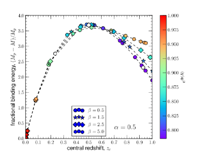
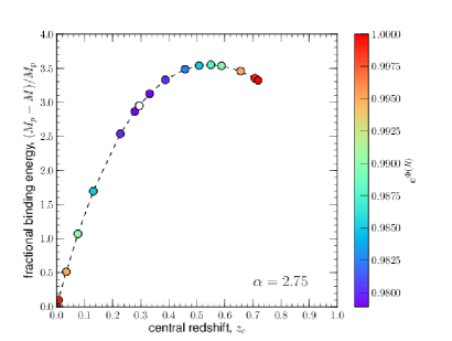
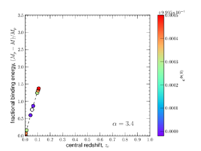
Figure 1: Central redshift-from-rest versus fractional binding energy $f=(M_{p}(R)-M(R))/M_{p}(R)$ for all models with $\alpha=0.5$ (top), $\alpha=2.75$ (middle), and $\alpha=3.4$ (bottom). For $\alpha=0.5$, the effect of different $\beta$-values, between 0.5 and 5.0, is explored. For all other $\alpha$-values, only $\beta=0.5$ was used. The color scale of the data points indicates the value of the potential at the outer boundary of the model, $e^{\Phi}$. The model with the smallest value for $e^{\Phi}$ for each $\alpha$-value is indicated with a white dot in each panel. Models to the left of this white dot have shallower potentials; those to the right of it have deeper potentials.

With which Newtonian model should a given relativistic cluster be compared? A natural choice for the polytropic index is given by (52). From (54), it is obvious that the dimensionless radius $\xi$ can be rescaled to the dimensionless radius $x$ with the scale depending on the central pressure and density. We rescale the density profile such that the total mass equals unity, something we will also do with the relativistic models, giving us a value for $\rho_{c}$. We then adopt a value for the constant $K$ such that $P_{c}=K\rho_{c}^{1+\frac{1}{n}}$. In this case, $2\psi(R)/c^{2}=-1/{\cal A}X$ with $X=R/a$ the dimensionless outer boundary of the Newtonian cluster (which, obviously, does not need to coincide with the outer boundary of the relativistic cluster).

One further remark concerns the fact that in the case of Newtonian stellar clusters, one can choose the mass-scale $M$ and the length-scale $a$ independently from each other whereas in the general relativistic models presented here these two parameters are linked by the parameter $\cal A$, defined as (28), and they cannot be chosen freely. However, in the Newtonian limit, which can be defined formally as the limit $c\rightarrow\infty$, the parameter $1/{\cal A}$ goes to zero,

$$\lim_{c\rightarrow\infty}\frac{1}{\cal A}=\lim_{c\rightarrow\infty}\frac{2GM}{c^{2}a}=0,$$ (56)

for a finite mass-scale $M$ and non-zero length-scale $a$. In that limit, $M$ and $a$ are effectively decoupled since $1/\cal A$ is always zero, irrespective of which mass and length-scale one chooses.

3 Solving the field equations

The two relevant field equations, as shown in e.g. Occhionero & San Martini (1974), are

$$\frac{dM}{dr}(r) =4\pi r^{2}\rho$$ (57)

$$\frac{d\phi}{dr}(r) =\frac{2G}{c^{2}r^{2}}\left[M(r)+4\pi r^{3}\frac{P}{c^{2}}\right]\left[1-\frac{2GM(r)}{rc^{2}}\right]^{-1}.$$ (58)

If we denote the dimensionless radius by $x=r/a$, the scaled mass by ${\cal M}(r)=M(r)/M$, the scaled density by $\tilde{\rho}=\rho a^{3}/M$, and the scaled pressure by $\tilde{P}=Pa^{3}/Mc^{2}$, we can rewrite these equations in a fully dimensionless form as

$$\frac{d{\cal M}}{dx} =4\pi x^{2}\tilde{\rho}$$ (59)

$$\frac{d\phi}{dx} =\frac{1}{{\cal A}x^{2}}\left[{\cal M}+4\pi x^{3}\tilde{P}\right]\left[1-\frac{\cal M}{{\cal A}x}\right]^{-1}.$$ (60)

These equations must be integrated numerically starting from the initial conditions

$${\cal M}(0) =0,$$

$$\phi(0) =\phi_{0}$$ (61)

where $\phi_{0}$ must be chosen such that

$$\exp(\phi(X))=\exp(\Phi)=1-\frac{{\cal M}(X)}{{\cal A}X},$$ (62)

with $X=R/a$ the scaled radius at the cluster’s outer boundary. This ensures that the “internal” solution smoothly goes over into the “external” Schwarzschild solution. This precludes the retrieval of infinitely extended models, especially if they have a diverging mass.

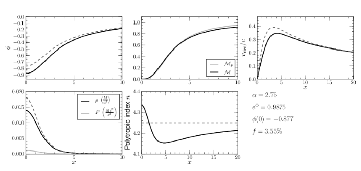
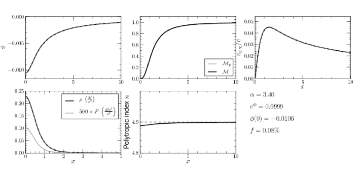
Figure 2: The potential, $\phi$, gravitating and proper mass profiles, ${\cal M}$ and ${\cal M}_{p}$, circular-velocity profile, $v_{\sf circ}$, density $\rho$ and pressure $P$ profiles, and effective polytropic index $n$ for models with $\alpha=0.5$, 2.75, and 3.4. Where visible, the vertical line indicates the outer boundary of the cluster model. The dashed curves indicate the circular-velocity profile, density profile, and polytropic index of the corresponding Newtonian cluster with the same total gravitating mass and the same central pressure. For each model, its values for $\alpha$, the boundary potential $e^{\Phi}$, the central potential $\phi(0)$, and the fractional binding energy $f$ are indicated. All models have $\beta=1/2$.

By explicitly pulling out the $\cal A$-dependence of the density and pressure, it becomes clear that by rescaling the mass and radius according to

$$x^{\prime} ={\cal A}^{(1+2\alpha)/4}x$$ (63)

$${\cal M}^{\prime} ={\cal A}^{(2\alpha-3)/4}{\cal M},$$ (64)

the parameter $\cal A$ can be completely removed from the dimensionless field equations. So one can always set ${\cal A}=1$ in the field equations, solve them, and then afterwards rescale to that particular value of ${\cal A}$ for which ${\cal M}(X)=1$. In that case, the mass scale $M$ equals the total gravitating mass of the cluster and ${\cal A}$ has the meaning of the ratio of $a$ to $R_{S}$.

We wrote a small Python program to numerically integrate these equations and to determine the central value of the potential using a least squares minimizer.

4 Discussion

4.1 Existence of solutions

For each choice of $\alpha$, the only free parameter in the field equations is the value of the potential at the outer boundary of the cluster, in the form $e^{\Phi}$. Our numerical work shows that the field equations presented in the previous section have a bifurcation at some $\alpha$-dependent critical value, $e^{\Phi_{0}(\alpha)}$. For $e^{\Phi}<e^{\Phi_{0}(\alpha)}$, no solutions exist. At $e^{\Phi}=e^{\Phi_{0}(\alpha)}$, a single solution appears. For choices $1\geq e^{\Phi}>e^{\Phi_{0}(\alpha)}$, two solutions, with different central potential values $\phi_{0}$, exist. This can be seen in Fig. 1 in which the fractional binding energy $f$ is plotted versus the central redshift-from-rest $z_{c}$ for models with $\alpha=0.5$, 2.75, and 3.4. We always adopt the value $\beta=1/2$ except in the top panel, where the effects of different $\beta$-values are explored. In each panel, the model with the smallest value for $e^{\Phi}$ is indicated by a white dot. The color of the other data points corresponds to their $e^{\Phi}$-value, as indicated by the colorbar. To the left of the white dot are models with shallower potential wells with the Newtonian $f=0$, $z_{c}=0$ model as limit. To the right of the white dot are models with deeper potential wells and correspondingly higher central redshifts. This situation is reminiscent to that of the family of models discussed by Bisnovatyi-Kogan et al. (1998) which also exhibits both bifurcations (i.e. more than one solution for a given set of model parameters) and limiting values for a parameter connected to the energy at the outer boundary.

For small values for the power $\alpha$, below $\alpha\sim 3$, the $f-z_{c}$-curve has a maximum around $z_{c}\approx 0.5$. As $\alpha$ increases, the right side of the $f-z_{c}$-curve appears to curl up from right to left until this maximum disappears and the $f-z_{c}$-relation is monotonically rising. In the limit $\alpha\rightarrow 7/2$, only the Newtonian $f=0$, $z_{c}=0$ model exists. This means that the Plummer model is a purely Newtonian construct: no relativistic models with $\alpha=7/2$ exist. Also in the Newtonian is the Plummer model a limiting case. As the polytropic index $n$ is increased from zero, it is the first solution of the Lane-Emden equation with infinite extent. It is also the last model with a finite total mass. This appears also to be true relativistically. By construction we are searching for models with a finite total mass by trying to match the solutions of the field equations to an external Schwarzschild metric. No such solutions exist for $\alpha>7/2$.

This is true for different values of the power $\beta$. However, increasing $\beta$ shifts the high-$z_{c}$ end of the $f-z_{c}$-relation in the direction of smaller $z_{c}$, i.e. towards models with shallower potentials. An increase of $\beta$ also raises the $e^{\Phi}$-value of those most relativistic cluster models which means they become less compact (see paragraph 4.4).

The general conclusion we can draw from this is that the steeper the distribution function $F(E)$ varies as a function of energy $E$, the more the solutions are confined towards the Newtonian limit $(f=0,z_{c}=0)$ and that no relativistic models with finite mass exist with $\alpha>7/2$.

4.2 Model properties

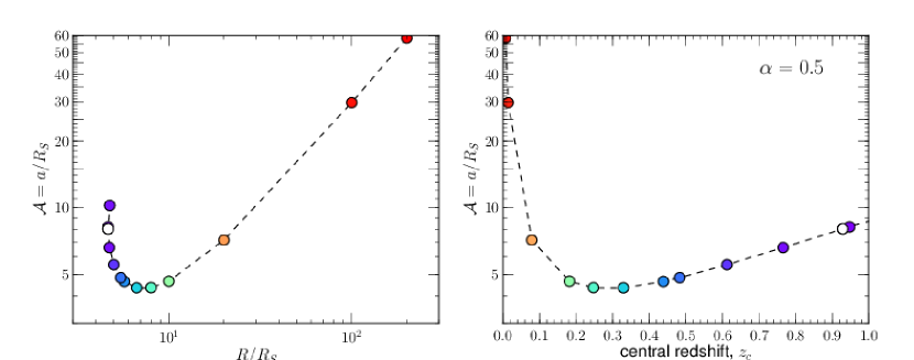
Figure 3: The ratio of the scale radius to the Schwarzschild radius, ${\cal A}=a/R_{S}$ versus outer boundary radius $R/R_{S}$ (left panel) and the central redshift-from-rest $z_{c}$ (right panel) for the models with $\alpha=\beta=0.5$. The color scale of the data points indicates the value of the potential at the outer boundary of the model, $e^{\Phi}$.

In Fig. 2, we present the potential function $\phi$, the gravitating and proper mass profiles, ${\cal M}$ and ${\cal M}_{p}$, the circular-velocity profile, $v_{\sf circ}$, the density $\rho$ and pressure $P$ profiles, and the effective polytropic index $n$ for models with $\alpha=0.5$, 2.75, and 3.4. For all models, we adopt $\beta=1/2$. The dashed curves indicate the circular-velocity profile, density profile, and polytropic index of the corresponding Newtonian cluster with the same total gravitating mass and the same central pressure. The effective polytropic index $n$ is here defined as

$$1+\frac{1}{n}=\frac{d\ln P}{d\ln\rho}$$ (65)

which can be compared with the index (52) derived from the power $\alpha$ in the expression for the distribution function. In the Newtonian limit, both indices coincide.

The $\alpha=3.4$ model shown in Fig. 2 has a very shallow potential and is essentially Newtonian. Therefore, it is indistinguishable from the Newtonian solution of the Lane-Emden equation. The models with $\alpha=0.5$ and $\alpha=2.75$ have much deeper gravitational wells and are well in the general relativistic regime. Clearly, these models do not have polytropic equations of state and their effective polytropic indices can differ significantly from the value expected from their $\alpha$-value. For the same total mass, their density profiles are less steep than those of the Newtonian models. This, combined with the gravitational time dilatation effect in eqn. (39) for the circular velocity, causes the relativistic circular-velocity curve to be much flatter than its Newtonian counterpart.

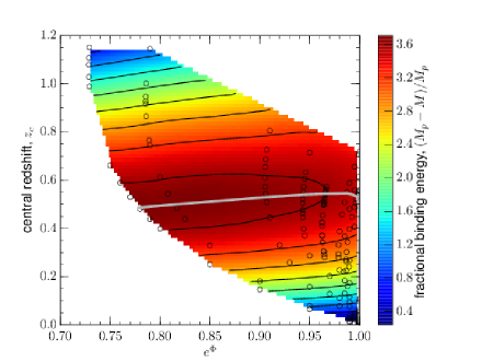
Figure 4: The fractional binding energy $f=(M_{p}(R)-M(R))/M_{p}(R)$ as a function of central redshift $z_{c}$ and the potential at the outer edge of the mass distribution, quantified by $\exp(\Phi)$. The color scale measures $f$ in percentages; the open circles indicate the positions of the models that were actually constructed. The different model sequences have different values for the power $\alpha$.

The ratio of the scale-length to the Schwarzschild radius, quantified by ${\cal A}=a/R_{S}$, is plotted as a function of the ratio of the outer boundary radius to the Schwarzschild radius, $R/R_{S}$, and of the central redshift-from-rest, $z_{c}$, in Fig. 3 for the $\alpha=\beta=0.5$ models. $a/R_{S}$ shows a non-trivial behavior in the sense that the model with the smallest scale-length is neither the most tightly bound model (the one with the largest fractional binding energy $f$) nor the most compact one (the one with the smallest $e^{\Phi}$ or $R/R_{S}$ value). $a/R_{S}$ diverges for $z_{c}\rightarrow 0$ since the Schwarzschild radius tends to zero in the Newtonian limit. In the limit of extremely compact models, $a/R_{S}$ increases again. Apparently, only models with very flat-topped density profiles, with $a\gtrsim R$, can exist in this regime.

4.3 Binding energy

We plot the fractional binding energy $f=(M_{p}(R)-M(R))/M_{p}(R)$ as a function of central redshift $z_{c}$ and the potential at the outer edge of the mass distribution, quantified by $\exp(\Phi)$, in Fig. 4. The open circles in this figure indicate the loci of the models that were actually constructed. The different model sequences have different values for the power $\alpha$, the leftmost corresponding to $\alpha=0.05$. The 2D map of the binding energy was constructed by applying a bicubic spline interpolator to the model points. The models nicely cover the first maximum of $f$, where dynamical instability is expected to set in (Bisnovatyi-Kogan et al., 1998; Bisnovatyi-Kogan & Merafina, 2006).

The grey line connects the models which, for a given $\alpha$, attain the maximum fractional binding energy. The models with $\alpha$ in the range $0.05$ to $\approx 3.0$ have central redshift-from-rest values between $\approx 0.5$ and $\approx 0.55$. For higher $\alpha$-values, the maximum central redshift rapidly drops to zero. As the power $\alpha$ approaches the value of 7/2, the Plummer model value, both the central redshift-from-rest and the fractional binding energy go to zero, the Newtonian limit. The overall maximum central redshift-from-rest is achieved by the model with $\alpha=2.75$.

This behavior is caused by the $\alpha$-dependence of the shape of the $f-z_{c}$-relation which was discussed in paragraph 4.1. At first, steepening the distribution function by increasing $\alpha$ above zero leads to a deepening of the potential well and therefore to a slight increase of $z_{c}$. Above $\alpha\approx 2.75$, a further steepening of the distribution function and of the density profile limits the models more and more to the Newtonian limit, thus reducing $z_{c}$.

4.4 The radius

Each model is labelled by a unique $\cal A$-value for which the mass scale $M$ coincides with the model’s total mass. If we select this particular value for $\cal A$ or, equivalently, $M$ , the quantity

$$R_{S}=\frac{2GM}{c^{2}}$$ (66)

has the physical meaning of being the model’s Schwarzschild radius. Numerically integrating the field equations yields the dimensionless outer radius $X$. Multiplying this radius with the scale-length $a$ gives the physical value for the radius $R=aX$. It then follows that

$$\frac{1}{\cal A}=\frac{2GM}{c^{2}a}=\frac{2GM}{c^{2}R}X$$ (67)

and consequently

$$\frac{R}{R_{S}}={\cal A}X=\frac{1}{1-\exp(\Phi)},$$ (68)

where we made use of eqn. (62).

For each value of $\alpha$, there exists a minimum value for $\Phi$ below which no solutions to the field equations can be found. Using the above, this corresponds to a minimum value for $R/R_{S}$. As $\alpha$ tends to zero, the minimum radius shrinks to $R\approx 3.6R_{S}$, as can be seen in Fig. 5. Hence, models with very “flat” distribution functions and density and pressure profiles can be very small, with radii only a few times larger than their Schwarzschild radius. As the distribution function and the corresponding density and pressure profiles are steepened by increasing the value of the power $\alpha$, this minimum radius steadily increases. In the limit $\alpha\rightarrow 7/2$ the only possible solution is the Newtonian Plummer model and the minimum radius grows to infinity.

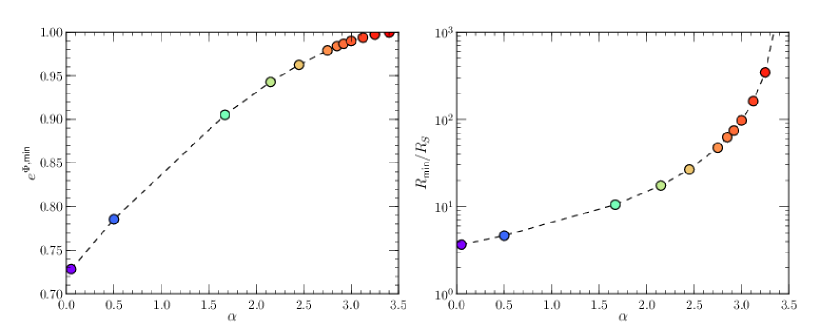
Figure 5: The minimum value for $e^{\Phi}$ versus $\alpha$ (left) and the smallest possible radius, divided by the model’s Schwarzschild radius versus $\alpha$ (right).

5 Conclusions

We show that the equations underlying the general relativistic theory of spherically symmetric isotropic stellar clusters can be cast in a form analogous to that of the Newtonian theory. Using the mathematical formalism developed for the latter, we prove that the distribution function can be derived from any isotropic momentum moment $\tilde{\mu}_{k,2q}$. This is a direct generalization of the inversion relations derived by Fackerell (1968) and Pogorelov & Kandrup (1996). Moreover, every higher-order moment $\tilde{\mu}_{k,2q}$, with $q>0$, can be written as an integral over the corresponding zeroth-order moment $\tilde{\mu}_{k,0}$.

We propose a mathematically simple expression for the distribution function of a family of isotropic cluster models which is guaranteed to be positive everywhere in phase space. The distribution function of each model is basically defined by two parameters: the slope $\alpha$ and the value of the potential at the boundary, $\Phi$. In the Newtonian limit, these models reduce to the family of polytropic models. In the relativistic regime, however, these models do not have a polytropic equation of state. We derive the Newtonian limits of the general equations underlying the cluster dynamics and the density and pressure profiles of the polytropic cluster models.

For a given $\alpha$, the field equations for these general relativistic cluster models only allow solutions if $\Phi>\Phi_{0}(\alpha)$, with $\Phi_{0}(\alpha)$ an $\alpha$-dependent minimum value for the potential at the outer boundary. In other words: for a given slope of the distribution function, a model cannot be made arbitrarily compact. The ratio of the minimum outer radius to the model’s Schwarzschild radius is a rising function of $\alpha$, increasing from $R/R_{S}\approx 3.6$ for $\alpha=0$ to $R/R_{s}=\infty$ for $\alpha=3.5$. For less compact models, always two solutions to the field equations exist: one with a higher central redshift than the most compact model and one with a lower central redshift.

The models we constructed, for $\alpha$-values between $0.05$ and $3.5$, fully cover the first maximum of the fractional binding, where dynamical instability is expected to set in. This first maximum is achieved by models which all have a central redshift below $z_{c}\approx 0.55$. The most strongly bound model is characterized by $\alpha=2.75$ and a central redshift $z_{c}\approx 0.55$. Models with steeper distribution functions have lower fractional binding energies than the $\alpha=2.75$ model whereas models with flatter distribution functions have higher fractional binding energies. In the limit $\alpha\rightarrow 3.5$, the binding energy and the central redshift both tend to zero. This indicates that in this limit the distribution function has become too steep to allow for anything but the Newtonian solution: no models with a finite mass exist for $\alpha>3.5$. Hence, we can conclude that, at least within the context of this family of models, the Plummer model by necessity is a purely Newtonian construct.

References

- Bisnovatyi-Kogan et al. (1998) Bisnovatyi-Kogan G. S., Merafina M., Ruffini R., Vesperini E., 1998, ApJ, 500, 217-232
- Bisnovatyi-Kogan & Merafina (2006) Bisnovatyi-Kogan G. S. & Merafina M., 2006, ApJ, 653, 1445-1453
- Buchdahl (1964) Buchdahl H. A., 1964, ApJ, 140, 1512-1516
- Dejonghe (1986) Dejonghe H., 1986, Physics Reports, Vol. 133, No. 3-4, 217-313
- Dejonghe (1987) Dejonghe H., 1987, MNRAS, 224, 13-39
- Eddington (1916) Eddington A. S., 1916, MNRAS, 76, 572-585
- Fackerell (1968) Fackerell E. D., 1968, ApJ, 153, 643-660
- Fackerell (1969) Fackerell E. D., 1969, CoASP, 1, 134-139
- Fackerell (1971) Fackerell E. D., 1971, ApJ, 165, 489-493
- Ipser (1969) Ipser J. R., 1969, ApJ, 158, 17-44
- Kaufmann (1967) Kaufmann W. J., iii, 1967, AJ, 72, 754-756
- Merafina & Ruffini (1995) Merafina M. & Ruffini R., 1995, ApJ, 454, L89-L92
- Nguyen & Lingam (2013) Nguyen P. H. & Lingam M., 2013, MNRAS, 436, 2014-2028
- Occhionero & San Martini (1974) Occhionero F. & San Martini A., 1974, A&A, 32, 203-208
- Plummer (1911) Plummer H. C., 1911, MNRAS, 71, 460-470
- Pogorelov & Kandrup (1996) Pogorelov I. V. & Kandrup H. E., 1996, Phys. Rev. E, 53, 1375-1381
- Rasio, Shapiro, Teukolsky (1989) Rasio F. A., Shapiro S. L., Teukolsky S. A., 1989, ApJ, 336, L63-L66
- Shapiro & Teukolsky (1985) Shapiro S. L. & Teukolsky S. A., 1985, ApJ, 298, 58-79
- Suffern (1977) Suffern K. G., 1977, J. Phys. A, 10, 1897-1903
- Tooper (1964) Tooper R. F., 1964, ApJ, 140, 434-459