Blow-up results for a strongly perturbed semilinear heat equation: Theoretical analysis and numerical method

Abstract

We consider a blow-up solution for a strongly perturbed semilinear heat equation with Sobolev subcritical power nonlinearity. Working in the framework of similarity variables, we find a Lyapunov functional for the problem. Using this Lyapunov functional, we derive the blow-up rate and the blow-up limit of the solution. We also classify all asymptotic behaviors of the solution at the singularity and give precisely blow-up profiles corresponding to these behaviors. Finally, we attain the blow-up profile numerically, thanks to a new mesh-refinement algorithm inspired by the rescaling method of Berger and Kohn [5]. Note that our method is applicable to more general equations, in particular those with no scaling invariance.

Keywords: Blow-up, Lyapunov functional, asymptotic behavior, blow-up profile, semilinear heat equation, lower order term.

1 Introduction

We are concerned in this paper with blow-up phenomena arising in the following nonlinear heat problem:

$$\left\{\begin{array}[]{rcl}u_{t}&=&\Delta u+|u|^{p-1}u+h(u),\\ u(.,0)&=&u_{0}\in L^{\infty}(\mathbb{R}^{n}),\end{array}\right.$$ (1)

where $u(t):x\in\mathbb{R}^{n}\to u(x,t)\in\mathbb{R}$ and $\Delta$ stands for the Laplacian in $\mathbb{R}^{n}$. The exponent $p>1$ is subcritical (that means that $p<\frac{n+2}{n-2}$ if $n\geq 3$) and $h$ is given by

$$h(z)=\mu\dfrac{|z|^{p-1}z}{\log^{a}(2+z^{2})},\quad\text{with}\;\;a>0,\;\mu\in\mathbb{R}.$$ (2)

By standard results, the problem (1) has a unique classical solution $u(x,t)$ in $L^{\infty}(\mathbb{R}^{n})$, which exists at least for small times. The solution $u(x,t)$ may develop singularities in some finite time. We say that $u(x,t)$ blows up in a finite time $T$ if $u(x,t)$ satisfies (1) in $\mathbb{R}^{b}\times[0,T)$ and

$$\lim_{t\to T}\|u(t)\|_{L^{\infty}(\mathbb{R}^{n})}=+\infty.$$

$T$ is called the blow-up time of $u(x,t)$. In such a blow-up case, a point $b\in\mathbb{R}^{n}$ is called a blow-up point of $u(x,t)$ if and only if there exist $(x_{n},t_{n})\to(b,T)$ such that $|u(x_{n},t_{n})|\to+\infty$ as $n\to+\infty$.

In the case $\mu=0$, the equation (1) is the semilinear heat equation,

$$u_{t}=\Delta u+|u|^{p-1}u.$$ (3)

Problem (3) has been addressed in different ways in the literature. The existence of blow-up solutions has been proved by several authors (see Fujita [12], Levine [27], Ball [3]). Consider $u(x,t)$ a solution of (3) which blows up at a time $T$. The very first question to be answered is the blow-up rate, i.e. there are positive constants $C_{1},C_{2}$ such that

$$C_{1}(T-t)^{-\frac{1}{p-1}}\leq\|u(t)\|_{L^{\infty}(\mathbb{R}^{n})}\leq C_{2}(T-t)^{-\frac{1}{p-1}},\quad\forall t\in(0,T).$$ (4)

The lower bound in (4) follows by a simple argument based on Duhamel’s formula (see Weissler [36]). For the upper bound, Giga and Kohn proved (4) in [13] for $1<p<\frac{3n+8}{3n-4}$ or for non-negative initial data with subcritical $p$. Then, this result was extended to all subcritiacal $p$ without assuming non-negativity for initial data $u_{0}$ by Giga, Matsui and Sasayama in [15]. The estimate (4) is a fundamental step to obtain more information about the asymptotic blow-up behavior, locally near a given blow-up point $\hat{b}$. Giga and Kohn showed in [14] that for a given blow-up point $\hat{b}\in\mathbb{R}^{n}$,

$$\lim_{t\to T}(T-t)^{\frac{1}{p-1}}u(\hat{b}+y\sqrt{T-t},t)=\pm\kappa,$$

where $\kappa=(p-1)^{-\frac{1}{p-1}}$, uniformly on compact sets of $\mathbb{R}^{n}$.
This result was specified by Filippas ans Liu [11] (see also Filippas and Kohn [10]) and Velázquez [34], [35] (see also Herrero and Velázquez [22], [24], [21]). Using the renormalization theory, Bricmont and Kupiainen showed in [6] the existence of a solution of (3) such that

$$\left\|(T-t)^{\frac{1}{p-1}}u(\hat{b}+z\sqrt{(T-t)|\log(T-t)|},t)-f_{0}(z)\right\|_{L^{\infty}(\mathbb{R}^{n})}\to 0\quad\text{as}\quad t\to T,$$ (5)

where

$$f_{0}(z)=\kappa\left(1+\frac{p-1}{4p}|z|^{2}\right)^{-\frac{1}{p-1}}.$$ (6)

Merle and Zaag in [29] obtained the same result through a reduction to a finite dimensional problem. Moreover, they showed that the profile (6) is stable under perturbations of initial data (see also [8], [9] and [28]).

In the case where the function $h$ satisfies

$$j=0,1,\;\;|h^{(j)}(z)|\leq M\left(\frac{|z|^{p-j}}{\log^{a}(2+z^{2})}+1\right),\quad|h^{\prime\prime}(z)|\leq M\frac{|z|^{p-2}}{\log^{a}(2+z^{2})},$$ (7)

with $a>1$ and $M>0$, we proved in [32] the existence of a Lyapunov functional in similarity variables for the problem (1) which is a crucial step in deriving the estimate (4). We also gave a classification of possible blow-up behaviors of the solution when it approaches to singularity. In [33], we constructed a blow-up solution of the problem (1) satisfying the behavior described in (5) in the case where $h$ satisfies the first estimate in (7) or $h$ is given by (2).

In this paper, we aim at extending the results of [32] to the case $a\in(0,1]$. As we mentioned above, the first step is to derive the blow-up rate of the blow-up solution. As in [15] and [32], the key step is to find a Lyapunov functional in similarity variables for equation (1). More precisely, we introduce for all $b\in\mathbb{R}^{n}$ ($b$ may be a blow-up point of $u$ or not) the following similarity variables:

$$y=\frac{x-b}{\sqrt{T-t}},\quad s=-\log(T-t),\quad w_{b,T}=(T-t)^{\frac{1}{p-1}}u(x,t).$$ (8)

Hence $w_{b,T}$ satisfies for all $s\geq-\log{T}$ and for all $y\in\mathbb{R}^{n}$:

$$\partial_{s}w_{b,T}=\frac{1}{\rho}\text{div}(\rho\nabla w_{b,T})-\frac{w_{b,T}}{p-1}+|w_{b,T}|^{p-1}w_{b,T}+e^{-\frac{ps}{p-1}}h\left(e^{\frac{s}{p-1}}w_{b,T}\right),$$ (9)

where

$$\rho(y)=\left(\frac{1}{4\pi}\right)^{n/2}e^{-\frac{|y|^{2}}{4}}.$$ (10)

Following the method introduced by Hamza and Zaag in [19], [20] for perturbations of the semilinear wave equation, we introduce

$$\mathcal{J}_{a}[w](s)=\mathcal{E}[w](s)e^{\frac{\gamma}{a}s^{-a}}+\theta s^{-a},$$ (11)

where $\gamma$, $\theta$ are positive constants depending only on $p$, $a$, $\mu$ and $n$ which will be determined later, and

$$\mathcal{E}[w]=\mathcal{E}_{0}[w]+\mathcal{I}[w],$$ (12)

where

$$\mathcal{E}_{0}[w](s)=\int_{\mathbb{R}^{n}}\left(\frac{1}{2}|\nabla w|^{2}+\frac{1}{2(p-1)}|w|^{2}-\frac{1}{p+1}|w|^{p+1}\right)\rho dy,$$ (13)

and

$$\mathcal{I}[w](s)=-e^{-\frac{p+1}{p-1}s}\int_{\mathbb{R}^{n}}H\left(e^{\frac{s}{p-1}}w\right)\rho dy,\;\;H(z)=\int_{0}^{z}h(\xi)d\xi.$$ (14)

The main novelty of this paper is to allow values of $a$ in $(0,1]$, and this is possible at the expense of taking the particular form (2) for the perturbation $h$. We aim at the following:

Theorem 1 (Existence of a Lyapunov functional for equation (9)).

Let $a,p,n,\mu$ be fixed, consider $w$ a solution of equation (9). Then, there exist $\hat{s}_{0}=\hat{s}_{0}(a,p,n,\mu)\geq s_{0}$, $\hat{\theta}_{0}=\hat{\theta}_{0}(a,p,n,\mu)$ and $\gamma=\gamma(a,p,n,\mu)$ such that if $\theta\geq\hat{\theta}_{0}$, then $\mathcal{J}_{a}$ satisfies the following inequality, for all $s_{2}>s_{1}\geq\max\{\hat{s}_{0},-\log T\}$,

$$\mathcal{J}_{a}[w](s_{2})-\mathcal{J}_{a}[w](s_{1})\leq-\frac{1}{2}\int_{s_{1}}^{s_{2}}\int_{\mathbb{R}^{n}}(\partial_{s}w)^{2}\rho dyds.$$ (15)

As in [15] and [32], the existence of the Lyapunov functional is a crucial step for deriving the blow-up rate (4) and then the blow-up limit. In particular, we have the following:

Theorem 2.

Let $a,p,n,\mu$ be fixed and $u$ be a blow-up solution of equation (1) with a blow-up time $T$.
$(i)\;$ (Blow-up rate) There exists $\hat{s}_{1}=\hat{s}_{1}(a,p,n,\mu)\geq\hat{s}_{0}$ such that for all $s\geq s^{\prime}=\max\{\hat{s}_{1},-\log T\}$,

$$\|w_{b,T}(y,s)\|_{L^{\infty}(\mathbb{R}^{n})}\leq C,$$ (16)

where $w_{b,T}$ is defined in (8) and $C$ is a positive constant depending only on $n,p,\mu$ and a bound of $\|w_{b,T}(\hat{s}_{0})\|_{L^{\infty}}$.
$(ii)\;$ (Blow-up limit) If $\hat{a}$ is a blow-up point, then

$$\lim_{t\to T}(T-t)^{\frac{1}{p-1}}u(\hat{a}+y\sqrt{T-t},t)=\lim_{s\to+\infty}\,w_{\hat{a},T}(y,s)=\pm\kappa,$$ (17)

holds in $L^{2}_{\rho}$ ($L^{2}_{\rho}$ is the weighted $L^{2}$ space associated with the weight $\rho$ (10)), and also uniformly on each compact subset of $\mathbb{R}^{n}$.

Remark 1.

We will not give the proof of Theorem 2 because its proof follows from Theorem 1 as in [32]. Hence, we only give the proof of Theorem 1 and refer the reader to Section 2 in [32] for the proofs of (16) and (17) respectively.

The next step consists in obtaining an additional term in the asymptotic expansion given in $(ii)$ of Theorem 2. Given $b$ a blow-up point of $u(x,t)$, and up to changing $u_{0}$ by $-u_{0}$ and $h$ by $-h$, we may assume that $w_{b,T}\to\kappa$ in $L^{2}_{\rho}$ as $s\to+\infty$. As in [32], we linearize $w_{b,T}$ around $\phi$, where $\phi$ is the positive solution of the ordinary differential equation associated to (9),

$$\phi_{s}=-\frac{\phi}{p-1}+\phi^{p}+e^{-\frac{ps}{p-1}}h\left(e^{\frac{s}{p-1}}\phi\right)$$ (18)

such that

$$\phi(s)\to\kappa\quad\text{as}\quad s\to+\infty,$$ (19)

(see Lemma A.3 in [32] for the existence of $\phi$, and note that $\phi$ is unique. For the reader’s convenience, we give in Lemma A.1 the expansion of $\phi$ as $s\to+\infty$).

Let us introduce $v_{b,T}=w_{b,T}-\phi(s)$, then $\|v_{b,T}(y,s)\|_{L^{2}_{\rho}}\to 0$ as $s\to+\infty$ and $v_{b,T}$ (or $v$ for simplicity) satisfies the following equation:

$$\partial_{s}v=(\mathcal{L}+\omega(s))v+F(v)+H(v,s),\quad\forall y\in\mathbb{R}^{n},\;\forall s\in[-\log T,+\infty),$$

where $\mathcal{L}=\Delta-\frac{y}{2}\cdot\nabla+1$ and $\omega$, $F$, $H$ satisfy

$$\omega(s)=\mathcal{O}(\frac{1}{s^{a+1}})\quad\text{and}\quad|F(v)|+|H(v,s)|=\mathcal{O}(|v|^{2})\quad\text{as $s\to+\infty$},$$

(see the beginning of Section 3 for the proper definitions of $\omega$, $F$ and $G$).
It is well known that the operator $\mathcal{L}$ is self-adjoint in $L^{2}_{\rho}(\mathbb{R}^{n})$. Its spectrum is given by

$$spec(\mathcal{L})=\{1-\frac{m}{2},\;m\in\mathbb{N}\},$$

and it consists of eigenvalues. The eigenfunctions of $\mathcal{L}$ are derived from Hermite polynomials:
- For $n=1$, the eigenfunction corresponding to $1-\frac{m}{2}$ is

$$h_{m}(y)=\sum_{k=0}^{\left[\frac{m}{2}\right]}\frac{m!}{k!(m-2k)!}(-1)^{k}y^{m-2k},$$ (20)

- For $n\geq 2$: we write the spectrum of $\mathcal{L}$ as

$$spec(\mathcal{L})=\{1-\frac{|m|}{2},\;|m|=m_{1}+\dots+m_{n},\;(m_{1},\dots,m_{n})\in\mathbb{N}^{n}\}.$$

For $m=(m_{1},\dots,m_{n})\in\mathbb{N}^{n}$, the eigenfunction corresponding to $1-\frac{|m|}{2}$ is

$$H_{m}(y)=h_{m_{1}}(y_{1})\dots h_{m_{n}}(y_{n}),$$ (21)

where $h_{m}$ is defined in (20).
We also denote $c_{m}=c_{m_{1}}c_{m_{2}}\dots c_{m_{n}}$ and $y^{m}=y_{1}^{m_{1}}y_{2}^{m_{2}}\dots y_{n}^{m_{n}}$ for any $m=(m_{1},\dots,m_{n})\in\mathbb{N}^{n}$ and $y=(y_{1},\dots,y_{n})\in\mathbb{R}^{n}$.
By this way, we derive the following asymptotic behaviors of $w_{b,T}(y,s)$ as $s\to+\infty$:

Theorem 3 (Classification of the behavior of $w_{b,T}$ as $s\to+\infty$).

Consider $u(t)$ a solution of equation (1) which blows-up at time $T$ and $b$ a blow-up point. Let $w_{b,T}(y,s)$ be a solution of equation (9). Then one of the following possibilities occurs:
$i)\;$ $w_{b,T}(y,s)\equiv\phi(s)$,
$ii)$ There exists $l\in\{1,\dots,n\}$ such that up to an orthogonal transformation of coordinates, we have

$$w_{b,T}(y,s)=\phi(s)-\frac{\kappa}{4ps}\left(\sum_{j=1}^{l}y_{j}^{2}-2l\right)+\mathcal{O}\left(\frac{1}{s^{a+1}}\right)+\mathcal{O}\left(\frac{\log s}{s^{2}}\right)\quad\text{as}\quad s\to+\infty,$$

$iii)$ There exist an integer number $m\geq 3$ and constants $c_{\alpha}$ not all zero such that

$$w_{b,T}(y,s)=\phi(s)-e^{-\left(\frac{m}{2}-1\right)s}\sum_{|\alpha|=m}c_{\alpha}H_{\alpha}(y)+o\left(e^{-\left(\frac{m}{2}-1\right)s}\right)\quad\text{as}\quad s\to+\infty.$$

The convergence takes place in $L^{2}_{\rho}$ as well as in $\mathcal{C}^{k,\gamma}_{loc}$ for any $k\geq 1$ and some $\gamma\in(0,1)$.

Remark 2.

In our previous paper [32], we were unable to get this result in the case where $h$ satisfies (7) with $a\in(0,1]$. Here, by taking the particular form of the perturbation (see (2)), we are able to overcome technical difficulties in order to derive the result.

Remark 3.

From $ii)$ of Theorem 2, we would naturally try to find an equivalent for $w-\kappa$ as $s\to+\infty$. A posteriori from our results in Theorem 3, we see that in all cases $\|w-\kappa\|_{L^{2}_{\rho}}\sim\frac{C}{s^{a^{\prime}}}$ with $a^{\prime}=\max\{a,1\}$. This is indeed a new phenomenon observed in our equation (1), and which is different from the case of the unperturbed semilinear heat equation where either $w-\kappa\equiv 0$, or $\|w-\kappa\|_{L^{2}_{\rho}}\sim\frac{C}{s}$ or $\|w-\kappa\|_{L^{2}_{\rho}}\sim Ce^{(1-m/2)s}$ for some even $m\geq 4$. This shows the originality of our paper. In our case, linearizing around $\kappa$ would keep us trapped in the $\frac{1}{s}$ scale. In order to escape that scale, we forget the explicit function $\kappa$ which is not a solution of equation (9), and linearizing instead around the non-explicit function $\phi$, which happens to be an exact solution of (9). This way, we escape the $\frac{1}{s}$ scale and reach exponentially decreasing order.

Using the information obtained in Theorem 3, we can extend the asymptotic behavior of $w_{b,T}$ to larger regions. Particularly, we have the following:

Theorem 4 (Convergence extension of $w_{b,T}$ to larger regions).

For all $K_{0}>0$,
$i)$ if $ii)$ of Theorem 3 occurs, then

$$\sup_{|\xi|\leq K_{0}}\left|w_{b,T}(\xi\sqrt{s},s)-f_{l}(\xi)\right|=\mathcal{O}\left(\frac{1}{s^{a}}\right)+\mathcal{O}\left(\frac{\log s}{s}\right),\quad\text{as}\quad s\to+\infty,$$ (22)

where

$$\forall\xi\in\mathbb{R}^{n},\quad f_{l}(\xi)=\kappa\left(1+\frac{p-1}{4p}\sum_{j=1}^{l}\xi_{j}^{2}\right)^{-\frac{1}{p-1}},$$ (23)

with $l$ given in $ii)$ of Theorem 3.
$ii)$ if $iii)$ of Theorem 3 occurs, then $m\geq 4$ is even, and

$$\sup_{|\xi|\leq K_{0}}\left|w_{b,T}\left(\xi e^{\left(\frac{1}{2}-\frac{1}{m}\right)s}\right)-\psi_{m}(\xi)\right|\to 0\quad\text{as}\quad s\to+\infty,$$ (24)

where

$$\forall\xi\in\mathbb{R}^{n},\quad\psi_{m}(\xi)=\kappa\left(1+\kappa^{-p}\sum_{|\alpha|=m}c_{\alpha}\xi^{\alpha}\right)^{-\frac{1}{p-1}},$$ (25)

with $c_{\alpha}$ the same as in Theorem 3, and the multilinear for $\sum_{|\alpha|=m}c_{\alpha}\xi^{\alpha}$ is nonnegative.

Remark 4.

As in the unperturbed case ($h\equiv 0$), we expect that (22) is stable (see the previous remarks, particularly the paragraph after (5)), and (24) should correspond to unstable behaviors (the unstable of (24) was proved only in one space dimension by Herrero and Velázquez in [23] and [25]). While remarking numerical simulation for equation (1) in one space dimension (see Section 4.2 below), we see that the numerical solutions exhibit only the behavior (22), we could never obtain the behavior (24). This is probably due to the fact that the behavior (24) is unstable.

At the end of this work, we give numerical confirmations for the asymptotic profile described in Theorem 4. For this purpose, we propose a new mesh-refinement method inspired by the rescaling algorithm of Berger and Kohn [5]. Note that, their method was successful to solve blowing-up problems which are invariant under the following transformation,

$$\forall\gamma>0,\quad\gamma\mapsto u_{\gamma}(\xi,\tau)=\gamma^{\frac{2}{p-1}}u(\gamma\xi,\gamma^{2}\tau).$$ (26)

However, there are a lot of equations whose solutions blow up in finite time but the equation does not satisfy the property (26), one of them is the equation (1) because of the presence of the perturbation term $h$. Although our method is very similar to Berger and Kohn’s algorithm in spirit, it is better in the sense that it can be applied to a larger class of blowing-up problems which do not satisfy the rescaling property (26). Up to our knowledge, there are not many papers on the numerical blow-up profile, apart from the paper of Berger and Kohn [5] (see also [31]), who already obtained numerical results for equation (1) without the perturbation term. For other numerical aspects, there are several studies for (1) in the unperturbed case, see for example, Abia, López-Marcos and Martínez in [2], [1], Groisman and Rossi [17],[18], [16], N’gohisse and Boni [30], Kyza and Makridakis [26], Cangiani et al. [7] and the references therein. There is also the work of Baruch et al. [4] studying standing-ring solutions.

This paper is organized as follows: Section 2 is devoted to the proof of Theorem 1. Theorem 2 follows from Theorem 1. Since all the arguments presented [32] remain valid for the case (7), except the existence of the Lyapunov functional for equation (9) (Theorem 1), we kindly refer the reader to Section 2.3 and 2.4 in [32] for details of the proof. Section 3 deals with results on asymptotic behaviors (Theorem 3 and Theorem 4). In Section 4, we describe the new mesh-refinement method and give some numerical justifications for the theoretical results.

Acknowledgement: The authors are grateful to M. A. Hamza for several helpful conversations pertaining to this work, and especially for giving the idea for the proof of Theorem 1 in this paper.

2 Existence of a Lyapunov functional for equation (9)

In this section, we mainly aim at proving that the functional $\mathcal{J}_{a}$ defined in (11) is a Lyapunov functional for equation (9) (Theorem 1). Note that this functional is far from being trivial and makes our main contribution.

In what follows, we denote by $C$ a generic constant depending only on $a$, $p$, $n$ and $\mu$. We first give the following estimates on the perturbation term appearing in equation (9):

Lemma 5.

Let $h$ be the function defined in (2). For all $\epsilon\in(0,p]$, there exists $C_{0}=C_{0}(a,\mu,p,\epsilon)>0$ and $\bar{s}_{0}=\bar{s}_{0}(a,p,\epsilon)>0$ large enough such that for all $s\geq\bar{s}_{0}$,
$i)$

$$\left|e^{-\frac{ps}{p-1}}h\left(e^{\frac{s}{p-1}}z\right)\right| \leq\frac{C_{0}}{s^{a}}(|z|^{p}+|z|^{p-\epsilon}),$$

$$\text{and}\;\;\left|e^{-\frac{(p+1)s}{p-1}}H\left(e^{\frac{s}{p-1}}z\right)\right| \leq\frac{C_{0}}{s^{a}}(|z|^{p+1}+1),$$

where $H$ is defined in (14).
$ii)$

$$\left|(p+1)e^{-\frac{(p+1)s}{p-1}}H\left(e^{\frac{s}{p-1}}z\right)-e^{-\frac{ps}{p-1}}h\left(e^{\frac{s}{p-1}}z\right)z\right|\leq\frac{C_{0}}{s^{a+1}}(|z|^{p+1}+1).$$

Proof.

Note that $i)$ obviously follows from the following estimate,

$$\forall q>0,b>0,\quad\frac{|z|^{q}}{\log^{b}(2+e^{\frac{2s}{p-1}}z^{2})}\leq\frac{C}{s^{b}}(|z|^{q}+1),\quad\forall s\geq\bar{s}_{0},$$ (27)

where $C=C(b,q)>0$ and $\bar{s}_{0}=\bar{s}_{0}(b,q)>0$.
In order to derive estimate (27), considering the first case $z^{2}e^{\frac{s}{p-1}}\geq 4$, then the case $z^{2}e^{\frac{s}{p-1}}\leq 4$, we would obtain (27).
$ii)$ directly follows from an integration by part and estimate (27). Indeed, we have

$$H(\xi) =\int_{0}^{\xi}h(x)dx=\mu\int_{0}^{\xi}\frac{|x|^{p-1}x}{\log^{a}(2+x^{2})}dx$$

$$=\frac{\mu|\xi|^{p+1}}{(p+1)\log^{a}(2+\xi^{2})}+\frac{2a\mu}{p+1}\int_{0}^{\xi}\frac{|x|^{p+1}x}{(2+x^{2})\log^{a+1}(2+x^{2})}dx.$$

Replacing $\xi$ by $e^{\frac{s}{p-1}}z$ and using (27), we then derive $ii)$. This ends the proof of Lemma 5. ∎

We assert that Theorem 1 is a direct consequence of the following lemma:

Lemma 6.

Let $a,p,n,\mu$ be fixed and $w$ be solution of equation (9). There exists $\tilde{s}_{0}=\tilde{s}_{0}(a,p,n,\mu)\geq s_{0}$ such that the functional of $\mathcal{E}$ defined in (12) satisfies the following inequality, for all $s\geq\max\{\tilde{s}_{0},-\log T\}$,

$$\frac{d}{ds}\mathcal{E}[w](s)\leq-\frac{1}{2}\int_{\mathbb{R}^{n}}w_{s}^{2}\rho dy+\gamma s^{-(a+1)}\mathcal{E}[w](s)+Cs^{-(a+1)},$$ (28)

where $\gamma=\frac{4C_{0}(p+1)}{(p-1)^{2}}$, $C_{0}$ is given in Lemma 5.

Let us first derive Theorem 1 from Lemma 6 and we will prove it later.

Proof of Theorem 1 admitting Lemma 6.

Differentiating the functional $\mathcal{J}$ defined in (11), we obtain

$$\frac{d}{ds}\mathcal{J}_{a}[w](s) =\frac{d}{ds}\left\{\mathcal{E}[w](s)e^{\frac{\gamma}{a}s^{-a}}+\theta s^{-a}\right\}$$

$$=\frac{d}{ds}\mathcal{E}[w](s)e^{\frac{\gamma}{a}s^{-a}}-\gamma s^{-(a+1)}\mathcal{E}[w](s)e^{\frac{\gamma}{a}s^{-a}}-a\theta s^{-(a+1)}$$

$$\leq-\frac{1}{2}e^{\frac{\gamma}{a}s^{-a}}\int_{\mathbb{R}^{n}}w_{s}^{2}\rho dy+\left[Ce^{\frac{\gamma}{a}s^{-a}}-a\theta\right]s^{-(a+1)}\quad\text{(use \eqref{equ:estimateDE}).}$$

Choosing $\theta$ large enough such that $Ce^{\frac{\gamma}{a}{\tilde{s}_{0}}^{-a}}-a\theta\leq 0$ and noticing that $e^{\frac{\gamma}{a}s^{-a}}\geq 1$ for all $s>0$, we derive

$$\frac{d}{ds}\mathcal{J}_{a}[w](s)\leq-\frac{1}{2}\int_{\mathbb{R}^{n}}w_{s}^{2}\rho dy,\quad\forall s\geq\tilde{s}_{0}.$$

This implies inequality (15) and concludes the proof of Theorem 1, assuming that Lemma 6 holds. ∎

It remains to prove Lemma 6 in order to conclude the proof of Theorem 1.

Proof of Lemma 6 .

Multiplying equation (9) with $w_{s}\rho$ and integrating by parts:

$$\int_{\mathbb{R}^{n}}|w_{s}|^{2}\rho=-\frac{d}{ds}\left\{\int_{\mathbb{R}^{n}}\left(\frac{1}{2}|\nabla w|^{2}+\frac{1}{2(p-1)}|w|^{2}-\frac{1}{p+1}|w|^{p+1}\right)\rho dy\right\}$$

$$+e^{-\frac{ps}{p-1}}\int_{\mathbb{R}^{n}}h\left(e^{\frac{s}{p-1}}w\right)w_{s}\rho dy$$ .

For the last term of the above expression, we write in the following:

$$e^{-\frac{ps}{p-1}}\int_{\mathbb{R}^{n}}h\left(e^{\frac{s}{p-1}}w\right)w_{s}\rho dy=e^{-\frac{(p+1)s}{p-1}}\int_{\mathbb{R}^{n}}h\left(e^{\frac{s}{p-1}}w\right)\left(e^{\frac{s}{p-1}}w_{s}+\frac{e^{\frac{s}{p-1}}}{p-1}w\right)\rho dy$$

$$-\frac{1}{p-1}e^{-\frac{ps}{p-1}}\int_{\mathbb{R}^{n}}h\left(e^{\frac{s}{p-1}}w\right)w\rho dy$$

$$=e^{-\frac{p+1}{p-1}s}\frac{d}{ds}\int_{\mathbb{R}^{n}}H\left(e^{\frac{s}{p-1}}w\right)\rho dy-\frac{1}{p-1}e^{-\frac{ps}{p-1}}\int_{\mathbb{R}^{n}}h\left(e^{\frac{s}{p-1}}w\right)w\rho dy$$ .

This yields

$$\int_{\mathbb{R}^{n}}|w_{s}|^{2}\rho dy=-\frac{d}{ds}\left\{\int_{\mathbb{R}^{n}}\left(\frac{1}{2}|\nabla w|^{2}+\frac{1}{2(p-1)}|w|^{2}-\frac{1}{p+1}|w|^{p+1}\right)\rho dy\right\}$$

$$+\frac{d}{ds}\left\{e^{-\frac{p+1}{p-1}s}\int_{\mathbb{R}^{n}}H\left(e^{\frac{s}{p-1}}w\right)\rho dy\right\}$$

$$+\frac{p+1}{p-1}e^{-\frac{p+1}{p-1}s}\int_{\mathbb{R}^{n}}H\left(e^{\frac{s}{p-1}}w\right)\rho dy$$

$$-\frac{1}{p-1}e^{-\frac{ps}{p-1}}\int_{\mathbb{R}^{n}}h\left(e^{\frac{s}{p-1}}w\right)w\rho dy$$ .

From the definition of the functional $\mathcal{E}$ given in (12), we derive a first identity in the following:

$$\frac{d}{ds}\mathcal{E}[w](s)=-\int_{\mathbb{R}^{n}}|w_{s}|^{2}\rho dy+\frac{p+1}{p-1}e^{-\frac{p+1}{p-1}s}\int_{\mathbb{R}^{n}}H\left(e^{\frac{s}{p-1}}w\right)\rho dy$$

$$-\frac{1}{p-1}e^{-\frac{ps}{p-1}}\int_{\mathbb{R}^{n}}h\left(e^{\frac{s}{p-1}}w\right)w\rho dy$$ . (29)

A second identity is obtained by multiplying equation (9) with $w\rho$ and integrating by parts:

$$\frac{d}{ds}\int_{\mathbb{R}^{n}}|w|^{2}\rho dy=-4\left\{\int_{\mathbb{R}^{n}}\left(\frac{1}{2}|\nabla w|^{2}+\frac{1}{2(p-1)}|w|^{2}-\frac{1}{p+1}|w|^{p+1}\right)\rho dy\right.$$

$$\left.-e^{-\frac{(p+1)s}{p-1}}\int_{\mathbb{R}^{n}}H\left(e^{\frac{s}{p-1}}w\right)\rho dy\right\}$$

$$+\left(2-\frac{4}{p+1}\right)\int_{\mathbb{R}^{n}}|w|^{p+1}\rho dy-4e^{-\frac{p+1}{p-1}s}\int_{\mathbb{R}^{n}}H\left(e^{\frac{s}{p-1}}w\right)\rho dy$$

$$+2e^{-\frac{ps}{p-1}}\int_{\mathbb{R}^{n}}h\left(e^{\frac{s}{p-1}}w\right)w\rho dy$$ .

Using again the definition of $\mathcal{E}$ given in (12), we rewrite the second identity in the following:

$$\frac{d}{ds}\int_{\mathbb{R}^{n}}|w|^{2}\rho dy =-4\mathcal{E}[w](s)+2\frac{p-1}{p+1}\int_{\mathbb{R}^{n}}|w|^{p+1}\rho dy$$

$$-4e^{-\frac{p+1}{p-1}s}\int_{\mathbb{R}^{n}}H\left(e^{\frac{s}{p-1}}w\right)\rho dy+2e^{-\frac{ps}{p-1}}\int_{\mathbb{R}^{n}}h\left(e^{\frac{s}{p-1}}w\right)w\rho dy.$$ (30)

From (29), we estimate

$$\frac{d}{ds}\mathcal{E}[w](s) \leq-\int_{\mathbb{R}^{n}}|w_{s}|^{2}\rho dy$$

$$+\frac{1}{p-1}\int_{\mathbb{R}^{n}}\left\{\left|(p+1)e^{-\frac{(p+1)s}{p-1}}H\left(e^{\frac{s}{p-1}}w\right)-e^{-\frac{ps}{p-1}}h\left(e^{\frac{s}{p-1}}w\right)w\right|\right\}\rho dy.$$

Using $ii)$ of Lemma 5, we have for all $s\geq\bar{s}_{0}$,

$$\frac{d}{ds}\mathcal{E}[w](s)\leq-\int_{\mathbb{R}^{n}}|w_{s}|^{2}\rho dy+\frac{C_{0}s^{-(a+1)}}{p-1}\int_{\mathbb{R}^{n}}|w|^{p+1}\rho dy+Cs^{-(a+1)}.$$ (31)

On the other hand, we have by (30),

$$\int_{\mathbb{R}^{n}}|w|^{p+1}\rho dy \leq\frac{2(p+1)}{p-1}\mathcal{E}[w](s)+\frac{p+1}{p-1}\int_{\mathbb{R}^{n}}|w_{s}w|\rho dy$$

$$\quad+\frac{2(p+1)}{p-1}\int_{\mathbb{R}^{n}}\left(\left|e^{-\frac{p+1}{p-1}s}H\left(e^{\frac{s}{p-1}}w\right)\right|+\left|e^{-\frac{ps}{p-1}}h\left(e^{\frac{s}{p-1}}w\right)w\right|\rho dy\right).$$

Using the fact that $|w_{s}w|\leq\epsilon(|w_{s}|^{2}+|w|^{p+1})+C(\epsilon)$ for all $\epsilon>0$ and $i)$ of Lemma 5, we obtain

$$\int_{\mathbb{R}^{n}}|w|^{p+1}\rho dy \leq\frac{2(p+1)}{p-1}\mathcal{E}[w](s)+\epsilon\int_{\mathbb{R}^{n}}|w_{s}|^{2}\rho dy$$

$$\quad+\left(\epsilon+Cs^{-a}\right)\int_{\mathbb{R}^{n}}|w|^{p+1}\rho dy+C.$$

Taking $\epsilon=\frac{1}{4}$ and $s_{1}$ large enough such that $Cs^{-a}\leq\frac{1}{4}$ for all $s\geq s_{1}$, we have

$$\int_{\mathbb{R}^{n}}|w|^{p+1}\rho dy\leq\frac{4(p+1)}{p-1}\mathcal{E}[w](s)+\frac{1}{2}\int_{\mathbb{R}^{n}}|w_{s}|^{2}\rho dy+C,\quad\forall s>s_{1}.$$ (32)

Substituting (32) into (31) yields (28) with $\tilde{s}_{0}=\max\{\bar{s}_{0},s_{1}\}$. This concludes the proof of Lemma 6 and Theorem 1 also. ∎

3 Blow-up behavior

This section is devoted to the proof of Theorem 3 and Theorem 4. Consider $b$ a blow-up point and write $w$ instead of $w_{b,T}$ for simplicity. From $(ii)$ of Theorem 2 and up to changing the signs of $w$ and $h$, we may assume that $\|w(y,s)-\kappa\|_{L^{2}_{\rho}}\to 0$ as $s\to+\infty$, uniformly on compact subsets of $\mathbb{R}^{n}$. As mentioned in the introduction, by setting $v(y,s)=w(y,s)-\phi(s)$ ($\phi$ is the positive solution of (18) such that $\phi(s)\to\kappa$ as $s\to+\infty$), we see that $\|v(y,s)\|_{L^{2}_{\rho}}\to 0$ as $s\to+\infty$ and $v$ solves the following equation:

$$\partial_{s}v=(\mathcal{L}+\omega(s))v+F(v)+G(v,s),\quad\forall y\in\mathbb{R}^{n},\;\forall s\in[-\log T,+\infty),$$ (33)

where $\mathcal{L}=\Delta-\frac{y}{2}\cdot\nabla+1$ and $\omega$, $F$, $G$ are given by

$$\omega(s)=p\left(\phi^{p-1}-\kappa^{p-1}\right)+e^{-s}h^{\prime}\left(e^{\frac{s}{p-1}}\phi\right),$$

$$F(v)=|v+\phi|^{p-1}(v+\phi)-\phi^{p}-p\phi^{p-1}v,$$

$$G(v,s)=e^{-\frac{ps}{p-1}}\left[h\left(e^{\frac{s}{p-1}}(v+\phi)\right)-h\left(e^{\frac{s}{p-1}}\phi\right)-e^{\frac{s}{p-1}}h^{\prime}\left(e^{\frac{s}{p-1}}\phi\right)v\right].$$

By a direct calculation, we can show that

$$|\omega(s)|=\mathcal{O}(\frac{1}{s^{a+1}}),\quad\text{as}\;\;s\to+\infty,$$ (34)

(see Lemma B.1 for the proof of this fact, note also that in the case where $h$ is given by (7) and treated in [32], we just obtain $|\omega(s)|=\mathcal{O}(s^{-a})$ as $s\to+\infty$, and that was a major reason preventing us from deriving the result in the case $a\in(0,1]$) in [32].
Now introducing

$$V(y,s)=\beta(s)v(y,s),\quad\text{where}\;\;\beta(s)=exp\left(-\int_{s}^{+\infty}\omega(\tau)d\tau\right),$$ (35)

then $V$ satisfies

$$\partial_{s}V=\mathcal{L}V+\bar{F}(V,s),$$ (36)

where $\bar{F}(V,s)=\beta(s)(F(V)+G(V,s))$ satisfying

$$\left|\bar{F}(V,s)-\frac{p}{2\kappa}V^{2}\right|=\mathcal{O}\left(\frac{V^{2}}{s^{a}}\right)+\mathcal{O}(|V|^{3}),\quad\text{as}\;\;s\to+\infty.$$ (37)

(see Lemma C.1 in [32] for the proof of this fact, note that in the case where $h$ is given by (7), the first term in the right-hand side of (37) is $\mathcal{O}\left(\frac{V^{2}}{s^{a-1}}\right)$).

Since $\beta(s)\to 1$ as $s\to+\infty$, each equivalent for $V$ is also an equivalent for $v$. Therefore, it suffices to study the asymptotic behavior of $V$ as $s\to+\infty$. More precisely, we claim the following:

Proposition 7 (Classification of the behavior of $V$ as $s\to+\infty$).

One of the following possibilities occurs:
$i)\;$ $V(y,s)\equiv 0$,
$ii)$ There exists $l\in\{1,\dots,n\}$ such that up to an orthogonal transformation of coordinates, we have

$$V(y,s)=-\frac{\kappa}{4ps}\left(\sum_{j=1}^{l}y_{j}^{2}-2l\right)+\mathcal{O}\left(\frac{1}{s^{a+1}}\right)+\mathcal{O}\left(\frac{\log s}{s^{2}}\right)\quad\text{as}\quad s\to+\infty.$$

$iii)$ There exist an integer number $m\geq 3$ and constants $c_{\alpha}$ not all zero such that

$$V(y,s)=-e^{\left(1-\frac{m}{2}\right)s}\sum_{|\alpha|=m}c_{\alpha}H_{\alpha}(y)+o\left(e^{\left(1-\frac{m}{2}\right)s}\right)\quad\text{as}\quad s\to+\infty.$$

The convergence takes place in $L^{2}_{\rho}$ as well as in $\mathcal{C}^{k,\gamma}_{loc}$ for any $k\geq 1$ and $\gamma\in(0,1)$.

Proof.

Because we have the same equation (36) and a similar estimate (37) to the case treated in [32], we do not give the proof and kindly refer the reader to Section 3 in [32]. ∎

Let us derive Theorem 3 from Proposition 7.

Proof of Theorem 3.

By the definition (35) of $V$, we see that $i)$ of Proposition 7 directly follows that $v(y,s)\equiv\phi(s)$ which is $i)$ of Theorem 3. Using $ii)$ of Proposition 7 and the fact that $\beta(s)=1+\mathcal{O}(\frac{1}{s^{a}})$ as $s\to+\infty$, we see that as $s\to+\infty$,

$$w(y,s) =\phi(s)+V(y,s)\left(1+\mathcal{O}(\frac{1}{s^{a}})\right)$$

$$=\phi(s)-\frac{\kappa}{4ps}\left(\sum_{j=1}^{l}y_{j}^{2}-2l\right)+\mathcal{O}\left(\frac{1}{s^{a+1}}\right)+\mathcal{O}\left(\frac{\log s}{s^{2}}\right),$$

which yields $ii)$ of Theorem 3.
Using $iii)$ of Proposition 7 and again the fact that $\beta(s)=1+\mathcal{O}(\frac{1}{s^{a}})$ as $s\to+\infty$, we have

$$w(y,s)=\phi(s)-e^{\left(1-\frac{m}{2}\right)s}\sum_{|\alpha|=m}c_{\alpha}H_{\alpha}(y)+o\left(e^{\left(1-\frac{m}{2}\right)s}\right)\quad\text{as}\quad s\to+\infty.$$

This concludes the proof of Theorem 3. ∎

We now give the proof of Theorem 4 from Theorem 3. Note that the derivation of Theorem 4 from Theorem 3 in the unperturbed case ($h\equiv 0$) was done by Velázquez in [34]. The idea to extend the convergence up to sets of the type $\{|y|\leq K_{0}\sqrt{s}\}$ or $\{|y|\leq K_{0}e^{\left(\frac{1}{2}-\frac{1}{m}\right)s}\}$ is to estimate the effect of the convective term $-\frac{y}{2}\cdot\nabla w$ in the equation (9) in $L^{q}_{\rho}$ spaces with $q>1$. Since the proof of Theorem 4 is actually in spirit by the method given in [34], all that we need to do is to control the strong perturbation term in equation (9). We therefore give the main steps of the proof and focus only on the new arguments. Note also that we only give the proof of $ii)$ of Theorem 3 because the proof of $iii)$ is exactly the same as written in Proposition 34 in [32].

Let us restate $i)$ of Theorem 4 in the following proposition:

Proposition 8 (Asymptotic behavior in the $\frac{y}{\sqrt{s}}$ variable).

Assume that $w$ is a solution of equation (9) which satisfies $ii)$ of Theorem 3. Then, for all $K>0$,

$$\sup_{|\xi|\leq K}\left|w(\xi\sqrt{s},s)-f_{l}(\xi)\right|=\mathcal{O}\left(\frac{1}{s^{a}}\right)+\mathcal{O}\left(\frac{\log s}{s}\right),\quad\text{as}\quad s\to+\infty,$$

where $f_{l}(\xi)=\kappa\left(1+\frac{p-1}{4p}\sum_{j=1}^{l}\xi_{j}^{2}\right)^{-\frac{1}{p-1}}$.

Proof.

Define $q=w-\varphi$, where

$$\varphi(y,s)=\frac{\phi(s)}{\kappa}\left[\kappa\left(1+\frac{p-1}{4ps}\sum_{j=1}^{l}y_{j}^{2}\right)^{-\frac{1}{p-1}}+\frac{\kappa l}{2ps}\right],$$ (38)

and $\phi$ is the unique positive solution of (18) satisfying (19).
Note that in [34] and [32], the authors took $\varphi(y,s)=\kappa\left(1+\frac{p-1}{4ps}\sum_{j=1}^{l}y_{j}^{2}\right)^{-\frac{1}{p-1}}+\frac{\kappa l}{2ps}$. But this choice just works in the case where $a>1$. In the particular case (2), we use in additional the factor $\frac{\phi(s)}{\kappa}$ which allows us to go beyond the order $\frac{1}{s^{a}}$ coming from the strong perturbation term in order to reach $\frac{1}{s^{a+1}}$ in many estimates in the proof.

Using Taylor’s formula in (38) and $ii)$ of Theorem 3, we find that

$$\|q(y,s)\|_{L^{2}_{\rho}}=\mathcal{O}\left(\frac{1}{s^{a+1}}\right)+\mathcal{O}\left(\frac{\log s}{s^{2}}\right),\quad\text{as}\quad s\to+\infty.$$ (39)

Straightforward calculations based on equation (9) yield

$$\partial_{s}q=(\mathcal{L}+\alpha)q+F(q)+G(q,s)+R(y,s),\quad\forall(y,s)\in\mathbb{R}^{n}\times[-\log T,+\infty),$$ (40)

where

$$\alpha(y,s) =p(\varphi^{p-1}-\kappa^{p-1})+e^{-s}h^{\prime}\left(e^{\frac{s}{p-1}}\varphi\right),$$

$$F(q) =|q+\varphi|^{p-1}(q+\varphi)-\varphi^{p}-p\varphi^{p-1}q,$$

$$G(q,s) =e^{-\frac{ps}{p-1}}\left[h\left(e^{\frac{s}{p-1}}(q+\varphi)\right)-h\left(e^{\frac{s}{p-1}}\varphi\right)-e^{\frac{s}{p-1}}h^{\prime}\left(e^{\frac{s}{p-1}}\varphi\right)q\right],$$

$$R(y,s) =-\partial_{s}\varphi+\Delta\varphi-\frac{y}{2}\cdot\nabla\varphi-\frac{\varphi}{p-1}+\varphi^{p}+e^{-\frac{ps}{p-1}}h\left(e^{\frac{s}{p-1}}\varphi\right).$$

Let $K_{0}>0$ be fixed, we consider first the case $|y|\geq 2K_{0}\sqrt{s}$ and then $|y|\leq 2K_{0}\sqrt{s}$ and make a Taylor expansion for $\xi=\frac{y}{\sqrt{s}}$ bounded. Simultaneously, we obtain for all $s\geq s_{0}$,

$$\alpha(y,s)\leq\frac{C_{1}}{s^{a^{\prime}}},$$

$$|F(q)|+|G(q,s)|\leq C_{1}(q^{2}+\mathbf{1}_{\{|y|\geq 2K_{0}\sqrt{s}\}}),$$

$$|R(y,s)|\leq C_{1}\left(\frac{|y|^{2}+1}{s^{1+a^{\prime}}}+\mathbf{1}_{\{|y|\geq 2K_{0}\sqrt{s}\}}\right),$$

where $a^{\prime}=\min\{1,a\}$, $C_{1}=C_{1}(M_{0},K_{0})>0$, $M_{0}$ is the bound of $w$ in $L^{\infty}$-norm. Note that we need to use in addition the fact that $\phi$ satisfies equation (18) to derive the bound for $R$ (see Lemma B.2).
Let $Q=|q|$, we then use the above estimates and Kato’s inequality, i.e $\Delta f\cdot\text{sign}(f)\leq\Delta(|f|)$, to derive from equation (40) the following: for all $K_{0}>0$ fixed, there are $C_{*}=C_{*}(K_{0},M_{0})>0$ and a time $s^{\prime}>0$ large enough such that for all $s\geq s_{*}=\max\{s^{\prime},-\log T\}$,

$$\partial_{s}Q\leq\left(\mathcal{L}+\frac{C_{*}}{s^{a^{\prime}}}\right)Q+C_{*}\left(Q^{2}+\frac{(|y|^{2}+1)}{s^{1+a^{\prime}}}+\mathbf{1}_{\{|y|\geq 2K_{0}\sqrt{s}\}}\right),\quad\forall y\in\mathbb{R}^{n}.$$ (41)

Since

$$\left|w(y,s)-f_{l}\left(\frac{y}{\sqrt{s}}\right)\right|\leq Q+\frac{C}{s^{a^{\prime}}},$$

the conclusion of Proposition 8 follows if we show that

$$\forall K_{0}>0,\quad\sup_{|y|\leq K_{0}\sqrt{s}}Q(y,s)\to 0\quad\text{as}\quad s\to+\infty.$$ (42)

Let us now focus on the proof of (42) in order to conclude Proposition 8. For this purpose, we introduce the following norm: for $r\geq 0$, $q>1$ and $f\in L^{q}_{loc}(\mathbb{R}^{n})$,

$$L_{\rho}^{q,r}(f)\equiv\sup_{|\xi|\leq r}\left(\int_{\mathbb{R}^{n}}|f(y)|^{q}\rho(y-\xi)dy\right)^{\frac{1}{q}}.$$

Following the idea in [34], we shall make estimates on solution of (41) in the $L^{2,r(\tau)}_{\rho}$ norm where $r(\tau)=K_{0}e^{\frac{\tau-\bar{s}}{2}}\leq K_{0}\sqrt{\tau}$. Particularly, we have the following:

Lemma 9.

Let $s$ be large enough and $\bar{s}$ is defined by $e^{s-\bar{s}}=s$. Then for all $\tau\in[\bar{s},s]$ and for all $K_{0}>0$, it holds that

$$g(\tau)\leq C_{0}\left(e^{\tau-\bar{s}}\epsilon(\bar{s})+\int_{\bar{s}}^{(\tau-2K_{0})_{+}}\frac{e^{(\tau-t-2K_{0})}g^{2}(t)}{\left(1-e^{-(\tau-t-2K_{0})}\right)^{1/20}}dt\right)$$

where $g(\tau)=L^{2,r(K_{0},\tau,\bar{s})}_{\rho}(Q(\tau))$, $r(K_{0},\tau,\bar{s})=K_{0}e^{\frac{\tau-\bar{s}}{2}}$, $\epsilon(s)=\mathcal{O}\left(\frac{1}{s^{a+1}}\right)+\mathcal{O}\left(\frac{\log s}{s^{2}}\right)$, $C_{0}=C_{0}(C_{*},M_{0},K_{0})$ and $z_{+}=\max\{z,0\}$.

Proof.

Multiplying (41) by $\beta(\tau)=e^{\int_{\bar{s}}^{\tau}\frac{C_{*}}{t^{a^{\prime}}}}dt$, then we write $Q(y,\tau)$ for all $(y,\tau)\in\mathbb{R}^{n}\times[\bar{s},s]$ in the integration form:

$$Q(y,\tau) =\beta(\tau)S_{\mathcal{L}}(\tau-\bar{s})Q(y,\bar{s})$$

$$+C_{*}\int_{\bar{s}}^{\tau}\beta(\tau)S_{\mathcal{L}}(\tau-t)\left(Q^{2}+\frac{|y|^{2}}{t^{1+a^{\prime}}}+\frac{1}{t^{1+a^{\prime}}}+\mathbf{1}_{\{|y|\geq 2K_{0}\sqrt{t}\}}\right)dt,$$

where $S_{\mathcal{L}}$ is the linear semigroup corresponding to the operator $\mathcal{L}$.
Next, we take the $L^{2,r(K_{0},\tau,\bar{s})}_{\rho}$-norms both sides in order to get the following:

$$g(\tau) \leq C_{0}L^{2,r}_{\rho}\big{[}S_{\mathcal{L}}(\tau-\bar{s})Q(\bar{s})\big{]}+C_{0}\int_{\bar{s}}^{\tau}L^{2,r}_{\rho}\big{[}S_{\mathcal{L}}(\tau-t)Q^{2}(t)\big{]}dt$$

$$+C_{0}\int_{\bar{s}}^{\tau}L^{2,r}_{\rho}\left[S_{\mathcal{L}}(\tau-t)\left(\frac{|y|^{2}}{t^{1+a^{\prime}}}+\frac{1}{t^{1+a^{\prime}}}\right)\right]dt$$

$$+C_{0}\int_{\bar{s}}^{\tau}L^{2,r}_{\rho}\big{[}S_{\mathcal{L}}(\tau-t)\mathbf{1}_{\{|y|\geq 2K_{0}\sqrt{t}\}}\big{]}dt\equiv J_{1}+J_{2}+J_{3}+J_{4}.$$

Proposition 2.3 in [34] yields

$$|J_{1}|\leq C_{0}e^{\tau-\bar{s}}\|Q(\bar{s})\|_{L^{2}_{\rho}}=e^{\tau-\bar{s}}\mathcal{O}(\epsilon(\bar{s}))\quad\text{as}\quad\bar{s}\to+\infty,$$

$$|J_{2}|\leq\frac{C_{0}}{\bar{s}^{1+a^{\prime}}}e^{\tau-\bar{s}}+C_{0}\int_{\bar{s}}^{(\tau-2K_{0})_{+}}\frac{e^{(\tau-t-2K_{0})}}{\left(1-e^{-(\tau-t-2K_{0})}\right)^{1/20}}\left[L_{\rho}^{2,r(K_{0},t,\bar{s})}Q(t)\right]^{2}dt,$$

$$|J_{3}|\leq\frac{C_{0}e^{\tau-\bar{s}}}{\bar{s}^{1+a^{\prime}}}(1+(\tau-\bar{s})),$$

$$|J_{4}|\leq C_{0}e^{-\delta\bar{s}},\quad\text{where}\quad\delta=\delta(K_{0})>0.$$

Putting together the estimates on $J_{i},i=1,2,3,4$, we conclude the proof of Lemma 9. ∎

We now use the following Gronwall lemma from Velázquez [34]:

Lemma 10 (Velázquez [34]).

Let $\epsilon,C,R$ and $\delta$ be positive constants, $\delta\in(0,1)$. Assume that $H(\tau)$ is a family of continuous functions satisfying

$$\mathcal{H}(\tau)\leq\epsilon e^{\tau}+C\int_{0}^{(\tau-R)_{+}}\frac{e^{\tau-s}\mathcal{H}^{2}(s)}{\left(1-e^{-(\tau-s-R)}\right)^{\delta}}ds,\quad\text{for $\tau>0$}.$$

Then there exist $\theta=\theta(\delta,C,R)$ and $\epsilon_{0}=\epsilon_{0}(\delta,C,R)$ such that for all $\epsilon\in(0,\epsilon_{0})$ and any $\tau$ for which $\epsilon e^{\tau}\leq\theta$, we have

$$\mathcal{H}(\tau)\leq 2\epsilon e^{\tau}.$$

Applying Lemma 10 with $\mathcal{H}\equiv g$, we see from Lemma 9 that for $s$ large enough,

$$g(\tau)\leq 2C_{0}e^{\tau-\bar{s}}\epsilon(\bar{s}),\quad\forall\tau\in[\bar{s},s].$$

If $\tau=s$, then $e^{s-\bar{s}}=s$, $r=K_{0}\sqrt{s}$ and

$$g(s)\equiv L^{2,K_{0}\sqrt{s}}_{\rho}\big{(}Q(s)\big{)}=\mathcal{O}\left(\frac{1}{s^{a}}\right)+\mathcal{O}\left(\frac{\log s}{s}\right),\;\text{as}\quad s\to+\infty.$$

By using the regularizing effects of the semigroup $S_{\mathcal{L}}$ (see Proposition 2.3 in [34]), we then obtain

$$\sup_{|y|\leq\frac{K_{0}\sqrt{s}}{2}}Q(y,s)\leq C^{\prime}(C_{*},K_{0},M_{0})L^{2,K_{0}\sqrt{s}}_{\rho}(Q(s))=\mathcal{O}\left(\frac{1}{s^{a}}\right)+\mathcal{O}\left(\frac{\log s}{s}\right),$$

as $s\to+\infty$, which concludes the proof of Proposition 8. ∎

4 Numerical method

We give in this section a numerical study of the blow-up profile of equation (1) in one dimension. Though our method is very similar to Berger and Kohn’s algorithm [5] in spirit, it is better in the sense that is can be applied to equations which are not invariant under the transformation (26). Our method differs from Berger and Kohn’s in the following way: we step the solution forward until its maximum value multiplied by a power of its mesh size reaches a preset threshold, where the mesh size and the preset threshold are linked; for the rescaling algorithm, the solution is stepped forward until its maximum value reaches a preset threshold, and the mesh size and the preset threshold do not need to be linked. For more clarity, we present in the next subsection the mesh-refinement technique applied to equation (1), then give various numerical experiments to illustrate the effectiveness of our method for the problem of the numerical blow-up profile. Note that our method is more general than Berger and Kohn’s [5], in the sense that it applies to non scale invariant equations. However, when applied to the unperturbed case $F(u)=|u|^{p-1}u$, our method gives exactly the same approximation as that of [5].

4.1 Mesh-refinement algorithm

In this section, we describe our refinement algorithm to solve numerically the problem (1) with initial data $\varphi(x)>0$, $\varphi(x)=\varphi(-x)$, $x\frac{d\varphi(x)}{dx}<0$ for $x\neq 0$, which gives a positive symmetric and radially decreasing solution. Let us rewrite the problem (1) (with $\mu=1$) in the following:

$$\left\{\begin{array}[]{lrl}u_{t}&=&u_{xx}+F(u),\quad(x,t)\in(-1,1)\times(0,T),\\ u(1,t)&=&u(-1,t)=0,\quad t\in(0,T),\\ u(x,0)&=&\varphi(x),\quad x\in(-1,1),\end{array}\right.$$ (43)

where $p>1$ and

$$F(u)=u^{p}+\frac{u^{p}}{\log^{a}(2+u^{2})}\quad\text{with}\;\;a>0.$$ (44)

Let $\hbar$ and $\tau$ be the initial space and time steps, we define $C_{\Delta}=\frac{\tau}{\hbar^{2}}$, $x^{i}=i\hbar$, $t^{n}=n\tau$, $I=\frac{1}{\hbar}$ and $u^{i,n}$ as the approximation of $u(x^{i},t^{n})$, where $u^{i,n}$ is defined for all $n\geq 0$, for all $i\in\{-I,\dots,I\}$ by

$$u^{i,n+1}=u^{i,n}+C_{\Delta}\left[u^{i-1,n}-2u^{i,n}+u^{i+1,n}\right]+\tau F\left(u^{i,n}\right),$$ (45)

$$u^{I,n}=u^{-I,n}=0,\quad u^{i,0}=\varphi_{i}.$$

Note that this scheme is first order accurate in time and second order in space, and it requests the stability condition $C_{\Delta}=\frac{\tau}{\hbar^{2}}\leq\frac{1}{2}$.
Our algorithm needs to fix the following parameters:

• $\lambda<1$: the refining factor with $\lambda^{-1}$ being a small integer.

• $M$: the threshold to control the amplitude of the solution,

• $\alpha$: the parameter controlling the width of interval to be refined.

The parameters $\lambda$ and $M$ must satisfy the following relation:

$$M=\lambda^{-\frac{2}{p-1}}M_{0},\quad\text{where}\quad M_{0}=\hbar^{\frac{2}{p-1}}\|\varphi\|_{\infty}.$$ (46)

Note that the relation (46) is important to make our method works. In [5], the typical choice is $M_{0}=\|\varphi\|_{\infty}$, hence $M=\lambda^{-\frac{2}{p-1}}\|\varphi\|_{\infty}$.

In the initial step of the algorithm, we simply apply the scheme (45) until $\hbar^{\frac{2}{p-1}}\|u(\centerdot,t^{n})\|_{\infty}$ reaches $M$ (note that in [5] the solution is stepped forward until $\|u(\centerdot,t^{n})\|_{\infty}$ reaches $M$; in this first step, the thresholds of the two methods are the same, however, they will split after the second step; roughly speaking, for the threshold we shall use the quantity $\hbar^{\frac{2}{p-1}}\|u(\centerdot,t^{n})\|_{\infty}$ in our method instead of $\|u(\centerdot,t^{n})\|_{\infty}$ in [5]). Then, we use a linear interpolation in time to find $\tau_{0}^{*}$ such that

$$t^{n}-\tau\leq\tau_{0}^{*}\leq t^{n}\quad\text{and}\quad\hbar^{\frac{2}{p-1}}\|u(\centerdot,\tau_{0}^{*})\|=M.$$

Afterward, we determine two grid points $y_{0}^{-}$ and $y_{0}^{+}$ such that

$$\left\{\begin{aligned} &\hbar^{\frac{2}{p-1}}u(y_{0}^{-}-\hbar,\tau_{0}^{*})<\alpha M\leq\hbar^{\frac{2}{p-1}}u(y_{0}^{-},\tau_{0}^{*})\\ &\hbar^{\frac{2}{p-1}}u(y_{0}^{+}+\hbar,\tau_{0}^{*})<\alpha M\leq\hbar^{\frac{2}{p-1}}u(y_{0}^{+},\tau_{0}^{*}).\end{aligned}\right.$$ (47)

Note that $y_{0}^{-}=-y_{0}^{+}$ because of the symmetry of the solution. This closes the initial step.

Let us begin the first refining step. Define

$$u_{1}(y_{1},t_{1})=u(y_{1},\tau_{0}^{*}+t_{1}),\quad y_{1}\in(y_{0}^{-},y_{0}^{+}),\;t_{1}\geq 0,$$ (48)

and setting $h_{1}=\lambda\hbar$, $\tau_{1}=\lambda^{2}\tau$ as the space and time step for the approximation of $u_{1}$ (note that $\frac{\tau_{1}}{h_{1}^{2}}=\frac{\tau}{\hbar^{2}}=C_{\Delta}$ which is a constant), $y_{1}^{i}=ih_{1}$, $t_{1}^{n}=n\tau_{1}$, $I_{1}=\frac{y_{0}^{+}}{h_{1}}$ and $u_{1}^{i,n}$ as the approximation of $u_{1}(y_{1}^{i},t_{1}^{n})$ (note that in the unperturbed case, Berger and Kohn used the transformation (26) to define $u_{1}(y_{1},t_{1})=\lambda^{\frac{2}{p-1}}u(\lambda y_{1},\tau_{0}^{*}+\lambda^{2}t_{1})$, and then applied the same scheme for $u$ to $u_{1}$. However, we can not do the same because the equation (43) is not in fact invariant under the transformation (26)). Then applying the scheme (45) to $u_{1}$ which reads

$$u_{1}^{i,n+1}=u_{1}^{i,n}+C_{\Delta}\left[u_{1}^{i-1,n}-2u_{1}^{i,n}+u_{1}^{i+1,n}\right]+\tau_{1}F\left(u_{1}^{i,n}\right),$$ (49)

for all $n\geq 0$ and for all $i\in\{-I_{1}+1,\dots,I_{1}-1\}$.
Note that the computation of $u_{1}$ requires the initial data $u_{1}(y_{1},0)$ and the boundary condition $u_{1}(y_{0}^{\pm},t_{1})$. For the initial condition, it is determined from $u(x,\tau_{0}^{*})$ by using interpolation in space to get values at the new grid points. For the boundary condition, since $\tau_{1}=\lambda^{2}\tau$, we then have from (48),

$$u_{1}(y_{0}^{\pm},n\tau_{1})=u(y_{0}^{\pm},\tau_{0}^{*}+n\lambda^{2}\tau).$$ (50)

Since $u$ and $u_{1}$ will be stepped forward, each on its own grid ($u_{1}$ on $(y_{0}⁻,y_{0}^{+})$ with the space and time step $h_{1}$ and $\tau_{1}$, and $u$ on $(-1,1)$ with the space and time step $\hbar$ and $\tau$), the relation (50) will provide us with the boundary values for $u_{1}$. In order to better understand how it works, let us consider an example with $\lambda=\frac{1}{2}$. After closing the initial phase, the two solutions $u_{1}$ and $u$ are stepped forward independently, each on its own grid, in other words, $u_{1}$ on $(y_{0}⁻,y_{0}^{+})$ with the space and time step $h_{1}$ and $\tau_{1}$, and $u$ on $(-1,1)$ with the space and time step $\hbar$ and $\tau$. Then using the linear interpolation in time for $u$, we get the boundary values for $u_{1}$ by (50). Since $\tau_{1}=\lambda^{2}\tau=\frac{1}{4}\tau$. This means that $u$ is stepped forward once every 4 time steps of $u_{1}$. After 4 steps forward of $u_{1}$, the values of $u$ on the interval $(y_{0}^{-},y_{0}^{+})$ must be updated to agree with the calculations of $u_{1}$. In other words, the approximation of $u$ is used to assist in computing the boundary values for $u_{1}$. At each successive time step for $u$, the values of $u$ on the interval $(y_{0}^{-},y_{0}^{+})$ must be updated to make them agree with the more accurate fine grid solution $u_{1}$. When $h_{1}^{\frac{2}{p-1}}\|u_{1}(\centerdot,n\tau_{1})\|_{\infty}$ first exceeds $M$, we use a linear interpolation in time to find $\tau_{1}^{*}\in[\tau_{1}^{n-1},\tau_{1}^{n}]$ such that $h_{1}^{\frac{2}{p-1}}\|u_{1}(\centerdot,\tau_{1}^{*})\|_{\infty}=M$. On the interval where $h_{1}^{\frac{2}{p-1}}\|u_{1}(\centerdot,\tau_{1}^{*})\|_{\infty}>\alpha M$, the grid is refined further and the entire procedure as for $u_{1}$ is repeated to yield $u_{2}$ and so forth.

Before going to a general step, we would like to comment on the relation (46). Indeed, when $\hbar^{\frac{2}{p-1}}\|u(\centerdot,t)\|_{\infty}$ reaches the given threshold $M$ in the initial phase, namely when $\hbar^{\frac{2}{p-1}}\|u(\centerdot,\tau_{0}^{*})\|_{\infty}=M$, we want to refine the grid such that the maximum values of $h_{1}^{\frac{2}{p-1}}u_{1}(y_{1},0)$ equals to $M_{0}$. By (48), this request turns into $h_{1}^{\frac{2}{p-1}}\|u(\centerdot,\tau_{0}^{*})\|_{\infty}=M_{0}$. Since $h_{1}=\lambda\hbar$, it follows that $M=\lambda^{-\frac{2}{p-1}}M_{0}$, which yields (46).

Let $k\geq 0$, we set $h_{k+1}=\lambda^{-1}h_{k}$ and $\tau_{k+1}=\lambda^{2}\tau_{k}$ (note that $\frac{\tau_{k+1}}{h_{k+1}^{2}}=\frac{\tau_{k}}{h_{k}^{2}}=C_{\Delta}$ which is a constant), $y_{k+1}$ and $t_{k+1}$ as the variables of $u_{k+1}$, $y_{k}^{i}=ih_{k}$, $t_{k}^{n}=n\tau_{k}$. The index $k=0$ means that $u_{0}(y_{0},t_{0})\equiv u(x,t)$, $h_{0}\equiv\hbar$ and $\tau_{0}\equiv\tau$. The solution $u_{k+1}$ is related to $u_{k}$ by

$$u_{k+1}(y_{k+1},t_{k+1})=u_{k}(y_{k+1},\tau_{k}^{*}+t_{k+1}),\quad y_{k+1}\in(y_{k}^{-},y_{k}^{+}),\;t_{k+1}\geq 0.$$ (51)

Here, the time $\tau_{k}^{*}\in[t_{k}^{n-1},t_{k}^{n}]$ satisfies $h_{k}^{\frac{2}{p-1}}\|u_{k}(\cdot,\tau_{k}^{*})\|_{\infty}=M$, and $y_{k}^{-},y_{k}^{+}$ are two grid points determined by

$$\left\{\begin{aligned} &h_{k}^{\frac{2}{p-1}}u_{k}(y_{k}^{-}-h_{k},\tau_{k}^{*})<\alpha M\leq h_{k}^{\frac{2}{p-1}}u_{k}(y_{k}^{-},\tau_{k}^{*}),\\ &h_{k}^{\frac{2}{p-1}}u_{k}(y_{k}^{+}+h_{k},\tau_{k}^{*})<\alpha M\leq h_{k}^{\frac{2}{p-1}}u_{k}(y_{k}^{+},\tau_{k}^{*}).\end{aligned}\right.$$ (52)

The approximation of $u_{k+1}(y_{k+1}^{i},t_{k+1}^{n})$ (denoted by $u_{k+1}^{i,n}$) uses the scheme (45) with the space step $h_{k+1}$ and the time step $\tau_{k+1}$, which reads

$$u_{k+1}^{i,n+1} =u_{k+1}^{i,n}+C_{\Delta}\left[u_{k+1}^{i-1,n}-2u_{k+1}^{i,n}+u_{k+1}^{i+1,n}\right]+\tau_{k+1}F\left(u_{k+1}^{i,n}\right),$$ (53)

for all $n\geq 1$ and $i\in\{-I_{k}+1,\cdots,I_{k}-1\}$ with $I_{k}=\frac{y_{k}^{+}}{h_{k+1}}$ (note from introduction that $I_{k}$ is an integer since $\lambda^{-1}\in\mathbb{N}$).
As for the approximation of $u_{k}$, the computation of $u_{k+1}^{i,n}$ needs the initial data and the boundary condition. From (51) and the fact that $\tau_{k+1}=\lambda^{2}\tau_{k}$, we see that

$$u_{k+1}(y_{k+1},0)=u_{k}(y_{k+1},\tau_{k}^{*})\quad\text{and}\quad u_{k+1}(y_{k}^{\pm},n\tau_{k+1})=u_{k}(y_{k}^{\pm},\tau_{k}^{*}+n\lambda^{2}\tau_{k}).$$ (54)

Hence, from the first identity in (54), the initial data is simply calculated from $u_{k}(\cdot,\tau_{k}^{*})$ by using a linear interpolation in space in order to assign values at new grid points. The essential step in this new mesh-refinement method is to determine the boundary condition through the second identity in (54). This means by a linear interpolation in time of $u_{k}$. Therefore, the previous solutions $u_{k}$, $u_{k-1}$, $\cdots$ are stepped forward independently, each on its own grid. More precisely, since $\tau_{k+1}=\lambda^{2}\tau_{k}=\lambda^{4}\tau_{k-1}=\cdots$, then $u_{k}$ is stepped forward once every $\lambda^{-2}$ time steps of $u_{k+1}$; $u_{k-1}$ once every $\lambda^{-4}$ time steps of $u_{k+1}$, … On the other hand, the values of $u_{k}$, $u_{k-1}$, … must be updated to agree with the calculation of $u_{k+1}$. When $h_{k+1}^{\frac{2}{p-1}}\|u_{k+1}(\centerdot,\tau_{k+1})\|_{\infty}>M$, then it is time for the next refining phase.

We would like to comment on the output of the refinement algorithm:

• Let $\tau_{k}^{*}$ be the time at which the refining takes place, then the ratio $\frac{\tau_{k}^{*}}{\tau_{k}}$, which indicates the number of time steps until $h_{k}^{\frac{2}{p-1}}\|u_{k}\|_{\infty}$, reaches the given threshold $M$, is independent of $k$ and tends to a constant as $k\to\infty$.

• Let $u_{k}(\cdot,\tau_{k}^{*})$ be the refining solution. If we plot $h_{k}^{\frac{2}{p-1}}u_{k}(\centerdot,\tau_{k}^{*})$ on $(-1,1)$, then their graphs are eventually independent of $k$ and converge as $k\to\infty$.

• Let $(y_{k}^{-},y_{k}^{+})$ be the interval to be refined, then the quality $(h_{k}^{-1}y_{k}^{+})^{2}$ behaves as a linear function of $k$.

These assertions can be well understood by the following theorem:

Theorem 11 (Formal analysis).

Let $u$ be a blowing-up solution to equation (43), then the output of the refinement algorithm satisfies:
$i)$ The ratio $\frac{\tau_{k}^{*}}{\tau_{k}}$ is independent of $k$ and tends to a constant as $k\to\infty$, namely

$$\frac{\tau_{k}^{*}}{\tau_{k}}\to\frac{(\lambda^{-2}-1)M^{1-p}}{C_{\Delta}(p-1)},\quad\text{as}\;\;k\to+\infty.$$ (55)

Assume in addition that $i)$ of Theorem 4 holds,
$ii)$ Defining $v_{k}(z)=h_{k}^{\frac{2}{p-1}}u_{k}(zy_{k-1}^{+},\tau_{k}^{*})$ for all $k\geq 1$, we have

$$\forall|z|<1,\;\;v_{k}(z)\sim M\left(1+(\alpha^{1-p}-1)\lambda^{-2}z^{2}\right)^{-\frac{1}{p-1}}\quad\text{as}\;\;k\to+\infty.$$ (56)

$iii)$ The quality $(h_{k}^{-1}y_{k}^{+})^{2}$ behaves as a linear function, namely

$$(h_{k}^{-1}y_{k}^{+})^{2}\sim\gamma k+B\quad\text{as}\;\;k\to+\infty.$$ (57)

where $\gamma=\frac{2M^{1-p}(\alpha^{1-p}-1)|\log\lambda|}{c_{p}(p-1)\lambda^{2}}$, $B=-\frac{M^{1-p}(\alpha^{1-p}-1)}{c_{p}(p-1)\lambda^{2}}\log\left(\frac{M^{1-p}\hbar^{2}}{p-1}\right)$ and $c_{p}=\frac{p-1}{4p}$ .

Remark 5.

Note that there is no assumption on the value of $a$ in the hypothesis in Theorem 11. It is understood in the sense that $u$ blows up in finite time and its profile is described in Theorem 4.

Proof.

As we will see in the proof that the statement $i)$ concerns the blow-up limit of the solution and the second one is due to the blow-up profile stated in Theorem 4.
$i)$ Let $\sigma_{k}$ is the real time when the refinement from $u_{k}$ to $u_{k+1}$ takes place, we have by (51),

$$\sigma_{k}=\tau_{0}^{*}+\tau_{1}^{*}+\dots+\tau_{k}^{*},$$

where $\tau_{j}^{*}$ is such that $h_{j}^{\frac{2}{p-1}}\|u_{k}(\cdot,\tau_{j}^{*})\|_{\infty}=M$. This means that

$$u_{k}(\cdot,\tau_{k}^{*})=u(\cdot,\sigma_{k}).$$ (58)

On the other hand, from $i)$ of Theorem 4 and the definition (23) of $f$, we see that

$$\lim_{t\to T}(T-t)^{\frac{1}{p-1}}\|u(\centerdot,t)\|_{L^{\infty}}=\kappa.$$ (59)

Combining (59) and (58) yields

$$(T-\sigma_{k})^{\frac{1}{p-1}}\|u_{k}(\centerdot,\tau_{k}^{*})\|_{\infty}=\kappa+o(1),$$ (60)

where $o(1)$ represents a term that tends to $0$ as $k\to+\infty$.
Since $\|u_{k}(\centerdot,\tau_{k}^{*})\|_{\infty}=Mh_{k}^{\frac{-2}{p-1}}$, we then derive

$$T-\sigma_{k}=\left(M^{-1}\kappa\right)^{p-1}h_{k}^{2}+o(1).$$ (61)

By the definition of $\sigma_{k}$ and (58), we infer that $\tau_{k}^{*}=\sigma_{k}-\sigma_{k-1}$ (we can think $\tau_{k}^{*}$ as the live time of $u_{k}$ in the $k$-th refining phase). Hence,

$$\frac{\tau_{k}^{*}}{\tau_{k}}=\frac{\sigma_{k}-\sigma_{k-1}}{\tau_{k}} =\frac{1}{\tau_{k}}\left[(T-\sigma_{k-1})-(T-\sigma_{k})\right]$$

$$=\frac{1}{\tau_{k}}\left(M^{-1}\kappa\right)^{p-1}(h_{k-1}^{2}-h_{k}^{2})+o(1)$$

$$=\frac{h_{k}^{2}}{\tau_{k}}\left(M^{-1}\kappa\right)^{p-1}(\lambda^{-2}-1)+o(1).$$

Since the ratio $\frac{\tau_{k}}{h_{k}^{2}}$ is always fixed by the constant $C_{\Delta}$, we finally obtain

$$\lim_{k\to+\infty}\frac{\tau_{k}^{*}}{\tau_{k}}=\frac{(\lambda^{-2}-1)M^{1-p}}{C_{\Delta}(p-1)},$$

which concludes the proof of part $i)$ of Theorem 11.

$ii)$ Since the symmetry of the solution, we have $y^{-}_{k-1}=y^{+}_{k-1}$. We then consider the following mapping: for all $k\geq 1$,

$$\forall|z|\leq 1,\;\;z\mapsto v_{k}(z),\quad\text{where}\quad v_{k}(z)=h_{k}^{\frac{2}{p-1}}u_{k}(zy_{k-1}^{+},\tau_{k}^{*}).$$

We will show that $v_{k}(z)$ is independently of $k$ and converges as $k\to+\infty$. For this purpose, we first write $u_{k}(y_{k},\tau_{k}*)$ in term of $w(\xi,s)$ thanks to (58) and (8),

$$u_{k}(y_{k},\tau_{k}^{*})=u(y_{k},\sigma_{k})=(T-\sigma_{k})^{-\frac{1}{p-1}}w(\xi_{k},s_{k}),$$ (62)

where $\xi_{k}=\frac{y_{k}}{\sqrt{T-\sigma_{k}}}$ and $s_{k}=-\log(T-\sigma_{k})$.
If we write $i)$ of Theorem 4 in the variable $\frac{y}{\sqrt{s}}$ through (8), we have the following equivalence:

$$\left\|w(y,s)-f\left(\frac{y}{\sqrt{s}}\right)\right\|_{L^{\infty}}\to 0\quad\text{as $s\to+\infty$},$$ (63)

where $f$ is given in (23).
From (63), (61) and (62), we derive

$$u_{k}(y_{k},\tau_{k}^{*})=M\kappa^{-1}h_{k}^{-\frac{2}{p-1}}f\left(\frac{y_{k}}{(M^{-1}\kappa)^{\frac{p-1}{2}}h_{k}\sqrt{s_{k}}}\right)+o(1).$$

Then multiplying both of sides by $h_{k}^{\frac{2}{p-1}}$ and replacing $y_{k}$ by $zy_{k-1}^{+}$, we obtain

$$h_{k}^{\frac{2}{p-1}}u_{k}(zy_{k-1}^{+},\tau_{k}^{*})=M\kappa^{-1}f\left(\frac{zy_{k-1}^{+}}{(M^{-1}\kappa)^{\frac{p-1}{2}}h_{k}\sqrt{s_{k}}}\right)+o(1).$$ (64)

From the definition (52) of $y_{k-1}^{+}$, we may assume that

$$h_{k-1}^{\frac{2}{p-1}}u_{k-1}(y_{k-1}^{+},\tau_{k-1}^{*})=\alpha M.$$

Combining this with (64), we have

$$\alpha=\kappa^{-1}f\left(\frac{y_{k-1}^{+}}{(M^{-1}\kappa)^{\frac{p-1}{2}}h_{k-1}\sqrt{s_{k-1}}}\right)+o(1).$$

Since $s_{k}=-\log(T-\sigma_{k})$ and the fact that $h_{k}=\lambda^{k}\hbar$, we have from (61) that

$$s_{k}=2k|\log\lambda|-\log\left(\frac{M^{1-p}\hbar^{2}}{p-1}\right)+o(1),$$ (65)

which follows $\lim_{k\to+\infty}\frac{s_{k-1}}{s_{k}}=1$. Thus, it is reasonable to assume that $\frac{y_{k-1}^{+}}{\sqrt{s_{k-1}}}$ and $\frac{y_{k-1}^{+}}{\sqrt{s_{k}}}$ tend to the positive root $\zeta$ as $k\to+\infty$. Hence,

$$\alpha=\kappa^{-1}f\left(\frac{\zeta}{(M^{-1}\kappa)^{\frac{p-1}{2}}h_{k}\lambda^{-1}}\right)+o(1).$$

Using the definition (23) of $f$, we have

$$\alpha=\left(1+c_{p}\left|\frac{\zeta}{\left(M^{-1}\kappa\right)^{\frac{p-1}{2}}h_{k}}\right|^{2}\lambda^{2}\right)^{-\frac{1}{p-1}}+o(1),$$

which follows

$$\left|\frac{\zeta}{\left(M^{-1}\kappa\right)^{\frac{p-1}{2}}h_{k}}\right|^{2}=\frac{1}{c_{p}}\left[(\alpha^{1-p}-1)\lambda^{-2}\right]+o(1),$$ (66)

where $c_{p}$ is the constant given in the definition (23) of $f$.
Substituting this into (64) and using again the definition (23) of $f$, we arrive at

$$v_{k}(z) =M\left(1+c_{p}\left|\frac{\zeta}{\left(M^{-1}\kappa\right)^{\frac{p-1}{2}}h_{k}}\right|^{2}z^{2}\right)^{-\frac{1}{p-1}}+o(1)$$

$$=M\left(1+(\alpha^{1-p}-1)\lambda^{-2}z^{2}\right)^{-\frac{1}{p-1}}+o(1).$$

Let $k\to+\infty$, we then obtain the conclusion $ii)$.

$iii)$ From (66) and the fact that $\frac{y_{k}^{+}}{\sqrt{s_{k}}}\to\zeta$ as $k\to+\infty$, we have

$$(h_{k}^{-1}y_{k}^{+})^{2}=\frac{(\alpha^{1-p}-1)M^{1-p}}{c_{p}\lambda^{2}(p-1)}\log s_{k}+o(1).$$

Using (65), we then derive

$$(h_{k}^{-1}y_{k}^{+})^{2}=\frac{2k|\log\lambda|(\alpha^{1-p}-1)M^{1-p}}{c_{p}\lambda^{2}(p-1)}-\frac{(\alpha^{1-p}-1)M^{1-p}}{c_{p}\lambda^{2}(p-1)}\log\left(\frac{M^{1-p}\hbar^{2}}{p-1}\right)+o(1),$$

which yields the conclusion $iii)$ and completes the proof of Theorem 11. ∎

4.2 The numerical results

This subsection gives various numerical confirmation for the assertions stated in the previous subsection (Theorem 11). All the experiments reported here used $\varphi(x)=2(1+cos(\pi x))$ as the initial data, $\alpha=0.6$ as the parameter for controlling the interval to be refined, $\lambda=\frac{1}{2}$ as the refining factor, $C_{\Delta}=\frac{1}{4}$ as the stability condition for the scheme (45), $p=3$ and $a=0.1,1,10$ in the nonlinearity $F$ given in (44). The threshold $M$ is chosen to be satisfied the condition (46). In Table 4.1, we give some values of $M$ corresponding the initial data and the initial space step $\hbar$.

$\hbar$	0.040	0.020	0.010	0.005
$M$	0.320	0.160	0.080	0.040

Table 4.1: The value of $M$ corresponds to the initial data and the initial space step.

We generally stop the computation after $40$ refining phases. Indeed, since $h_{k}^{\frac{2}{p-1}}\|u_{k}(\centerdot,\tau_{k}^{*})\|_{\infty}=M$ and the fact that $h_{k}=\lambda h_{k-1}$, we have by induction,

$$\|u_{k}(\centerdot,\tau_{k}^{*})\|_{\infty}=h_{k}^{-\frac{2}{p-1}}M=(\lambda h_{k-1})^{-\frac{2}{p-1}}M=\dots=(\lambda^{k}\hbar)^{-\frac{2}{p-1}}M.$$

With these parameters, we see that the corresponding amplitude of $u$ approaches $10^{12}$ after $40$ iterations.

$i)$ The value $\frac{\tau^{*}_{k}}{\tau_{k}}$ is independent of $k$ and tends to the constant as $k\to+\infty$.
It is convenient to denote the computed value of $\frac{\tau_{k}^{*}}{\tau_{k}}$ by $N_{k}$ and the predicted value given in the statement $i)$ of Theorem 11 by $N_{pre}$. Note that the values of $N_{pre}$ does not depend on $a$ but depend on $\hbar$ because of the relation (46). More precisely,

$$N_{pre}(\hbar)=\frac{(1-\lambda^{2})\|\varphi\|_{\infty}^{1-p}}{C_{\Delta}(p-1)\hbar^{2}}.$$

Then considering the quality $\frac{N_{k}}{N_{pre}}$, theoretically, it is expected to converge to $1$ as $k$ tends to infinity. Table 4.2 provides computed values of $\frac{N_{k}}{N_{pre}}$ at some selected indexes of $k$, for computing with $\hbar=0.005$ and three different values of $a$. According to the numerical results given in Table 4.2, the computed values in the case $a=10$ and $a=1.0$ approach to $1$ as expected which gives us a numerical answer for the statement (59). However the numerical results in the case $a=0.1$ is not good due to the fact that the speech of convergence to the blow-up limit (59) is $\frac{1}{|\log(T-t)|^{a^{\prime}}}$ with $a^{\prime}=\min\{a,1\}$ (see Theorem 3).

$k$	$a=10$	$a=1.0$	$a=0.1$
10	1.0325	0.9699	0.5853
15	1.0203	0.9771	0.5885
20	1.0149	0.9816	0.5923
25	1.0117	0.9845	0.5957
30	1.0096	0.9867	0.5989
35	1.0080	0.9885	0.6016
40	1.0072	0.9899	0.6043

Table 4.2: The values of $\frac{N_{k}}{N_{pre}}$ at some selected indexes of $k$, for computing with $\hbar=0.005$ and three different values of $a$.

$ii)$ The function $v_{k}(z)$ introduced in part $ii)$ of Theorem 11 converges to a predicted profile as $k\to+\infty$.
As stated in part $ii)$ of Theorem 11, if we plot $v_{k}(z)$ over the fixed interval $(-1,1)$, then the graph of $v_{k}$ would converge to the predicted one. Figure 1 gives us a numerical confirmation for this fact, for computing with $\hbar=0.005$ and $a=10$. Looking at Figure 1, we see that the graph of $v_{k}$ evidently converges to the predicted one given in the right-hand side of (56) as $k$ increases. The last curve $v_{40}$ seemly coincides to the prediction. Figure 2 shows the graph of $v_{40}$ and the predicted profile for an other experiment with $\hbar=0.005$ and $a=0.1$. They coincide to within plotting resolution.

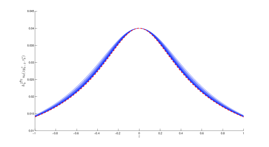
Figure 1: The graph of $v_{k}(z)$ at some selected indexes of $k$, for computing with $\hbar=0.005$ and $a=10$. They converge to the predicted profile (the dash line) as stated in (56) as $k$ increases.

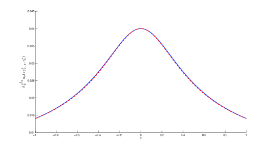
Figure 2: The graph of $v_{k}(z)$ at $k=40$ and the predicted profile given in (56), for computing with $\hbar=0.005$ and $a=0.1$. They coincide within plotting resolution.

In Table 4.3, we give the error in $L^{\infty}$ between $v_{k}(z)$ at index $k=40$ and the predicted profile given in the right hand-side of (56), namely

$$e_{\hbar,a}=\sup_{z\in(-1,1)}\left|v_{40}(z)-M\left(1+(\alpha^{1-p}-1)\lambda^{-2}z^{2}\right)^{-\frac{1}{p-1}}\right|.$$ (67)

These numerical computations give us a confirmation that the computed profiles $v_{k}$ converges to the predicted one. Since the error $e_{\hbar,a}$ tends to $0$ as $\hbar$ goes to zero, the numerical computations also answer to the stability of the blow-up profile stated in $i)$ of Theorem 4. In fact, the stability makes the solution visible in numerical simulations.

$\hbar$	$a=10$	$a=1.0$	$a=0.1$
0.04	0.002906	0.001769	0.002562
0.02	0.000789	0.000671	0.000687
0.01	0.000470	0.000359	0.000380
0.005	0.000238	0.000213	0.000235

Table 4.3: Error in $L^{\infty}$ between the computed and predicted profiles, $e_{\hbar,a}$ defined in (67).

$iii)$ The quality $(h_{k}^{-1}y_{k}^{+})^{2}$ behaves like a linear function.
For making a quantitative comparison between our numerical results and the predicted behavior as stated in $iii)$ of Theorem 11, we plot the graph of $(h_{k}^{-1}y_{k}^{+})^{2}$ against $k$ and denote by $\gamma_{\hbar,a}$ the slope of this curve. Then considering the ratio $\frac{\gamma_{\hbar,a}}{\gamma}$, where $\gamma$ is given in part $iii)$ of Theorem 11. As expected, this ratio $\frac{\gamma_{\hbar,a}}{\gamma}$ would approach one. Figure 3 shows $(h_{k}^{-1}y_{k}^{+})^{2}$ as a function of $k$ for computing with the initial space step $\hbar=0.005$ for different values of $a$. Looking at Figure 3, we see that the two middle curves corresponding the case $a=10$ and $a=1$ behave like the predicted linear function (the top line), while this is not true in the case $a=0.1$ (the bottom curve). In order to make this clearer, let us see Table 4.4 which lists the values of $\frac{\gamma_{\hbar,a}}{\gamma}$ for computing with various values of the initial space step $\hbar$ for three different values of $a$. Here, the value of $\gamma_{\hbar,a}$ is calculated for $20\leq k\leq 40$. As Table 4.4 shows that the numerical values in the case $a=10$ and $a=1$ agree with the prediction stated in $ii)$ of Theorem 11, while the numerical values in the case $a=0.1$ is far from the predicted one.

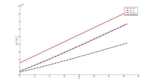
Figure 3: The graph of $(h_{k}^{-1}y_{k}^{+})^{2}$ against $k$, for computing with $\hbar=0.005$ for three different values of $a$.

$\hbar$	$a=10$	$a=1.0$	$a=0.1$
0.04	1.9514	1.9863	1.9538
0.02	1.1541	1.1436	0.8108
0.01	0.9991	1.0052	0.6417
0.005	0.9669	0.9682	0.5986

Table 4.4: The values of $\frac{\gamma_{\hbar,a}}{\gamma}$ for computing with various values of the initial space step $\hbar$ for three different values of $a$.

Appendix A Appendix A

The following lemma from [32] gives the expansion of $\phi(s)$, the unique solution of equation (18) satisfying (19):

Lemma A.1.

Let $\phi$ be a positive solution of the following ordinary differential equation:

$$\phi_{s}=-\frac{\phi}{p-1}+\phi^{p}+\frac{\mu\phi^{p}}{\log^{a}(2+e^{\frac{2s}{p-1}}\phi^{2})}.$$

Assuming in addition $\phi(s)\to\kappa$ as $s\to+\infty$, then $\phi(s)$ takes the following form:

$$\phi(s)=\kappa(1+\eta_{a}(s))^{-\frac{1}{p-1}}\quad\text{as}\quad s\to+\infty,$$

where

$$\eta_{a}(s)\sim C_{*}\int_{s}^{+\infty}\frac{e^{s-\tau}}{\tau^{a}}d\tau=\frac{C_{*}}{s^{a}}\left(1+\sum_{j\geq 1}\frac{b_{j}}{s^{j}}\right),$$

with $C_{*}=\mu\left(\frac{p-1}{2}\right)^{a}$ and $b_{j}=(-1)^{j}\prod_{i=0}^{j-1}(a+i)$.

Proof.

See Lemma A.3 in [32]. ∎

Appendix B Appendix B

We aim at proving the following:

Lemma B.1 (Estimate of $\omega(s)$).

We have

$$|\omega(s)|=\mathcal{O}\left(\frac{1}{s^{a+1}}\right),\quad\text{as}\quad s\to+\infty.$$

Proof.

From Lemma A.1, we write

$$p(\phi(s)^{p-1}-\kappa^{p-1})=-\frac{p\eta_{a}(s)}{p-1}(1+\eta_{a}(s))^{-1}=-\frac{pC_{*}}{(p-1)s^{a}}(1+\eta_{a}(s))^{-1}+\mathcal{O}\left(\frac{1}{s^{a+1}}\right).$$

A direct calculation yields,

$$e^{-s}h^{\prime}\left(e^{\frac{p}{p-1}}\phi(s)\right) =\frac{\mu p\phi^{p-1}(s)}{\log^{a}(2+e^{\frac{2s}{p-1}}\phi^{2}(s))}-\frac{2a\mu e^{\frac{2s}{p-1}}\phi^{p+1}(s)}{(2+e^{\frac{2s}{p-1}}\phi^{2}(s))\log^{a+1}(2+e^{\frac{2s}{p-1}}\phi^{2}(s))}$$

$$=\frac{pC_{*}}{(p-1)s^{a}}(1+\eta_{a}(s))^{-1}+\mathcal{O}\left(\frac{1}{s^{a+1}}\right).$$

Adding the two above estimates, we obtain the desired result. This ends the proof of Lemma B.1. ∎

Lemma B.2 (Estimate of $R(y,s)$).

We have

$$|R(y,s)|=\mathcal{O}\left(\frac{|y|^{2}+1}{s^{a^{\prime}+1}}\right),\quad\text{as}\quad s\to+\infty,$$

with $a^{\prime}=\min\{1,a\}$.

Proof.

Let us write $\varphi(y,s)=\frac{\phi(s)}{\kappa}\nu(y,s)$ where

$$\nu(y,s)=\kappa\left(1+\frac{p-1}{4ps}\sum_{j=1}^{l}y_{j}^{2}\right)^{-\frac{1}{p-1}}+\frac{\kappa l}{2ps}.$$

Then, we write $R(y,s)=\frac{\phi(s)}{\kappa}R_{1}(y,s)+R_{2}(y,s)$ where

$$R_{1}(y,s) =\nu_{s}-\Delta\nu-\frac{y}{2}\cdot\nabla\nu-\frac{\nu}{p-1}+\nu^{p},$$

$$R_{2}(y,s) =-\frac{\phi^{\prime}}{\kappa}\nu-\frac{\phi}{\kappa}\nu^{p}+\phi^{p}\left(\frac{\nu}{\kappa}\right)^{p}+e^{-\frac{ps}{p-1}}h^{\prime}\left(e^{\frac{s}{p-1}}\frac{\phi\nu}{\kappa}\right).$$

The term $R_{1}(y,s)$ is already treated in [34], and it is bounded by

$$|R_{1}(y,s)|\leq\frac{C(|y|^{2}+1)}{s^{2}}+C\mathbf{1}_{\{|y|\geq 2K_{0}\sqrt{s}\}}.$$

To bound $R_{2}$, we use the fact that $\phi$ satisfies (19) to write

$$R_{2}(y,s) =\frac{\nu\phi}{\kappa^{p}}(\kappa^{p-1}-\phi^{p-1})(\kappa^{p-1}-\nu^{p-1})$$

$$+e^{-\frac{ps}{p-1}}\left[h\left(e^{\frac{s}{p-1}}\frac{\phi\nu}{\kappa}\right)-h\left(e^{\frac{s}{p-1}}\phi\right)\right]$$

$$+\left(1-\frac{\nu}{\kappa}\right)e^{-\frac{ps}{p-1}}h\left(e^{\frac{s}{p-1}}\phi\right).$$

Noting that $\nu(y,s)=\kappa+\bar{\nu}(y,s)$ with $|\bar{\nu}(y,s)|\leq\frac{C}{s}(|y|^{2}+1)$, uniformly for $y\in\mathbb{R}$ and $s\geq 1$, and recalling from Lemma A.1 that $\phi(s)=\kappa(1+\eta_{a}(s))^{-\frac{1}{p-1}}$ where $\eta_{a}(s)=\mathcal{O}(s^{-a})$, then using a Taylor expansion, we derive

$$|R_{2}(y,s)|\leq C\left(\frac{|y|^{2}+1}{s^{a+1}}+\mathbf{1}_{\{|y|\geq 2K_{0}\sqrt{s}\}}\right).$$

This concludes the proof of Lemma B.2. ∎

$\begin{array}[]{ll}\textbf{Address:}&\text{Universit\'{e} Paris 13, Institut Galil\'{e}e, LAGA,}\\ &\text{99 Avenue Jean-Baptiste Cl\'{e}ment,}\\ &\text{93430 Villetaneuse, France.}\\ \end{array}$

$\begin{array}[]{ll}\textbf{E-mail:}&\text{vtnguyen@math.univ-paris13.fr}\\ &\text{Hatem.Zaag@univ-paris13.fr}\end{array}$

References

- [1] L. M. Abia, J. C. López-Marcos, and J. Martínez. On the blow-up time convergence of semidiscretizations of reaction-diffusion equations. Appl. Numer. Math., 26(4):399–414, 1998.
- [2] L. M. Abia, J. C. López-Marcos, and J. Martínez. The Euler method in the numerical integration of reaction-diffusion problems with blow-up. Appl. Numer. Math., 38(3):287–313, 2001.
- [3] J. M. Ball. Remarks on blow-up and nonexistence theorems for nonlinear evolution equations. Quart. J. Math. Oxford Ser. (2), 28(112):473–486, 1977.
- [4] G. Baruch, G. Fibich, and N. Gavish. Singular standing-ring solutions of nonlinear partial differential equations. Phys. D, 239(20-22):1968–1983, 2010.
- [5] M. Berger and R. V. Kohn. A rescaling algorithm for the numerical calculation of blowing-up solutions. Comm. Pure Appl. Math., 41(6):841–863, 1988.
- [6] J. Bricmont and A. Kupiainen. Universality in blow-up for nonlinear heat equations. Nonlinearity, 7(2):539–575, 1994.
- [7] A. Cangiani, E. H. Georgoulis, I. Kyza, and S. Metcalfe. Adaptivity and blow-up detection for nonlinear non-stationary convection-diffusion problems. in preparation.
- [8] C. Fermanian Kammerer, F. Merle, and H. Zaag. Stability of the blow-up profile of non-linear heat equations from the dynamical system point of view. Math. Ann., 317(2):347–387, 2000.
- [9] C. Fermanian Kammerer and H. Zaag. Boundedness up to blow-up of the difference between two solutions to a semilinear heat equation. Nonlinearity, 13(4):1189–1216, 2000.
- [10] S. Filippas and R. V. Kohn. Refined asymptotics for the blowup of . Comm. Pure Appl. Math., 45(7):821–869, 1992.
- [11] S. Filippas and W. X. Liu. On the blowup of multidimensional semilinear heat equations. Ann. Inst. H. Poincaré Anal. Non Linéaire, 10(3):313–344, 1993.
- [12] H. Fujita. On the blowing up of solutions of the Cauchy problem for . J. Fac. Sci. Univ. Tokyo Sect. I, 13:109–124 (1966), 1966.
- [13] Y. Giga and R. V. Kohn. Characterizing blowup using similarity variables. Indiana Univ. Math. J., 36(1):1–40, 1987.
- [14] Y. Giga and R. V. Kohn. Nondegeneracy of blowup for semilinear heat equations. Comm. Pure Appl. Math., 42(6):845–884, 1989.
- [15] Y. Giga, S. Matsui, and S. Sasayama. Blow up rate for semilinear heat equations with subcritical nonlinearity. Indiana Univ. Math. J., 53(2):483–514, 2004.
- [16] P. Groisman. Totally discrete explicit and semi-implicit Euler methods for a blow-up problem in several space dimensions. Computing, 76(3-4):325–352, 2006.
- [17] P. Groisman and J. D. Rossi. Asymptotic behaviour for a numerical approximation of a parabolic problem with blowing up solutions. J. Comput. Appl. Math., 135(1):135–155, 2001.
- [18] P. Groisman and J. D. Rossi. Dependence of the blow-up time with respect to parameters and numerical approximations for a parabolic problem. Asymptot. Anal., 37(1):79–91, 2004.
- [19] M. A. Hamza and H. Zaag. Lyapunov functional and blow-up results for a class of perturbations of semilinear wave equations in the critical case. J. Hyperbolic Differ. Equ., 9(2):195–221, 2012.
- [20] M. A. Hamza and H. Zaag. A Lyapunov functional and blow-up results for a class of perturbed semilinear wave equations. Nonlinearity, 25(9):2759–2773, 2012.
- [21] M. A. Herrero and J. J. L. Velázquez. Blow-up profiles in one-dimensional, semilinear parabolic problems. Comm. Partial Differential Equations, 17(1-2):205–219, 1992.
- [22] M. A. Herrero and J. J. L. Velázquez. Flat blow-up in one-dimensional semilinear heat equations. Differential Integral Equations, 5(5):973–997, 1992.
- [23] M. A. Herrero and J. J. L. Velázquez. Generic behaviour of one-dimensional blow up patterns. Ann. Scuola Norm. Sup. Pisa Cl. Sci. (4), 19(3):381–450, 1992.
- [24] M. A. Herrero and J. J. L. Velázquez. Blow-up behaviour of one-dimensional semilinear parabolic equations. Ann. Inst. H. Poincaré Anal. Non Linéaire, 10(2):131–189, 1993.
- [25] M. A. Herrero and Juan J. L. Velázquez. Comportement générique au voisinage d’un point d’explosion pour des solutions d’équations paraboliques unidimensionnelles. C. R. Acad. Sci. Paris Sér. I Math., 314(3):201–203, 1992.
- [26] I. Kyza and C. Makridakis. Analysis for time discrete approximations of blow-up solutions of semilinear parabolic equations. SIAM J. Numer. Anal., 49(1):405–426, 2011.
- [27] H. A. Levine. Some nonexistence and instability theorems for solutions of formally parabolic equations of the form . Arch. Rational Mech. Anal., 51:371–386, 1973.
- [28] N. Masmoudi and H. Zaag. Blow-up profile for the complex Ginzburg-Landau equation. J. Funct. Anal., 255(7):1613–1666, 2008.
- [29] F. Merle and H. Zaag. Stability of the blow-up profile for equations of the type . Duke Math. J., 86(1):143–195, 1997.
- [30] F. K. N’gohisse and T. K. Boni. Numerical blow-up for a nonlinear heat equation. Acta Math. Sin. (Engl. Ser.), 27(5):845–862, 2011.
- [31] V. T. Nguyen. Numerical analysis of the rescaling method for parabolic problems with blow-up in finite time. submitted, 2014.
- [32] V. T. Nguyen. On the blow-up results for a class of strongly perturbed semilinear heat equation. submitted, 2014.
- [33] V. T. Nguyen and H. Zaag. Contruction of a stable blow-up solution for a class of strongly perturbed semilinear heat equation. submitted, 2014.
- [34] J. J. L. Velázquez. Higher-dimensional blow up for semilinear parabolic equations. Comm. Partial Differential Equations, 17(9-10):1567–1596, 1992.
- [35] J. J. L. Velázquez. Classification of singularities for blowing up solutions in higher dimensions. Trans. Amer. Math. Soc., 338(1):441–464, 1993.
- [36] F. B. Weissler. Existence and nonexistence of global solutions for a semilinear heat equation. Israel J. Math., 38(1-2):29–40, 1981.