BEAM–BEAM EFFECTS IN BEPCII

Abstract

We first introduce the design parameters of the Beijing Electron–Positron Collider II (BEPCII) and the simulation study of beam–beam effects during the design process of the machine. The main advances since 2007 are briefly introduced and reviewed. The longitudinal feedback system was installed to suppress the coupled bunch instability in January 2010. The horizontal tune decreased from 6.53 to 6.508 during the course of data taken in December, 2010. The saturation of the beam–beam parameter was found in 2011, and the vacuum chambers and magnets near the north crossing point were moved 15 cm in order to mitigate the long range beam–beam interaction. At the beginning of 2013, the beam–beam parameter achieved 0.04 with the new lower $\alpha_{p}$ lattice and the peak luminosity achieved $7\times 10^{32}\text{~{}cm}^{-2}\text{~{}s}^{-1}$.

1 Introduction

The Beijing Electron–Positron Collider (BEPC) was constructed for both high energy physics and Synchrotron Radiation (SR) research. As a unique $e^{+}e^{-}$ collider operating in the $\tau$-charm region and the first SR source in China, the machine has been operated for well over 16 years since it was put into operation in 1989.

BEPCII is an upgrade project from BEPC. It is a double ring machine. Following the success of KEKB, the crossing scheme was adopted in BEPCII, where two beams collide with a horizontal crossing angle of $2\times 11$ mrad. The design luminosity of BEPCII is $1.0\times 10^{33}\mbox{~{}cm}^{-2}\mbox{~{}s}^{-1}$ at $1.89~{}$GeV, which is about $100$ times higher than BEPC [1]. The main design collision parameters are shown in Table 1.

Table 1: Design Parameters of BEPCII.

E	1.89 GeV	$\nu_{s}$	0.034
$I$	910 mA	$\alpha_{p}$	0.024
$I_{b}$	9.8 mA	$\sigma_{z0}$	0.0135 m
$n_{b}$	93	$\sigma_{z}$	0.015 m
$V_{rf}$	1.5 MV	$\epsilon_{x}$	144 nmrad
$\beta_{x}^{*}/\beta_{y}^{*}$	1.0/0.015 m	Coupling	1.5%
$\nu_{x}/\nu_{y}$	6.53/5.58	$\xi_{y}$	0.04
$\theta_{c}$	22 mrad	$\tau_{x}/\tau_{y}/\tau_{z}$	3.0e4/3.0e4/1.5e4

In March 2013, the peak luminosity achieved $7.0\times 10^{32}\text{~{}cm}^{-2}\text{~{}s}^{-1}$ with 120 bunches and beam current 730 mA, where a lower $\alpha_{p}$ lattice was used.

In the following, we first introduce the simulation study of the beam–beam interaction during the design course of the machine. Then we review the performance and optimization of the real machine.

2 Simulation Study During Design

2.1 Code Development

We have developed new parallel strong–strong beam–beam code, which is used to study the effects in BEPCII [2]. The main characteristics of the code are listed below.

• Particle-in-cell. The Triangular Shaped Cloud (TSC) method is employed for the charge assignment, where the charge of each macroparticle is assigned to its nine nearest points by weight.

• Synchrotron motion is included. The transportation through the arc is same as that of Hirata’s BBC code [3].

• The beam–beam potential is calculated by solving the Poisson equation with open boundary.

• Bunch length effect is included by longitudinal slices and the interpolation of beam–beam potential is done when the collision between two slices is considered, which helps to reduce the required slice number.

• It is assumed that a particle in one slice will not jump into non-adjacent ones on the next turn. It seems that this assumption has been valid so far, especially in the ordinary collision scheme (where the required slice number is only about 5).

• Lorentz boost is used to consider the crossing angle effect [4].

2.2 Code Check

• The geometrical factor of luminosity reduction for head-on collision. The loss in luminosity due to geometrical effect for nominal BEPCII parameters is 86%, and the code tracking result agrees well.

• The geometrical factor of luminosity reduction for collision with finite crossing angle. The loss in luminosity due to geometrical effect for design BEPCII parameters is 80%, and the code tracking result agrees well.

• The beam–beam field calculated by the code for the Gaussian beam distribution agrees well with the Bassetti–Erskine formula.

• The synchro-betatron mode agrees well with that predicted by the hollow beam matrix model [5].

• The luminosity result for BEPCII agrees well with that of K. Ohmi’s code [6].

2.3 Simulation Result

The achieved beam–beam parameter $\xi$ with collision is defined as

$$\xi_{u}=\frac{Nr_{e}}{2\pi\gamma}\frac{\beta_{u}^{0}}{\sigma_{u}(\sigma_{x}+\sigma_{y})}$$ (1)

where $\beta^{0}$ is the nominal beta function without collision, and $\sigma$ is the disturbed beam size with collision. If we don’t consider the finite bunch length and finite crossing angle, the bunch luminosity can be represented as

$$L=\frac{N^{2}f_{0}}{4\pi\sigma_{x}\sigma_{y}}$$ (2)

where $\sigma$ is the disturbed beam size with collision. In the normal case, $\sigma_{y}\ll\sigma_{x}$, the achieved $\xi_{y}$ can be represented by luminosity,

$$\xi_{y}=\frac{2r_{e}\beta_{y}^{0}}{N\gamma}\frac{L}{f_{0}}.$$ (3)

With the design parameters, the maximum $\xi_{y}$ only achieves 0.025, which is shown in Fig. 1. This is bad news for the BEPCII team, since $\xi_{y}$ needs to achieve 0.04 if we want to achieve the designed luminosity with the designed beam current. We therefore did some estimation to determine if it would be feasible to inject more bunches, and it seems that this would be possible.

Figure 1: The achieved $\xi_{y}$ and bunch luminosity versus bunch current with design parameters.

The beam–beam performance is very sensitive to the working point. The normalized luminosity versus tune is depicted in Fig. 2. The best working point is near (0.505,0.570), where the luminosity is about 80% of the design value. That is to say, we could achieve $8\times 10^{32}\text{~{}cm}^{-2}\text{~{}s}^{-1}$ with the designed bunch current, bunch number and optimized working point.

Figure 2: Tune survey of luminosity. The luminosity is normalized to the design value.

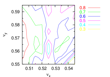
The full horizontal crossing angle between colliding beams is 22 mrad. The luminosity reduction factor is less than 10% at (0.53,0.58), however it is about 30% at (0.51,0.57). It seems that the luminosity loss due to a finite crossing angle is more serious the closer the horizontal tune is to $0.5$, the high luminosity working point region.

We also tried to analyze the coupling contribution and carried out some simulations at different working points. The results are summarized in Table 2. It seems that we have to move the horizontal tune closer to $0.5$ and ensure that the emittance coupling is less than 0.5% if $\xi_{y}$ is expected to achieve 0.04.

Table 2: Coupling contribution at different working point.

Tune	Coupling	Max $\xi_{y}$	Lum
(0.510, 0.575)	0.5%	0.041@11 mA	12.3e30
	1.0%	0.037@12 mA	12.1e30
	1.5%	0.034@13 mA	12.1e30
(0.530, 0.580)	0.5%	0.026@7 mA	5.0e30
	1.5%	0.026@13 mA	9.2e30
(0.535, 0.575)	0.5%	0.031@9 mA	7.6e30
	1.0%	0.027@9 mA	6.6e30
	1.5%	0.023@9 mA	5.6e30
(0.540, 0.590)	0.5%	0.025@11 mA	7.6e30
	1.0%	0.024@11 mA	7.2e30

3 Performance and Optimization

The first electron beam was stored in the SR ring in November 2006. Optics measurement and correction was studied at that time. The backup collision mode was first tuned in the spring of 2007, during the course of which we learned the collision tuning. The superconducting final focus magnet was installed in the summer of 2007. The detector was installed in June 2008, and this completed the construction of the machine. Here, we review the machine tuning history in chronological order.

3.1 Phase I: Autumn of 2008 to Summer of 2010

The big events in this period are listed below.

• January 2009. Profile monitor, which caused very strong longitudinal multibunch instability, was removed from the positron ring.

• May 2009. Horizontal tune was moved to $0.51$ from $0.53$. Luminosity reached $3\times 10^{32}\text{~{}cm}^{-2}\text{~{}s}^{-1}$, which is the ‘design goal’ of the government funding agency.

• January 2010. Longitudinal feedback system was installed and began to work.

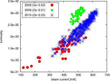
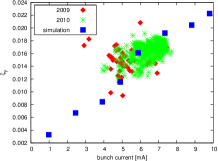
Figure 3 shows the luminosity versus beam current and Fig. 4 shows the beam–beam parameter versus bunch current. The longitudinal coupled bunch instability still reduced the luminosity performance even after the removal of the profile monitor, which caused very strong instability, from the positron ring. In order to increase the luminosity with the same beam current, we tried to move the horizontal tune closer to $0.5$ in May 2009. The peak luminosity increased from 2 to $3\times 10^{32}\text{~{}cm}^{-2}\text{~{}s}^{-1}$. Since the detector background is too high to take data with $Q_{x}\sim 0.51$, the machine continued to run with $Q_{x}\sim 0.53$ in the following normal data collection run. In the first half of 2010, the longitudinal feedback system began to work and the peak luminosity achieved $3\times 10^{32}\text{~{}cm}^{-2}\text{~{}s}^{-1}$ with $Q_{x}\sim 0.53$. The maximum $\xi_{y}$ is about 0.02 when $Q_{x}\sim 0.53$, which is less than the simulated 30% percent (see Table 2).

Figure 3: Luminosity versus beam current in 2009 and 2010. The difference between the red (2009) and blue (2010) dots comes from the suppression of longitudinal multibunch instability.

Figure 4: Beam–beam parameter versus bunch current. The left figure shows that $Q_{x}\sim 0.53$ and the right shows that $Q_{x}\sim 0.51$. The longitudinal feedback system begins to work in 2010.

3.2 Phase II: Autumn of 2010 to Summer of 2011

The big events in this period are listed below.

• July 2010. It was found that the final focus magnet and vacuum chamber on one side of the detector was displaced by about 10 mm in the horizontal direction. It was aligned in the summer shutdown.

• December 2010. Detector background was reduced with $Q_{x}\sim 0.51$. The physics people could take data near the 0.51 working point.

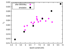
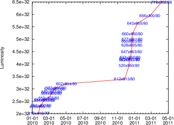
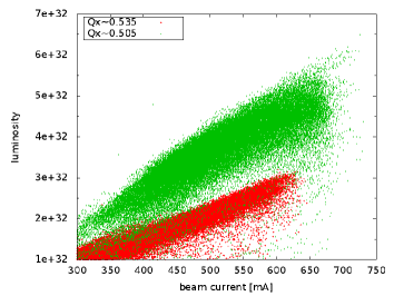
The most important advance in this period is the reduction of the detector background with $Q_{x}\sim 0.51$, since the physics people could take data at the working point and the accelerator people had enough time to do the luminosity tuning. The detector background is mainly optimized by the closed orbit tuning along the ring. Figure 5 shows the peak luminosity record from the beginning of 2010 to the summer of 2011. It was very exciting near the start of 2011 since a new record would be born only in a few days. The peak luminosity was $6.5\times 10^{32}\text{~{}cm}^{-2}\text{~{}s}^{-1}$ in 2011. The comparison of luminosity at different working points is shown in Fig. 6, which very obviously shows that a working point closer to $0.5$ means a higher luminosity.

Figure 5: Peak luminosity record from the beginning of 2010 to the summer of 2011. The colliding beam current and bunch number is also shown in the figure.

Figure 6: Luminosity performance at different working points.

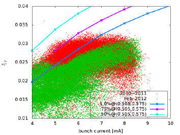
The 2010–2011 commissioning year was very successful and exciting, but there was some confusion when we saw the beam–beam performance. The achieved $\xi_{y}$ is shown in Fig. 7. There exist clear saturation phenomenon for $\xi_{y}$ and the maximum is about 0.033. We should explain what caused the saturation.

Figure 7: Achieved beam–beam parameter in 2010–2011. The lines shows the simulation result with different coupling.

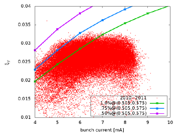
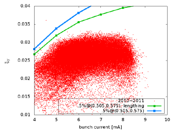
Figure 8 shows the bunch lengthening effect. It seems this effect does not bring very much luminosity loss, and the maximum beam–beam parameter is still above 0.04.

Figure 8: Beam–beam loss due to bunch lengthening, which does not explain the beam–beam parameter saturation in real machine.

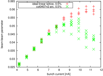
The nonlinear arc may also reduce the luminosity performance. We use Hirata’s BBC [3] code as a pass method in Accelerator Toolbox (AT) [7] to simulate the weak–strong beam–beam interaction. The map in the arc is implemented using the element-by-element symplectic tracking in AT. Figure 9 shows the comparison between the ideal transfer matrix map and element-by-element tracking in arc. The lattice really reduces the beam–beam performance, but we did not believe that the saturation was mainly caused by the crosstalk between nonlinear arc and beam–beam force. On the other hand, we could not ignore the simulation result, which told us that we should put more emphasis on the sexupole optimization.

Figure 9: The luminosity loss due to the realistic arc. The arc map is implemented using element-by-element tracking. The ideal linear lattice means the map is represented by a transfer matrix.

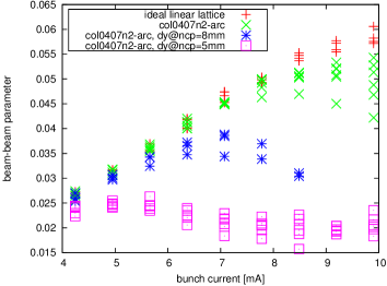
There is another crossing point (NCP) in the north of the two rings, where the colliding beams are separated vertically by about 8 mm and the full horizontal angle is about $2\times 0.15$ rad (17.7^∘). We still use the weak–strong code (AT and BBC) to study the parasitic beam–beam effect, which is shown in Fig. 10. The achieved $\xi_{y}$ is only about 0.035 with 8 mm separation at NCP

Figure 10: The luminosity loss due to nonlinear arc and long range beam–beam interaction at NCP.

3.3 Phase III: Autumn of 2011 to Summer of 2012

The big events in this period are listed below.

• In the summer shutdown of 2011, the NCP chambers and magnets were moved 15 cm, 1/4 of the rf bucket. The horizontal separation between colliding bunches is greater than $30\sigma_{x}$.

After the hardware modification, the beam–beam performance did not increase as expected, which is shown in Fig. 11. This could be explained to some extent by the large longitudinal offset of the collision point. In 2011–2012 commissioning year, the offset is about 3 mm, and it is about 6 mm in February 2012. We did not put enough emphasis on monitoring the parameter during collision at that time.

Figure 11: Beam–beam parameter achieved in 2011 and 2012. The mitigation of long range beam–beam interaction at NCP did not bring any improvements.

3.4 Phase IV: Autumn of 2012 to March 2013

The big events in this period are listed below.

• Lower $\alpha_{p}$ mode was first tested at 2.18 GeV in February 2013. The $\xi_{y}$ record 0.033 was broken after about two years.

• One bunch every three buckets, and even one bunch every two buckets, injection was tested in the machine study of March 2013. The peak luminosity achieved $7.0\times 10^{32}\text{~{}cm}^{-2}\text{~{}s}^{-1}$ at 1.89 GeV.

The momentum compaction factor of the new lattice is about 0.017, and the old one is 0.024. The reduction of $\alpha_{p}$ is achieved by increasing the horizontal tune from 6.5 to 7.5. During the lattice design, we also optimized the chromatic distortion and some nonlinear resonance driving terms. However we still did not establish a so-called ‘standard’ that could tell us if the lattice is good enough.

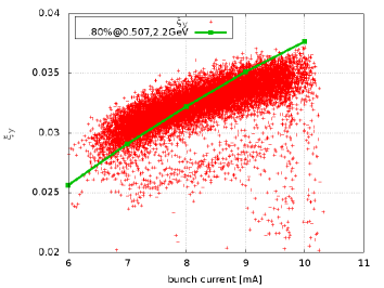
The achieved beam–beam performance at 2.18 GeV is shown in Fig. 12. We also did some machine study in order to increase the peak luminosity at 1.89 GeV. The achieved beam–beam parameter with different bunch pattern is shown in Fig. 13. The maximum $\xi_{y}$ is above 0.04. It seems that the multibunch effect reduces the beam–beam performance, which would be a serious limitation if we were to continue to increase the luminosity.

Figure 12: Achieved beam–beam parameter at 2.18 GeV with new lattice in 2013.

Figure 13: Achieved beam–beam parameter at 1.89 GeV with different bunch pattern in 2013.

4 Summary

We review the collision optimization history of BEPCII. The suppression of multibunch longitudinal instability and moving the horizontal tune close to $0.5$ helped us to increase the luminosity. The mitigation of long range beam–beam interaction seems not so effective as expected, indicating that maybe the real vertical separation is greater than estimated. The lower $\alpha_{p}$ lattice helped us to achieve the $\xi_{y}$ record of 0.04 at 1.89 GeV.

The simulation study is very important both in the design and the daily commissioning. It gives a benchmark in normal operation and lets us know if the status is optimized enough, even though we could approach the simulation result and never go beyond it. The difference between the simulation and the optimized result is about 10–20%. It should also be emphasized that we would like to use the maximum achieved $\xi_{y}$ in the simulation as the beam–beam limit in the simulation.

Increasing beam current is a must to increasing the luminosity. However, it seems the multibunch effect is very serious. The study to cure the instability and even find the instability source will be very important in the future. In the near future, we’ll test a new lattice with $alpha_{p}$ about 0.017, larger emittance (100 nm$\rightarrow$130 nm) and lower $\beta_{y}$ (1.5 cm$\rightarrow$1.35 cm). The colliding bunch current could be higher with the new mode and the beam current could be higher with same bunch number. It is expected that this could help us to increase the luminosity.

References

- [1] Design Report of BEPCII–Accelerator Part (2nd ed) (2003).
- [2] Y. Zhang, K. Ohmi and L. Chen, Phys. Rev. ST Accel. Beams 8 (2005) 074402.
- [3] BBC: Program for Beam–Beam Interaction with Crossing Angle. http://wwwslap.cern.ch/collective/hirata/
- [4] K. Hirata, Phys. Rev. Lett. 74 (1995) 2228-2231.
- [5] E.G. Stern, J.F. Amundson, P.G. Spentzouris, and A.A. Valishev, Phys. Rev. ST Accel. Beams 13 (2010) 024401.
- [6] K. Ohmi, Phys. Rev. E 62 (2000) 7287.
- [7] A.Terebilo, SLAC-PUB-8732 (2001).