Global analysis of the experimental data on meson hadroproduction
Abstract
We carry out a global analysis of the experimental data on the production cross section and the ratio at the LHC and the Tevatron. The related long-distance matrix elements (LDMEs) at both leading order (LO) and next-to-leading order (NLO) in the QCD coupling constant are renewed. We also present the transverse momentum distribution of the production cross section and the ratio for several experimental conditions and find that NLO predictions agree with all sets of experimental data. By contrast, at LO, one cannot explain all the data with a unique value of the color-octet LDME. A brief analysis of the nonrelativistic QCD scale dependence of the cross sections shows that, for the conditions we are concerned with in this paper, the dependence can be almost totally absorbed into the LDME.
pacs:
12.38.Bx, 12.39.St, 13.85.Ni, 14.40.PqI introduction
Since the Large Hadron Collider (LHC) started its run, many experimental results have come out that have provided an opportunity to carry out further investigation of the phenomenology of QCD-based effective theories. Nonrelativistic QCD (NRQCD) is one of the most successful effective theories describing quarkonium production and decays Bodwin et al. (1995). Under the NRQCD framework, the cross section is factorized into the summation of the products of the short-distance coefficient (SDC), which is independent of the quarkonium state and can be calculated perturbatively, and the long-distance matrix element (LDME), which only depends on the quarkonium state and requires the fit of experimental data to extract its value. The cross section for the process of heavy quarkonium production or decay can be expressed as
| (1) |
where is the SDC for the state , and is the LDME of state for quarkonium .
NRQCD succeeded in many processes where the color-singlet (CS) model Einhorn and Ellis (1975); Ellis et al. (1976); Chang (1980); Berger and Jones (1981); Baier and Ruckl (1982) failed; however, it still faces many challenges. polarization at hadron colliders is among the most puzzling questions that NRQCD encounters. References Butenschoen and Kniehl (2012); Chao et al. (2012) investigated the polarization of directly produced , while Ref. Gong et al. (2013) provided polarization results for prompt hadroproduction, which is the first next-to-leading-order (NLO) result comparable with experiment. The three letters employed three sets of LDMEs, which were obtained from different fit strategies. All of them can describe production, yet none of them can explain all the polarization measurements. In addition, the universality of the LDMEs is another challenge. Reference Butenschoen and Kniehl (2011) reconciled experimental data of production at the Tevatron and HERA;however, their LDMEs resulted in unphysical cross sections when employed to associated with a photon production at hadron colliders Li and Wang (2014). Another interesting example is the transverse momentum () integrated cross sections for the hadroproduction. The theoretical results at QCD NLO obtained with collinear factorization Maltoni et al., (2006); Feng et al. (2015) overshoot the experimental data. Having resummed (where denotes the Bjorken-) and considered the all-twist contributions in the dense side, Ma and Venugopalan Ma and Venugopalan (2014) remedied the discrepancy. However, they Ma and Venugopalan (2014) did not include the and feeddown contributions. Whether the inclusion of these parts will ruin the conclusions requires further investigation. Actually, Ref. Hagler et al. (2001) has already studied the production processes in which the of the completely comes from the initial states. Exploiting the unintegrated gluon distribution, the authors announced that the color-octet (CO) LDME for is almost an order of magnitude smaller than the one obtained through the collinear factorization calculations. Reference Shuvaev et al. (2015), however, found that the final-state gluon emission processes actually dominate the hadroproduction in the midrapidity region. For the above reasons, testing NRQCD is still an important work.
P-wave quarkonia productions provide an excellent laboratory to test NRQCD. Above all, at LO in (the typical relative velocity of quark and antiquark in quarkonium), only one LDME is to be obtained from experiment; one does not suffer from the entanglement of too many free parameters in the fit of experimental data, in contrast to the case Butenschoen and Kniehl (2011, 2012); Ma et al. (2011a, b); Chao et al. (2012); Gong et al. (2013). Further, at NLO, the distribution of both and channels behaves as in the large region. Higher order corrections cannot exceed this behavior; thus, one can expect NLO predictions to give a good precision in this phase space region. In contrast to the case, the significance of NNLO correction is still in the mist. Finally, feeddown from higher excited states to P-wave quarkonia, say, , , , or , can almost be neglected [e.g., at LHCb Aaij et al. (2012a, b, 2011)]. Notice the advantages stated above:we say the case of is “clean”; it is much easier to make definite conclusions in this case than in the case.
On the other hand, the study of production is not only important itself for phenomenological concerns, but also provides an opportunity for precise study of phenomenology (e.g.,Ref. Gong et al. (2013) indicates that feeddown contribution is essential to the study of polarization). Many theoretical works on production have been published. The authors of Refs. Cho and Leibovich (1996a, b); Braaten et al. (2000); Sharma and Vitev (2013) obtained LDME for production at LO and employed them to the prediction of prompt hadroproduction and/or polarization. Ma et al. Ma et al. (2011c) presented the first NLO study of hadroproduction and gave a favorable choice of the LDME for production. Li et al. Li et al. (2011) calculated production associated with a pair at hadron colliders. Shao et al. Shao and Chao (2014); Shao et al. (2014) provided a detailed study on the polarization of hadroproduced and -generated ; at the same time, they compared the theoretical prediction with some of the recent experimental data Abulencia et al. (2007); Aaij et al. (2012c); Chatrchyan et al. (2012). Likhoded et al. Likhoded et al. (2014) calculated hadroproduction at LO in and extracted both the CS and CO LDMEs from the fit of the experimental data, where their CS LDME is several times larger than the value obtained by the potential model and higher order terms in contribute significantly.
This paper is devoted to the theoretical predictions of hadroproduction, for one thing, as an alternative test of NRQCD. Recently, a number of experiment results have come out from the LHC collaborations, among which are many measurements on the yield and the ratio . This paper will answer the question whether a single LDME can explain all the experimental data. For another thing, the popular values of the LDMEs for production, both at LO and NLO, were all given before these experimental results were published; they are out of date. This paper will provide a detailed analysis on the determination of the LDMEs and reasonable values of it at both LO and NLO. Finally, as suggested in Ref. Wang and Zhang (2015), we also observe the NRQCD scale dependence of the cross sections to determine whether NLO prediction stands up.
This paper is organized as follows. Section II gives a brief introduction to the NRQCD framework for hadroproduction calculation. In Sec. III, we present the parameter choices in our numerical computation and an analysis to see whether the NRQCD scale dependence is severe. In Sec. IV, we present the results of the fit and the values of the LDMEs at both LO and NLO and investigate the universality of the LDMEs in detail. Section VI is a concluding remark.
II production in NRQCD framework
This section provides quite a brief review of the NRQCD formulas for the calculation of production. We do not discuss in detail how the equations are derived. Interested readers can refer to some relative references, e.g. Petrelli et al. (1998); Wang and Zhang (2015).
For production at LO in , Eq.(1) can be written as
| (2) |
. The value of CS LDME can be evaluated through Bodwin et al. (1995)
| (3) |
, where is the derivative of the wave function of the related quarkonium with respect to the radius at the origin.
The calculation of has been described in detail in many of our previous papers;see,e.g., Gong et al. (2011). To evaluate , we notice that it is independent of the long-distance asymptotic states and replace in Eq.(2) with a state , so that we obtain
| (4) |
, where we have used the relation . We should keep in mind that Eq.(4) is to extract CS SDC, which is expanded in . As a result, the quantities and should also be evaluated perturbatively, and the value of in them should be in accordance with that in the SDCs. The left- and right-hand side of Eq.(4) should keep those terms up to the same order as in the perturbative expansion. The evaluation of follows the ordinary procedure: writing the squared amplitudes through reading Feynman diagrams and multiplying it by the flux density and the phase space unit. Both and are infrared (IR) divergent, and the IR divergences from the two quantities cancel each other.
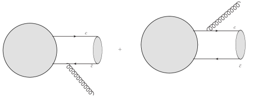
We adopt the two-cutoff phase space slicing method Harris and Owens (2002) and find that the cross section excluding the terms (denoted as ) corresponding to the squared real-correction diagrams, in which a gluon connects the quarkonium (as displayed in Fig. 1), integrated over the gluon soft region is free of divergence. We denote this finite part of the cross section as . Neglecting the finite terms proportional to the size of the small region, can be expressed as
| (5) |
where is 3 for SU(3) gauge field and
| (6) |
with and being the energy and absolute value of momentum of , respectively, the Euler’s constant, and the scale to complement the dimension. is an arbitrary positive number small enough to provide the soft approximation with sufficient accuracy.
Up to the order maintained in our calculation, the transition rate of state into can be calculated in the dimensional regularization scheme as
| (7) |
where is defined as
| (8) |
and
| (9) |
in the -cutoff (in which is the upper bound of the integrated gluon energy) and renormalization scheme, respectively. is a scale rising from the renormalization of the LDME.
Substituting Eqs.(7) and (5) into Eq.(4), we can solve the SDC for as
| (10) |
where
| (11) |
the expressions of which for the -cutoff and renormalization scheme are
| (12) |
and
| (13) |
respectively.
Both of the terms on the right-hand side of Eq.(10) are finite. Now, all the short-distance coefficients are IR divergence free;then the components for calculating the cross section for hadroproduction are well defined.
III numerical calculation and the analysis on dependence
To calculate and , we apply our Feynman diagram calculation package (FDC) Wang (2004) to generate the entire needed FORTRAN source.
Before we present the numerical results, we should comment on the obtaining the CO LDME. Focusing on the last two terms in the right-hand side of Eq.(14), one can notice that, if varies its value, in order to fit the cross section to the experimental data, the LDME in the last term should change accordingly, which is to say, the dependence on is partly absorbed into the CO LDME. If we proceed with our calculation to infinite order in , the dependence can be totally absorbed into the CO LDME. Consequently, this scale actually can be any positive value holding the convergence of expansion. If our results significantly depend on , the dropped terms in higher orders must contribute significantly, and the calculation up to this order does not reach a sufficient accuracy. Up to NLO, the condition of independence requires
| (15) |
as well as that the proportional ratio should be universal for all the processes. We define a quantity
| (16) |
to determine whether the dependence is severe. If is constrained in a small range throughout the whole region for all the processes, we know for sure the dependence on can be absorbed into the LDME and vice versa. In this paper, we provide the values of the CO LDME for different renormalization schemes and choices.
In the numerical calculation, we have the following common choices of parameters: Eichten and Quigg (1995) for both LO and NLO calculation, and . The soft cutoff independence is checked in the calculation and is used. Since the energy scale of most of the phase space region exceeds b-quark mass, is used. We employ CTEQ6M Pumplin et al. (2002) as the parton distribution function (PDF) and two-loop running for up-to-NLO calculation, and CTEQ6L1 Pumplin et al. (2002) and one-loop running for LO. The renormalization and factorization scales are chosen as .
In our fit, we exclude the data points. This is because, for one thing, relativistic correction contributes a part proportional to the QCD LO SDC, when is larger than about 7GeV Xu et al. (2012); this part can be complemented by modifying the values of the LDMEs, while below 7GeV, this is not true. For another thing, the terms might ruin the perturbative expansion in this region Kang et al. (2014); Ma and Venugopalan (2014).
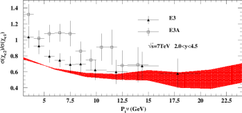
To extract the CO LDME, we employ all the existing data on hadroproduction except for those in Ref. Abe et al. (1997a), which measured the fraction of the hadroproduction cross section through the feeddown to the prompt one. Reference Abe et al. (1997b) provided the prompt hadroproduction cross section with the same center-of-mass energy and rapidity range. However, the ’s of the two sets of data do not coincide.Thus, we cannot extract the exact central values and error bars of the hadroproduction cross sections and consequently we cannot use these data directly. For this reason, we give up using them in our fit. There are six sets of data involved in our analysis. All of them are listed in Table 1. Except for the data mentioned above, we also noticed another set of data (denoted as E3A), which was published in Ref. Aaij et al. (2012c). Since the data in E3 are the updated version of those in E3A, we do not use E3A for fit;however, we plot them in the figures for reference.
| Abbreviation | E1 | E2 | E3 | E4 | E5 | E6 |
| Center-of-mass energy(TeV) | 1.96 | 7 | 7 | 7 | 7 | 7 |
| Rapidity range | ||||||
| Collaboration | CDF Abulencia et al. (2007) | LHCb Aaij et al. (2012b) | LHCb Aaij et al. (2013) | CMS Chatrchyan et al. (2012) | ATLAS Aad et al. (2014) | ATLAS Aad et al. (2014) |
| Content | cross section | cross section | cross section |
In Refs. Abulencia et al. (2007); Aaij et al. (2012b, 2013); Chatrchyan et al. (2012) (corresponding to E1E4), the values of are given for the generated from feeddown, in accordance with which we should do the so-called shift as . Here we choose Olive et al. (2014) , , ,and , which are different from Ref. Gong et al. (2013), where and are and , respectively. The branching ratios Olive et al. (2014) are , , and for to , respectively.
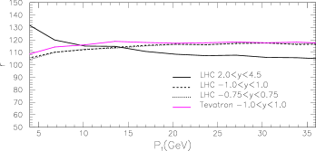
Before we carry out the fit, we shall first investigate whether defined in Eq.(16) is universally a constant to hold the independence. E2 and E3 are in the same experimental condition, as are E5 and E6; accordingly, there are four conditions to present. For these experimental conditions, the values of are presented in Fig.2. We can see that, except for E2 (as well as E3), for all three conditions, is almost a constant, ranging from about 104 to 118, as varies from to . As we expected in the introductory section that NLO results should provide a sufficiently precise prediction, the dependence cannot be severe. For E2, the situation is a little worse ( ranges from 132 to 105), yet, not so bad to ruin the results. We can now expect that, for E1 and E4E6, the theoretical prediction should be in good agreement with the experiment, and if we carry out the fit by employing the four sets of data individually, we should obtain almost the same results of the values of the LDME. For E2 and E3, the theoretical prediction might agree with the experiment qualitatively.
is not always a constant up to NLO precision. As an example, for hadroproduction, varies significantly for different experimental conditions and phase space regions. Interested readers can refer to Ref. Wang and Zhang (2015), in which the detailed results for hadroproduction are presented.
IV Numerical results and comparison to the experimental data
We present the values of the CO LDME extracted from the fit of each set of the experimental data at both LO and NLO, and see if they correspond with one another. In the rest of this paper, we abbreviate as .
For LO calculation,
| (17) | |||
and the are 6.4, 0.0078, 1.1, 0.69, 0.11, and 0.43, respectively.
For NLO calculation, as in -cutoff renormalization scheme,
| (18) | |||
and the are 2.8, 0.034, 0.18, 0.17, 0.068, and 0.35, respectively.
To begin with, we can see that, for all the conditions except for E2, the for NLO is smaller than that for LO. Moreover, for E1 and E4E6, the obtained values of the CO LDME for NLO are almost the same ( ranges from 1.97 to 2.04). As we analyzed in the previous section, we do not expect theoretical prediction for E2 and E3 to agree with the experiment in high precision; however, even for E2 and E3, the obtained values of the CO LDME are very close to those for E1 and E4E6. By contrast,for the values of obtained for the LO range from 0.13 to 1.26, the largest is about ten times the smallest, and there is no common value for any group of the sets of data; the distribution of the values is dispersive. We can conclude that, no universal value exists for LO LDME, since up to LO, the precision is not sufficient to describe all the experiments. We can also see that the LDME given in Ref. Cho and Leibovich (1996b) is too large. One might make wrong conclusions if using that value. The LDME given in Ref. Sharma and Vitev (2013) is much larger than the upper bound of the series of the values presented above. The large value of the LDME might lead to overestimation of the absorption effect (as well as other nuclear matter effects).
Now we carry out a global fit, using all the experimental data in E1E6 for LO, and E1 and E4E6 for NLO, and obtain
| (19) |
The are 2.4 and 0.47 for LO and NLO, respectively. The consideration is that we trust the precision of the NLO results for E1 and E4E6. However, for E2 and E3, the situation is not clear. Thus, we fit E1 and E4E6 to obtain NLO CO LDME as a default value to present our results, and we employ the LDME to see whether it can explain the experiment E2 and E3.
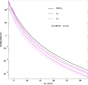
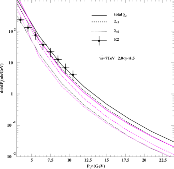

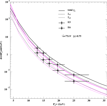


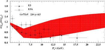
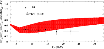
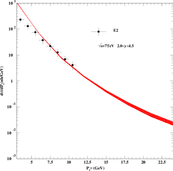
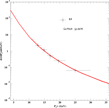
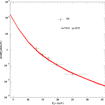
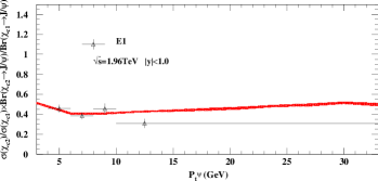
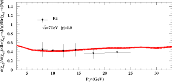
Theoretical predictions for the production cross section and the ratio are listed in Figs.3 and 4 , respectively. References Abulencia et al. (2007); Aaij et al. (2012b, 2013); Chatrchyan et al. (2012) only provide results for , while Ref. Aad et al. (2014) provides results for both and . Since our calculations are carried out at , for this reason, the distributions for E5 and E6 illustrated in Fig.3 are with respect to . Since the uncertainty of the LDME at NLO is small, we do not draw the band rising from this uncertainty. However, the uncertainty of the LDME for LO is quite large, but we do not bother with this matter here. We will provide a more reasonable band for LO uncertainty later.
We can see from Figs.3 and 4 that NLO results are in very good agreement with all the experiments, while LO results cannot agree with most of the experimental data. As we mentioned above, for E2 and E3, the NLO calculation might not be able to provide sufficiently precise results, since as displayed in Fig.2 that dependence is severe for this experimental condition. This fact might arise from the large rapidity (denoted as ), since large eventually introduces two scales (the energy of ) and . When , , which might ruin the perturbative expansion. One might resume these terms to achieve well-converged results.
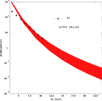
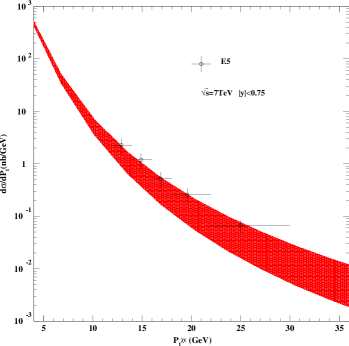
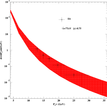
Since LO results obtained from the default choice of the LDME cannot provide good predictions, we shall give a range of the LDME to cover all the experimental data. Here we choose the range between the upper and lower bound of the values given in Eq.(17): . We can see in Fig.5 that the large band can cover most of the experimental data, and the upper bound overestimates the significance of feeddown contributions for some of the conditions. Still, we are not sure whether they are able to explain new experiments; however, a band presented for the range given above might cover the experimental data in the sense of statistics. And we know for sure that, a single value of the CO LDME cannot give reasonable predictions at LO.

At the end of this section, we present the values of the CO LDME at NLO for different choices of . For the same reason, we exclude E2 and E3 data. The LDMEs are listed as follows:
| (20) |
Here we have used renormalization scheme (in the calculation of NLO correction to the CO LDME). The are 0.48, 0.46, and 0.42, respectively.
Fitting experimental data at different ’s is actually an alternative procedure of solving the LDME running equation, which can be obtained from the renormalization of the LDME as
| (21) |
As Fig.2 shows, is almost a constant for the experimental conditions in the fit,so we can expect that the LDMEs listed above would be consistent with Eq.(21). From Fig.2 and Eq.(16), the typical value of is about 0.09 (at large ). Employing this value, we find that the LDMEs in Eq.(20) satisfy Eq.(21).
We also present here the LDME obtained with the inclusion of E2 and E3, and see whether the results change much:
| (22) |
where the subscript denotes the -cutoff renormalization scheme as well as , and the subscripts , and refer to the renormalization scheme, with being the corresponding values. The are 0.51, 0.52, 0.50, and 0.46, respectively. The difference between the LDMEs fitted by including and excluding E2 and E3 ranges from to . The difference increases as gets smaller, which is caused by the different behavior of for the four experimental conditions. Including E2 and E3 enhances the slightly, which is to say that theoretical prediction can fit E2 and E3 equally as well as it fits E1 and E4E6. Figure6 presents the comparison of theoretical predictions for the eight LDMEs to the experimental data. Actually, all the eight LDMEs result in good agreement with the experiment. For E1 and E4E6, the bands hold small as varies, while for E2 and E3, the bands get very large in high regions, which is to say for E1, E4E6, and the small region in E2 and E3, the dependence can be absorbed into the LDMEs, while in the large regions in E2 and E3, the problem of dependence becomes severe.
The values of at LO obtained in this paper, which range from 0.00013GeV3 to 0.00126GeV3, are smaller than those in Ref. Cho and Leibovich (1996b) ((0.003270.00043)GeV3), Ref. Braaten et al. (2000) ((0.00190.0002)GeV3), and Ref. Sharma and Vitev (2013) ((0.001870.00025)GeV3), which employed the data obtained through extrapolation carried out in Ref. Abe et al. (1997a). The NLO LDMEs are slightly different from those obtained in Refs. Ma et al. (2011c); Gong et al. (2013), which is due to the different parameter choices between our paper and those cited above. With the same parameter choice, we can obtain exactly the same LDMEs with Refs. Ma et al. (2011c); Gong et al. (2013).
V summary
In this paper, we calculated production cross sections and the ratio at hadron colliders, and compared the theoretical predictions with the experiment. We presented a detailed analysis on the CO LDMEs and found that, at LO, there does not exist any universal value of the CO LDME to explain all the experiments, while at NLO, the CO LDME obtained from a global fit is able to explain all the experimental data. At LO, we obtained the value of ranging from 0.13 to 1.26 when fitting individual experiments E1E6. The upper and lower bounds of result in quite a large band, which can cover most of the experimental data; however, the upper bound overestimates the significance of feeddown contributions for some of the experimental conditions. As for the NLO case, we carried out a global fit by using eight schemes. Each of them agree well with the experimental data. We also investigated the dependence of the results and found that, for E1, E4E6, and the small region in E2 and E3, the dependence on can be absorbed into the LDMEs, while for the large region in E2 and E3, the problem of dependence is relatively severe. One needs to resum the large log terms rising from large rapidity to achieve better results. Our work provides a strong support of the NRQCD effective theory.
Acknowledgments.—We thank Jian-Xiong Wang for helpful discussion. This work is supported by the National Natural Science Foundation of China (Grant No. 11405268).
References
- Bodwin et al. (1995) G. T. Bodwin, E. Braaten, and G. P. Lepage, Phys.Rev.D 51, 1125 (1995).
- Einhorn and Ellis (1975) M. Einhorn and S. Ellis, Phys.Rev.D 12, 2007 (1975).
- Ellis et al. (1976) S. Ellis, M. B. Einhorn, and C. Quigg, Phys.Rev.Lett. 36, 1263 (1976).
- Chang (1980) C.-H. Chang, Nucl.Phys. B172, 425 (1980).
- Berger and Jones (1981) E. L. Berger and D. L. Jones, Phys.Rev.D 23, 1521 (1981).
- Baier and Ruckl (1982) R. Baier and R. Ruckl, Nucl.Phys. B201, 1 (1982).
- Butenschoen and Kniehl (2012) M. Butenschoen and B. A. Kniehl, Phys.Rev.Lett. 108, 172002 (2012).
- Chao et al. (2012) K.-T. Chao, Y.-Q. Ma, H.-S. Shao, K. Wang, and Y.-J. Zhang, Phys.Rev.Lett. 108, 242004 (2012).
- Gong et al. (2013) B. Gong, L.-P. Wan, J.-X. Wang, and H.-F. Zhang, Phys.Rev.Lett. 110, 042002 (2013).
- Butenschoen and Kniehl (2011) M. Butenschoen and B. A. Kniehl, Phys.Rev.Lett. 106, 022003 (2011).
- Li and Wang (2014) R. Li and J.-X. Wang, Phys.Rev.D 89, 114018 (2014).
- Maltoni et al., (2006) F. Maltoni et al., Phys. Lett. B 638, 202 (2006).
- Feng et al. (2015) Y. Feng, J.-P. Lansberg, and J.-X. Wang, Eur. Phys. J. C 75, 313 (2015).
- Ma and Venugopalan (2014) Y.-Q. Ma and R. Venugopalan, Phys. Rev. Lett. 113, 192301 (2014).
- Hagler et al. (2001) P. Hagler, R. Kirschner, A. Schafer, L. Szymanowski, and O. V. Teryaev, Phys. Rev. Lett. 86, 1446 (2001).
- Shuvaev et al. (2015) A. G. Shuvaev, V. A. Khoze, A. D. Martin, and M. G. Ryskin, Eur. Phys. J. C 75, 616 (2015).
- Ma et al. (2011a) Y.-Q. Ma, K. Wang, and K.-T. Chao, Phys.Rev.Lett. 106, 042002 (2011a).
- Ma et al. (2011b) Y.-Q. Ma, K. Wang, and K.-T. Chao, Phys.Rev.D 84, 114001 (2011b).
- Aaij et al. (2012a) R. Aaij et al. (LHCb Collaboration), Eur.Phys.J.C 72, 2100 (2012a).
- Aaij et al. (2012b) R. Aaij et al. (LHCb Collaboration), Phys.Lett.B 718, 431 (2012b).
- Aaij et al. (2011) R. Aaij et al. (LHCb Collaboration), Eur.Phys.J.C 71, 1645 (2011).
- Cho and Leibovich (1996a) P. L. Cho and A. K. Leibovich, Phys.Rev.D 53, 150 (1996a).
- Cho and Leibovich (1996b) P. L. Cho and A. K. Leibovich, Phys.Rev.D 53, 6203 (1996b).
- Braaten et al. (2000) E. Braaten, B. A. Kniehl, and J. Lee, Phys. Rev.D 62, 094005 (2000).
- Sharma and Vitev (2013) R. Sharma and I. Vitev, Phys.Rev.C 87, 044905 (2013).
- Ma et al. (2011c) Y.-Q. Ma, K. Wang, and K.-T. Chao, Phys.Rev.D 83, 111503 (2011c).
- Li et al. (2011) D. Li, Y.-Q. Ma, and K.-T. Chao, Phys.Rev.D 83, 114037 (2011).
- Shao and Chao (2014) H.-S. Shao and K.-T. Chao, Phys.Rev.D 90, 014002 (2014).
- Shao et al. (2014) H.-S. Shao, Y.-Q. Ma, K. Wang, and K.-T. Chao, Phys.Rev.Lett. 112, 182003 (2014).
- Abulencia et al. (2007) A. Abulencia et al. (CDF Collaboration), Phys.Rev.Lett. 98, 232001 (2007).
- Aaij et al. (2012c) R. Aaij et al. (LHCb Collaboration), Phys.Lett.B 714, 215 (2012c).
- Chatrchyan et al. (2012) S. Chatrchyan et al. (CMS Collaboration), Eur.Phys.J.C 72, 2251 (2012).
- Likhoded et al. (2014) A. Likhoded, A. Luchinsky, and S. Poslavsky, Phys.Rev.D 90, 074021 (2014).
- Wang and Zhang (2015) J.-X. Wang and H.-F. Zhang, J. Phys.G 42, 025004 (2015).
- Petrelli et al. (1998) A. Petrelli, M. Cacciari, M. Greco, F. Maltoni, and M. L. Mangano, Nucl.Phys. B514, 245 (1998).
- Gong et al. (2011) B. Gong, J.-X. Wang, and H.-F. Zhang, Phys.Rev.D 83, 114021 (2011).
- Harris and Owens (2002) B. Harris and J. Owens, Phys.Rev.D 65, 094032 (2002).
- Wang (2004) J.-X. Wang, Nucl.Instrum.Methods Phys.Res.,Sect.A 534, 241 (2004).
- Eichten and Quigg (1995) E. J. Eichten and C. Quigg, Phys.Rev.D 52, 1726 (1995).
- Pumplin et al. (2002) J. Pumplin, D. Stump, J. Huston, H. Lai, P. M. Nadolsky et al., J.High Energy Phys. 07, 012 (2002).
- Xu et al. (2012) G.-Z. Xu, Y.-J. Li, K.-Y. Liu, and Y.-J. Zhang, Phys.Rev.D 86, 094017 (2012).
- Kang et al. (2014) Z.-B. Kang, Y.-Q. Ma, and R. Venugopalan, J.High Energy Phys. 01, 056 (2014).
- Abe et al. (1997a) F. Abe et al. (CDF Collaboration), Phys.Rev.Lett. 79, 578 (1997a).
- Abe et al. (1997b) F. Abe et al. (CDF Collaboration), Phys. Rev. Lett. 79, 572 (1997b).
- Aaij et al. (2013) R. Aaij et al. (LHCb Collaboration), J.High Energy Phys. 10, 115 (2013).
- Aad et al. (2014) G. Aad et al. (ATLAS Collaboration), J.High Energy Phys. 07, 154 (2014).
- Olive et al. (2014) K. Olive et al. (Particle Data Group), Chin.Phys.C 38, 090001 (2014).