Analysing oscillatory trends of discrete-state stochastic processes through HASL statistical model checking

Abstract

The application of formal methods to the analysis of stochastic oscillators has been at the focus of several research works in recent times. In this paper we provide insights on the application of an expressive temporal logic formalism, namely the Hybrid Automata Stochastic Logic (HASL), to that issue. We show how one can take advantage of the expressive power of the HASL logic to define and assess relevant characteristics of (stochastic) oscillators.

1 Introduction

Oscillations are a relevant type of dynamics which characterises the behaviour of several types of system in different domains, notably in the field of biological modelling.

The analysis of oscillations is a well established subject in applied mathematics for which different approaches exist. For example for systems described in terms of Ordinary Differential Equations (ODEs) limit-cycle analysis can be used to assess oscillation characteristics (e.g. period and amplitude of oscillations). On the other hand signal processing methods such as, for example, Fast Fourier Transformation (FFT) or autocorrelation analysis can be used to extract the oscillatory characteristic of a given signal, i.e. a sequence of points resulting from the observed system (being it the actual system under investigation or a model representing it).

In recent times the study of oscillatory systems has attracted the attention of research in the area discrete-state stochastic models (in the remainder we will refer to these kind of oscillatory models simply as stochastic oscillators) yielding to a number of research works aimed at the application of temporal logic reasoning to characterisation of oscillations [8, 25, 4, 12]. The goal in that respect is, quite simply, to adapt (stochastic) model checking techniques so that, given a model $M$, one is capable to obtain answers to questions such as: “does $M$ oscillates?” , “where the peaks of oscillations are located ?” “what is the (average) period of oscillations?”. Since here we refer to stochastic models answering such questions usually boils down to assessing some distribution of probability (e.g. assessing the steady-state distribution of $M$, and/or the PDF of the period duration, and/or the PDF of the location of the peaks of oscillations). So far analysis of oscillations through stochastic model checking have been mainly obtained through application of the Continuous Stochastic Logic (CSL) [5] (in some cases joint to its reward-based extensions [21]) approach or similarly expressive (linear-time) variants (e.g. Metric Interval Temporal Logic [12]). Interestingly, in recent times, Spieler [25] has shown how qualitative, such as “does a model $M$ oscillates sustainably?”, as well as quantitative, such as, for example, “what is the period of oscillation of a sustained oscillator $M$?”, queries can be formally assessed (in CSL form) by coupling a continuous-time Markov chain (CTMC) model with a timed automaton (TA) “monitor” capable of identifying noisy-periodic traces.

In this paper we extends Spieler’s approach by considering a recently introduced formalism, i.e. the Hybrid Automata Stochastic Logic (HASL) [7], as a means for studying stochastic oscillators.

Paper contribution.

The paper main contribution is one of demonstrating the effectiveness of the HASL formalism as a means to effectively specify and automatically estimate oscillation related measures. We consider two different approaches: the first concerned with assessing the oscillation period, the second concerned with measuring the oscillation peaks (hence the oscillation amplitude). We define two specific types of linear hybrid automata (LHA) that, when synchronised with an oscillatory stochastic process, are capable of detecting the periods, respectively the peaks, of its trajectories and compute on-the-fly classical characteristics like the average duration or the average amplitude of the oscillations as well as more sophisticated ones like the period fluctuation, which allow for assessing the regularity of an oscillator.

We demonstrate such contributions by considering a well-known case study. i.e. the analysis of a model of the circadian clock [26].

Paper organisation.

In Section 2 we introduce the HASL formalism. In Section 3 we describe the basic contribution of the paper, namely the application of HASL to the analysis of oscillations. In Section 4 we demonstrate the HASL-based analysis of oscillations on an example of biological oscillator. We wrap up the paper with some concluding remarks in Section 6.

2 HASL model checking

HASL framework belongs to the family of so-called statistical model checking methods, whose goal is to produce estimates of a (formally specified) target measure through sampling of the trajectories of the model. HASL is an automata-based type of logic, meaning that it employs automata, and specifically linear hybrid automata (LHA) as machineries for characterising the properties to be investigated. This yields the main feature of HASL, that is, its expressive power which in this paper we are going to demonstrate in respect to the oscillation analysis problem.

Simply speaking the HASL model checking procedure works as follows: given a model ${\cal D}$ and a certain dynamics of interest encoded by an LHA ${\cal A}$, the HASL model checker samples trajectories of the synchronised process ${\cal D}\!\times\!{\cal A}$, hence selecting only those paths of ${\cal D}$ that are accepted by ${\cal A}$ and using them for estimating the confidence-interval of a given target measure (in the following denoted $Z$), a quantity defined as a function of the LHA variables.

In the following we recall the basics formal elements for HASL: the characterisation of Discrete Event Stochastic Process (DESP) i.e the pertaining class of models, the characterisation of LHA and of the corresponding synchronised process ${\cal D}\!\times\!{\cal A}$, and that of target measure $Z$. For more details we refer the reader to [7].

2.1 Discrete Event Stochastic Processes

We refer to a DESP as a discrete-state stochastic process consisting of an enumerable set of states and whose dynamic is triggered by a set of (time consuming) discrete events. We do not consider any restriction on the nature of the distribution associated with events. Otherwise said a DESP is a family of random variables $\{X(t)\mid t\in\mathbb{R}_{\geq 0}\}$ representing time and where, in the context of this paper, $\mathbb{N}^{n}$ is assumed to be the support of $X$ (i.e. we talk in this case of an $n$-dimensional DESP population model, see Definition 3). Below we formally define the components a DESP consists of. Such characterisation is useful to provide an algorithmic formulation of the dynamics of a DESP (see below) which is at the basis of the HASL statistical model checking procedure.

Notation

For $A$ a generic set we denote $dist(A)$ the set of possible probability distributions whose support is $A$, that is, $dist(A)=\{\mu:\Sigma_{A}\to\mathds{R}^{+}|(A,\Sigma_{A},\mu)\}$ where $(A,\Sigma_{A},\mu)$ is a probability space. Observe that depending on the nature of $A$ the corresponding probability distributions $\mu\in dist(A)$ are either continuous (if $A$ is dense) or discrete (if $A$ is finite/discrete).

Definition 1 (DESP)

A DESP is a tuple
${\cal D}=\langle S,\pi_{0},E,Ind,enabled,delay,choice,target\rangle$ where

• $S$ is an enumerable (possibly infinite) set of states,

• $\pi_{0}\in dist(S)$ is the initial distribution on states,

• $E$ is a finite set of events,

• $Ind$ is a set of functions from $S$ to ${\mathds{R}}$ called state indicators (including the constant functions),

• $enabled\!:S\rightarrow 2^{E}$ are the enabled events in each state with for all $s\in S$, $enabled(s)\neq\emptyset$.

• $delay\!:S\times E\rightarrow dist(\mathds{R}^{+})$ is a partial function defined for pairs $(s,e)$ such that $s\in S$ and $e\in enabled(s)$.

• $choice\!:S\times 2^{E}\times\mathds{R}^{+}\rightarrow dist(E)$ is a partial function defined for tuples $(s,E^{\prime},d)$ such that $E^{\prime}\subseteq enabled(s)$ and such that the possible outcomes of the corresponding distribution are restricted to $e\in E^{\prime}$.

• $target\!:S\!\times\!E\!\times\mathds{R}^{+}\!\to\!S$ is a partial function describing state changes through events defined for tuples $(s,e,d)$ such that $e\!\in\!enabled(s)$.

A configuration of a DESP consists of a triple $(s\mathbin{,}\tau\mathbin{,}sched)$ with $s$ being the current state, $\tau\!\in\!{\mathds{R}}^{+}$ the current time and $sched:E\rightarrow{\mathds{R}}^{+}\cup\{+\infty\}$ being the function that describes the occurrence time of each scheduled event ($+\infty$ if an event is not yet scheduled). Observe that a scheduler $sched$ essentially describes the state of events’ queue in a given configuration of the DESP, thus all (currently) enabled events will have a finite scheduled time $sched(e)\!<\!\infty$, whereas non-enabled events will be associated with an infinite delay, that is, $sched(e)\!=\!\infty$. Thus, within the algorithm for generating a trajectory of a DESP, a scheduler $sched$ provides the occurrence time of the next event to occur (see also Algorithm 1). In the remainder we denote $Conf\!=\!S\!\times\!\mathds{R}^{+}\!\times\!Sched$ the set of possible configurations of a DESP (where $Sched$ denotes the set of possible schedules functions for the events of the DESP). Also for a configuration $c\!=\!(s\mathbin{,}\tau\mathbin{,}sched)\!\in\!Conf$, we denote $c(s)$, $c(\tau)$ and $c(sched)$ the state $s$, respectively the time $\tau$ and the schedule $sched$ of configuration $c$.

For a state $s$, $enabled(s)$ is the set of events enabled in $s$. For $e\!\in\!enabled(s)$, $delay(s,e)$ is the distribution of the delay between the enabling of $e$ and its possible occurrence. Furthermore, if we denote $\delta_{m}$ the delay of the earliest event in the current configuration $(s\mathbin{,}\tau\mathbin{,}sched)$ of the process, and $E_{min}\!\subseteq\!enabled(s)$ the set of events with earliest delay, then $choice(s,E_{min},\delta_{m})$ describes how the conflict between the concurrent events in $E_{min}$ is randomly resolved: i.e. $choice(s,E_{min},\delta_{m})(e^{\prime})$ is the probability that $e^{\prime}\!\in\!E_{min}$ will be selected hence occurring with delay $\delta_{m}$. Finally function $target(s,e,d)$ denotes the target state reached from $s$ on occurrence of $e$ after waiting for $d$ time units.

Dynamics of a DESP.

The evolution of a DESP ${\cal D}$ can be informally summarised by an iterative procedure consisting of the following steps (assuming $(s\mathbin{,}\tau\mathbin{,}sched)$ is the current configuration of ${\cal D}$): 1) determine the set $E_{min}$ of events enabled in state $s$ and with minimal delay $\delta_{m}$; 2) select the next event to occur $e_{next}\!\in\!E_{min}$ by resolving conflicts (if any) between concurrent events through probabilistic choice according to $choice(s,E_{min},\tau)$; 3) determine the new configuration of the process resulting from the occurrence of $e_{next}$, this in turns consists of three sub-steps: 3a) determine the new state resulting from occurrence of $e_{next}$, i.e. $s^{\prime}=target(s,e_{next},\delta_{m})$; 3b) update the current time to account for the delay of occurrence of $e_{next}$, i.e. $\tau=\tau+\delta_{m}$; 3c) update the schedule of events according to the newly entered state $s^{\prime}$ (this implies setting the schedule of no longer enabled events to $+\infty$ as well as determining the schedule of newly enabled events by sampling through the corresponding distribution). Such procedure is (semi-formally) summarised in Algorithm 1.

Algorithm 1 Evolution of a DESP

  initial_configuration: $(s\mathbin{,}\tau\mathbin{,}sched)$

  while $Enabled(s)\neq\emptyset$ do

     $E_{min}\!=\!min(\cup_{e\in enabled(s)}sched(e))$

     $e_{next}=choice(s,E_{min},\tau)$

     $\delta_{m}=sched(e_{next})$

     $s^{\prime}=target(s,e_{next},\delta_{m})$

     $\tau^{\prime}=\tau+\delta_{m}$

     $sched(e)\!=+\infty$  ($\forall e\!\not\in\!enabled(s^{\prime}))$

     $sched(e)\!=\!sample(delay(s^{\prime},e))$  ($\forall e\!\in\!enabled(s^{\prime}))$

A path (or trajectory) of a DESP is a sequence of configurations $\sigma\!=\!c_{1},c_{2},c_{3},\ldots$ resulting from the execution of the procedure highlighted by Algorithm 1. We formalise this in the following definition. The notion of DESP path will be used later on for reasoning about the dynamics of a DESP and in particular for reasoning about oscillations.

Definition 2 (Path of a DESP)

For a DESP ${\cal D}=\langle S,\pi_{0},E,Ind,enabled,delay,choice,target\rangle$ with $Conf$ the set of its configurations we define the set of finite paths as $Path^{*}\subseteq\bigcup_{n\!\in\!\mathds{N}}Conf^{n}$. We denote $\sigma\!=\!(c_{0},c_{1}\ldots,c_{n})\!\in\!Path^{*}$, where $\pi_{0}(c_{0}(s))\!>0$ and $\forall 0\leq i<n$, $\exists e\!\in\!E_{min}(c_{i}(s))$ such that $c_{i+1}(s)=target(c_{i}(s),e,c_{i}(\tau))$. By extension we denote $Path^{\omega}$ as the set of infinite path and $Path\!=\!Path^{*}\!\cup\!Path^{\omega}$ as the of all paths of a DESP.

In the remainder we might refer to a DESP path using $\sigma\!=\!(c_{0},c_{1}\ldots,c_{n})$ or, depending on the context, simply indicating the corresponding sequence of states $\sigma\!=\!(c_{0}(s),c_{1}(s)\ldots,c_{n}(s))$, or simply $\sigma\!=\!(s_{0},s_{1}\ldots,s_{n})$. Furthermore for a path $\sigma\!=\!(c_{0},c_{1}\ldots,c_{n})$ we use the following notations: for $i\!\in\!\mathds{N}$, $\sigma[i]=c_{i}(s)$ denotes the $i$-th state, while for $t\!\in\!\mathds{R}^{+}$, $\sigma@t$ denotes the state in which $\sigma$ is at time $t$, that is, $\sigma@t\!=\!\sigma[i]$ such that $i$ is the smallest $i$ with $t\!\leq\!c_{i}(\tau)$

Since in this paper we deal with the analysis of discrete-state biological models representing the evolution of the molecular population of $n$ species, we introduce the notion of DESP population model.

Definition 3 (DESP Population Model)

A DESP model for $n\!\in\!\mathds{N}$ population types is a DESP ${\cal D}=\langle S,\pi_{0},E,Ind,enabled,delay,choice,target\rangle$ with $S\!\subseteq\!\mathds{N}^{n}$.

Definition 4 (DESP Observed Species)

For ${\cal D}$ a DESP population model with $n$ species we define ${\cal D}_{i}$ the observed $i^{th}$ process, with $1\!\leq\!i\!\leq\!n$, as the process resulting from ${\cal D}$ by observing only the $i^{th}$ component of each state of ${\cal D}$. Thus each $s\!=\!(s_{1},\ldots,s_{i},\ldots s_{n})\!\in\!S$ of ${\cal D}$ corresponds to state $s_{i}\!\in\!S_{i}$ of ${\cal D}_{i}$.

By extension for $\sigma\!\in\!Path$ a path of a DESP population model we denote $\sigma_{i}$ the $i^{th}$ projection of $\sigma$, thus if $\sigma\!=\!(s^{1}_{0},\ldots s^{n}_{0}),(s^{1}_{1}\ldots s^{n}_{1}),\ldots$ then $\sigma_{i}\!=\!s^{i}_{0},s^{i}_{1}\ldots$

Indicator functions.

In the definition of DESP we include a set of indicator functions denoted $Ind$. An indicator $\alpha\!\in\!Ind$ maps states of a DESP to real values $\alpha:S\to{\mathds{R}}$. DESP indicators describe what information can be seen by an LHA during the synchronisation with a DESP. Specifically, indicators appear in various parts of a synchronising LHA (see Definition 5): in the location invariants (function $\Lambda$), in a location’s flow, and in the edge constraints ($\mathsf{Const}$ and $\mathsf{lConst}$, within $\to$) and edge updates ($\mathsf{Up}$) of an LHA edge. We denote $Prop\!\subseteq\!Ind$ the subset of boolean valued indicators called propositions, i.e., for $\alpha^{*}\!\in\!Prop$, $\alpha^{*}:S\to\{0,1\}$. Indicators are evaluated against states. Thus for $s\!\in\!S$, and $\alpha\!\in\!Ind$ an indicator, $\alpha(s)$ denotes the value of $\alpha_{i}$ in state $s$. Specific details about how indicators are applied within the characterisation of an LHA are given in Section 2.2.

DESP in terms of GSPN

For implementation convenience, in the context of HASL and in particular of the associated model checking tool C OSMOS  [1, 6], we represent DESP models in terms of stochastic petri nets, and more precisely we adopt (the non-markovian extension of) Generalised Stochastic Petri Net (GSPN) [2] as the high-level input formalism for expressing a DESP model. Thus, in this context, DESP indicators are actually GSPN indicators, that is: they are expressions which contain references to the (marking of the) places of a GSPN model. For the sake of brevity here we assume familiarity with the GSPN formalism, referring the reader to the literature [2] for details. GSPN semantics is briefly presented later on through description of a simple GSPN model (see Figure 1).

Example: DESP indicators within LHA.

In the LHA of Figure 1 (right) the indicator protA, which refers to the marking of the GSPN place named protA in Figure 1 (left), is used within the updates of the self-loop edges of location $l_{0}$. Specifically indicator protA is used to update the LHA variable $a$ with the current number of tokens contained in GSPN place protA. Similarly in the LHA of Figure 4 the GSPN place indicator $A$ (which refers to the GSPN place named $A$ of the GSPN in Figure 8) is used within the invariant constraints $A\!\leq\!L$, $L\!\leq\!A\!\leq\!H$ and $A\!\geq\!H$ associated respectively with locations $low$, $mid$ and $high$ (where $L,H\!\in\!\mathds{R}$ are just symbolic names for two real-valued constants used for representing a generic version of the ${\cal A}_{per}$ LHA: in practice concrete instances of ${\cal A}_{per}$ are obtained by actual instances of $L,H$, e.g., $L\!=\!1$ and $H\!=\!10$). Such invariants essentially state that entering the locations $low$, $mid$ and $high$ depend on the current marking of place $A$ (see Section 3.1 for more details).

2.2 Hybrid Automata Stochastic Logic

The Hybrid Automata Stochastic Logic, introduced in [7], extends Deterministic Timed Automata (DTA) logics for describing properties of Markov chain models [13, 10], by employing LHA (a generalisation of DTA) as instruments for characterising specific dynamics of an observed DESP model. An HASL formula consists of two elements: 1) a so-called synchronising LHA, i.e. an LHA enriched with (state and/or event) indicators of the observed DESP and 2) a target expression (see grammar (1)) which expresses the quantity to be evaluated. The synchronised LHA is used for selecting the trajectories that correspond to the behaviour to of interest. The target expression indicates what statistics, i.e. what function of the synchronised LHA data variables, will be assessed with respect to the trajectories selected by the LHA.

In the following we formally introduce the notion of synchronised LHA and then informally describe the stochastic process resulting from the product of a DESP and a synchronised LHA.

Definition 5

A synchronised linear hybrid automaton is a tuple $\mathcal{A}\!=\!\langle E,L,\Lambda,I,F,X,\textit{flow},\rightarrow\rangle$ where:

• $E$ is a finite alphabet of events;

• $L$ is a finite set of locations;

• $\Lambda:L\rightarrow Prop$ is a location labelling function;

• $I\subseteq L$ is the initial locations;

• $F\subseteq L$ is the final locations;

• $X=(x_{1},...x_{n})$ is a $n$-tuple of data variables;

• $\textit{flow}:L\mapsto Ind^{n}$ associates an $n$-tuple of indicators with each location (the $i^{th}$ projection $\textit{flow}_{i}$ denotes the flow of change of variable $x_{i}$).

• $\rightarrow\subseteq L\times\left((2^{E}\times\mathsf{Const})\uplus(\{\sharp\}\times\mathsf{lConst})\right)\times\mathsf{Up}\times L$ is the set of edges of the LHA ,

where $\uplus$ denotes the disjoint union, $\mathsf{Const}$ and $\mathsf{lConst}$ denotes the set of possible constraints, respectively left closed constraints, associated with ${\cal A}$ (see details below), $\mathsf{Up}$ is the set of possible updates for the variables of ${\cal A}$ and $Prop\!\subseteq\!Ind$ denotes the subset of boolean valued DESP indicators.

Before presenting informally the synchronisation of a DESP with an LHA we start by describing the various parts of an LHA. In what follows we denote indicators symbolically by greek letters $\alpha,\alpha^{\prime}\!\in\!Ind$, while we use capital letters $A,B,\ldots$ to refer to names of GSPN places (within concrete indicators instances) and $x_{1},x_{2},\ldots$ to denote LHA variables. Thus, for example, $\alpha\!\equiv\!A+2B$ is an indicator whose value is given by the sum of the marking of place $A$ with twice the marking of place $B$.

Location proposition:

function $\Lambda$ associates each location $l\!\in\!L$ with a proposition (also called location invariant in the remainder) $\Lambda(l)\!\in\!Prop$ representing a condition under which a location can be entered. A location proposition consists of a boolean combination of inequalities involving DESP indicators and has the following form $\Lambda(l)\!\equiv\!\bigwedge_{i}(\!\alpha_{i}\!\prec\!\alpha^{\prime}_{i}\!)$ with $\alpha_{i},\alpha^{\prime}_{i}\!\in\!Ind$, and $\prec\in\!\{=,<,>,\leq,\geq\}$. Notice that indicators can be constant functions, thus, for example, a location proposition may consist of comparing indicators’ values against constant thresholds, as in, e.g., $\Lambda(l)\!\equiv\!A\!\!\geq\!10$, or it may consist of comparing different indicators one another, as in, e.g., $\Lambda(l)\!\equiv\!A\!\leq\!B$ or $\Lambda(l)\!\equiv\!A\!\leq\!B^{2}\sqrt{C}$. A location proposition (given by $\Lambda$) is shown by a label next to the location it refers to. For convenience no label is shown next to unconstrained locations, i.e., locations associated to a tautology like $\top\equiv(\alpha_{i}\!=\!\alpha_{i})$. Location propositions are evaluated against states of a DESP. Thus for $s\!\in\!S$ a DESP state and $l\!\in\!L$ a location of an LHA we say that $s$ satisfies the invariant $\Lambda(l)$, denoted $s\!\models\!\Lambda(l)$, if $\Lambda(l)(s)\!=\!{\bf true}$ (where $\Lambda(l)$ is the value of the boolean expression obtained by replacing each indicator $\alpha\!\in\!\Lambda(l)$ with its value $\alpha(s)$). Furthermore given two edge locations $l$ and $l^{\prime}$ we say that the their respective invariants are inconsistent, denoted $\Lambda(l)\land\Lambda(l^{\prime})\Leftrightarrow\mbox{\tt false}$, if there cannot exist a state $s$ that satisfies $\Lambda(l)\land\Lambda(l^{\prime})$. For example, if $\Lambda(l)\!\equiv\!A\!\leq\!2$ and $\Lambda(l^{\prime})\!\equiv\!A\!>\!2$ then trivially $A\!\leq\!2\land A\!>\!2\Leftrightarrow\mbox{\tt false}$. This means that $l$ and $l^{\prime}$ are mutually exclusive, which is a necessary condition for LHA with multiple initial locations (see conditions c1 below).

Edge constraint:

edge constraints describe necessary conditions for an edge to be traversed. We denote $\mathsf{Const}$ (resp. $\mathsf{lConst}$) the set of constraints (resp. left-closed constraints) of an LHA edge. An edge constraint consists of a boolean combination of inequalities involving both DESP indicators and LHA variables. They have the following form $\gamma\!\equiv\!\bigwedge_{j}(\sum_{1\leq i\leq n}\alpha_{ij}x_{i}\!\prec\!\alpha^{\prime}_{j}\!)$ with $\alpha_{ij},\alpha^{\prime}_{j}\!\in\!Ind$, $x_{i}\!\in\!X$ and $\prec\in\!\{=,<,>,\leq,\geq\}$. Simple examples of edge constraints can be: $\gamma\!\equiv(2x_{1}\!+\!3x_{2}\!\leq\!5)$ or also $\gamma\!\equiv(Ax_{1}\!=\!5)$. Given a location $l$ of the LHA and a state $s$ of the DESP, the inequalities $\gamma_{j}\!\equiv\!\sum_{1\leq i\leq n}\alpha_{ij}x_{i}\!\prec\!\alpha^{\prime}_{j}$ a constraint $\gamma$ consists of evolve linearly with time hence each inequality gives an interval of time during which the constraint $\gamma$ is satisfied. We say that a constraint is left closed if, whatever the current state $s$ (defining the values of the DESP indicators), the time at which the constraint is satisfied is a union of left closed intervals (for example, $\gamma\!\equiv(x_{1}\!\geq\!5)$ is left-closed whereas $\gamma\!\equiv(x_{1}\!>\!5)$ is not). We denote $\mathsf{lConst}\!\subseteq\!\mathsf{Const}$ the subset of left-closed constraint. For efficiency the constraint of autonomous-edges (see below) must be left-closed.

Edge constraints are evaluated against pairs $(s,\nu)\!\in\!S\!\times\!Val$ where $s\!\in\!S$ is a state of a DESP and $\nu:X\rightarrow\mathds{R}\!\in\!Val$ is a valuation that maps every LHA data variable to a real value (we denote $Val$ the set of all possible valuations). For $\nu\!\in\!Val$, $\nu(x)$ denotes the value of variable $x$ through valuation $\nu$. Given $\gamma_{j}\!\equiv\!\sum_{1\leq i\leq n}\alpha_{ij}x_{i}\!\prec\!\alpha_{j}$ an inequality contained in an edge-constraint $\gamma\!\equiv\!\bigwedge_{j}\gamma_{j}$, its interpretation w.r.t. $\nu$ and $s$, denoted $\gamma_{j}(s,\nu)$, is defined by $\gamma_{j}(s,\nu)=\sum_{1\leq i\leq n}\alpha_{ij}(s)\nu(x_{i})\!\prec\!\alpha^{\prime}_{j}(s)$. We write $(s,\nu)\models\gamma_{j}$ if $\gamma_{j}(s,\nu)\!=\!{\bf true}$ and, by extension, $(s,\nu)\models\gamma$ iff $(s,\nu)\models\gamma_{j}$ for all $j$. Furthermore given two edge constraints $\gamma$ and $\gamma^{\prime}$ we say that their conjunction $\gamma\land\gamma^{\prime}$ is inconsistent, denoted $\gamma\land\gamma^{\prime}\Leftrightarrow\mbox{\tt false}$, if there exists no combination $(s,\nu)\!\in\!S\!\times\!Val$ that satisfies it. For example, if $\gamma\!\equiv\!x_{1}\!\leq\!2$ and $\gamma^{\prime}\!\equiv\!x_{2}\!>\!2$ are the constraints for two edges then trivially $(x_{1}\!\leq\!2)\land(x_{1}\!>\!2)\Leftrightarrow\mbox{\tt false}$, meaning the two edges cannot be concurrently enabled (see conditions c2 and c3 below).

Edges update:

an edge update $U\!=\!(u_{1},...,u_{n})\!\in\!Up$ is an $n$-tuple of functions characterising how each LHA variable $x_{k}$ is going to be updated on traversal of the edge. Each function $u_{k}$ ($1\!\leq\!k\!\leq\!n$) of an edge update $U\!=\!(u_{1},...,u_{n})\!\in\!Up$ is of the form $x_{k}=\sum_{1\leq i\leq n}\alpha_{i}x_{i}+c$ where the $\alpha_{i}$ and $c$ are DESP indicators. Similarly to edge constraints, updates are evaluated against pairs $(s,\nu)\!\in\!S\!\times\!Val$. Given an update $U=(u_{1},\ldots,u_{n})$, we denote by $U(s,\nu)$ the valuation defined by $U(s,\nu)(x_{k})=u_{k}(s,\nu)$ for $1\leq k\leq n$.

Locations flow:

a location flow is an $n$-tuple of indicators $flow(l)\!=\!(\alpha_{1},\ldots,\alpha_{n})$, where $\alpha_{i}\!\in\!Ind$ describes the gradient at which variable $x_{i}\!\in\!X$ changes while the automaton sojourns in location $l$. Specifically when location $l$ is entered the rate of change of each $x_{i}$ is established by the valuation, w.r.t. to the state the DESP is at on entering of $l$, of the corresponding $\alpha_{i}$. Observe that, if each $\alpha_{i}$ in $flow(l)$ is a constant function (e.g. $\alpha_{i}=c_{i}$, with $c_{i}\!\in\!\mathds{R}$) then each variable $x_{i}$ changes at constant rate throughout the sojourn in $l$. However this is not necessarily the case for variables whose flow is given by a non-constant indicator, like, for example, $\alpha_{i}\!=\!c_{1}A+c_{2}B$, with $c_{1},c_{2}\!\in\!\mathds{R}$ and $A,B$ representing the marking of two GSPN places named $A$ and $B$. In this case the flow of change of $x_{i}$ depends on the marking of places $A$ and $B$, and such marking may change during the sojourn in $l$, for example if a synchronising self-loop edge $l\to l$ exists which synchronises with some DESP event whose occurrence modify the marking of $A$ or $B$.

Having described the DESP indicators dependent elements of an LHA we now see how they are all combined within the characterisation of an LHA edge.

Edges of an LHA.

An edge $l\xrightarrow{E^{\prime},\gamma,U}l^{\prime}$ of an LHA is labelled by: 1) a constraint $\gamma$, 2) a set of event labels $E^{\prime}$, 3) an update $U$. An edge can be either synchronous or autonomous. A synchronous edge is one whose traversal is triggered by the occurrence of an event of the DESP in particular an event $e\!\in\!E^{\prime}\!\subseteq E$ where $E^{\prime}$ is the set of event names labeling the edge. An autonomous edge, on the other hand, is one whose traversal is independent of the occurrence of DESP events, hence the event label for autonomous edges is $E^{\prime}\!\equiv\!\sharp$, where $\sharp$ is the label used for representing a “pseudo-event”.

The class of LHA for HASL is further restrained by the following conditions:

• c1 (initial determinism): $\forall l\neq l^{\prime}\!\in\!I$, $\Lambda(l)\wedge\Lambda(l^{\prime})\Leftrightarrow\mbox{\tt false}$. This means that independently of the interpretation of the indicators, hence of the synchronising DESP model, at most one initial location $l\!\in\!I$ can have its constraint $\Lambda(l)$ verified.

• c2 (determinism on events:) $\forall E_{1},E_{2}\!\subseteq\!E$ $:\!E_{1}\!\cap\!E_{2}\neq\emptyset,$ $\forall l,l^{\prime},l^{\prime\prime}\in L,$ if $l^{\prime\prime}\xrightarrow{E_{1},\gamma,U}{l}$ and $l^{\prime\prime}\xrightarrow{E_{2},\gamma^{\prime},U^{\prime}}{l^{\prime}}$ are two distinct transitions, then either $\Lambda(l)\wedge\Lambda(l^{\prime})\Leftrightarrow\mbox{\tt false}$ or $\gamma\wedge\gamma^{\prime}\Leftrightarrow\mbox{\tt false}$. Again this equivalence must hold whatever the interpretation of the indicators occurring in $\Lambda(l)$, $\Lambda(l^{\prime})$, $\gamma$ and $\gamma^{\prime}$.

• c3 (Determinism on $\sharp$:) $\forall l,l^{\prime},l^{\prime\prime}\in L,$ if $l^{\prime\prime}\xrightarrow{\sharp,\gamma,U}{l}$ and $l^{\prime\prime}\xrightarrow{\sharp,\gamma^{\prime},U^{\prime}}{l^{\prime}}$ are two distinct transitions, then either $\Lambda(l)\wedge\Lambda(l^{\prime})\Leftrightarrow\mbox{\tt false}$ or $\gamma\wedge\gamma^{\prime}\Leftrightarrow\mbox{\tt false}$.

• c4 (no $\sharp$-labelled loops:) For all sequences
  $l_{0}\xrightarrow{E_{0},\gamma_{0},U_{0}}l_{1}\xrightarrow{E_{1},\gamma_{1},U_{1}}\cdots\xrightarrow{E_{n-1},\gamma_{n-1},U_{n-1}}{l_{n}}$ such that $l_{0}=l_{n}$, there exists $i\leq n$ such that $E_{i}\neq\sharp$.

Synchronisation of LHA and DESP.

The role of a synchronised LHA ${\cal A}$ is to select specific trajectories of a corresponding DESP ${\cal D}$ while collecting relevant data (maintained in the LHA variables) along the execution. Synchronisation is technically achieved through the product process ${\cal D}\times{\cal A}$ whose formal characterisation, for the sake of brevity, we omit in this paper: we provide however an intuitive description of the ${\cal D}\times{\cal A}$ semantics.

The product ${\cal D}\!\times\!{\cal A}$ is itself a DESP whose states are triples $(s,l,\nu)$ where $s$ is the current state of the ${\cal D}$, $l$ the current location of the ${\cal A}$ and $\nu\!:\!X\!\to\mathbb{R}$ the current valuation of the variables of ${\cal A}$. Formally the set of states of the product process ${\cal D}\!\times\!{\cal A}$ is defined as $S^{\prime}=(S\times L\times Val)\uplus\{\bot\}$, where $Val$ denotes the set of possible variables’ valuations and $\bot$ denotes the rejecting state, i.e., the state entered when synchronisation fails, hence when a trajectory is rejected (see below). Notice that a configuration of the product DESP ${\cal D}\times{\cal A}$ has the following form $((s,l,\nu),\tau,sched^{\prime})$, where $(s,l,\nu)$ is the current state of ${\cal D}\times{\cal A}$, $\tau\!\in\!{\mathds{R}}^{+}$ is the current time, and $sched^{\prime}$ is the schedule of the enabled events of ${\cal D}\times{\cal A}$. The synchronisation starts from the initial state $(s,l,\nu)$, where $s$ an the initial state of the DESP (i.e. $\pi_{0}(s)>0$), $l$ is an initial location of the LHA (i.e. $l\!\in\!I$) and the LHA variables are all initial set to zero (i.e. $\nu=0$).

From the initial state the synchronisation process evolves through transitions where each transition corresponds to traversal of either a synchronised or an autonomous edge of the LHA. Furthermore if an autonomous and a synchronised edge are concurrently enabled the autonomous transition is taken first. Let us suppose that $(s,l,\nu)$ is the current state of process ${\cal D}\!\times\!{\cal A}$ and describe how the synchronisation evolves. If in the current location of the LHA (i.e. location $l$ of the current state $(s,l,\nu)$) there exists an enabled autonomousedge $l\xrightarrow{\sharp,\gamma,U}l^{\prime}$, then that edge will be traversed leading to a new state $(s,l^{\prime},\nu^{\prime})$ where the DESP state ($s$) is unchanged whereas the new location $l^{\prime}$ and the new variables’ valuation $\nu^{\prime}$ might differ from $l$, respectively $\nu$, as a consequence of the edge traversal. On the other hand if an event $e$ of process ${\cal D}$ (corresponding to transition $s\xrightarrow{e}s^{\prime}$ of ${\cal D}$) occurs in state $(s,l,\nu)$, either an enabled synchronous edge $l\xrightarrow{E^{\prime},\gamma,U}l^{\prime}$ (with $e\!\in\!E^{\prime}$) exists leading to new state $(s^{\prime},l^{\prime},\nu^{\prime})$ of process ${\cal D}\!\times\!{\cal A}$ (from which synchronisation will continue) or the synchronisation halts hence the trace is rejected (formally this is achieved with the system entering the rejecting state $\bot$).

Enabling of an LHA edge.

Let us briefly describe how the enabling, hence the traversal, of an LHA edge is established. Let $(s,l,\nu)$ be the current state of process ${\cal D}\!\times\!{\cal A}$. An edge $l\xrightarrow{E,\gamma,U}l^{\prime}$ being it autonomous or synchronous originating in $l$ is enabled if the following two conditions hold: 1) if the edge constraint is satisfied in state $(s,l,\nu)$ (i.e., if $(s,\nu)\models\gamma$) 2) if the location invariant of the target location $\Lambda(l^{\prime})$ is satisfied in the state $s^{\prime}$ reached by traversal of the edge, i.e., if $s^{\prime}\!\models\!\Lambda(l^{\prime})$ (observe that if the considered edge is autonomous then necessarily $s^{\prime}\!=\!s$, whereas if it is synchronous then possibly $s^{\prime}\!\neq s$). Finally for a synchronous edge to be enabled, in addition to 1) and 2), it must be the case that the DESP event $e$ occurring while in $(s,l,\nu)$ is captured by the the edge, i.e., $e\!\in\!E$.

Remarks.

The above described synchronisation of a DESP and an LHA, which HASL model checking is based on, requires certain properties to hold, namely: uniqueness, convergence and termination of the synchronisation. This means that for ${\cal A}$ a synchronised LHA then for any (infinite) path $\sigma$ of a synchronising DESP model: 1) there must be exactly one synchronisation with ${\cal A}$, 2) synchronisation cannot go on indefinitely due to an infinity of consecutive autonomous events, 3) path $\sigma$ should lead to an absorbing state (i.e. a final location of the ${\cal A}$ or the rejecting state $\bot$) with probability 1. The uniqueness property is guaranteed by constraint c1, c2 and c3 of the LHA definition whereas convergence is a consequence of constraint c4. On the other hand termination of the synchronisation is not explicitly guaranteed, however can be ensured by structural properties of $\mathcal{A}$ and/or $\mathcal{D}$.

Example (synchronisation of DESP and LHA): To understand how synchronisation of a DESP with an LHA works let us consider a simple example. Figure 1 depicts a toy DESP model in GSPN form (on the left) coupled with a simple LHA (on the right). The GSPN model represents the basic steps of gene expression: 1) binding/unbinding of an activator protein to the promoter of $gene\_A$; 2) of transcription of a gene into an mRNA molecule; 3) degradation of the mRNA 4) translation of the mRNA into the expressed protein $prot\_A$. The states of the DESP consist of 4-tuples $s\!=\!$ (protA, geneA ,A_geneA, mrnA) $\!\in\!\mathds{N}^{4}$, corresponding to the marking of the 4 places of the GSPN, whereas the event set is $E\!=\!\{bind,unbind,degrade,transc,transl\}$, corresponding to the 5 timed-transitions of the GSPN. The LHA ${\cal A}$, on the other hand, consists of: two locations, $l_{0}$ (initial) and $l_{1}$ (final), and three data variables $t$ (a clock), $n$ (for counting the number of occurrences of the $transc$ event) and $a$ (for keeping track of the population of $prot\_A$). Notice that the invariant of both locations is $\Lambda(l_{0})\!=\!\Lambda(l_{1})\!=\!\top$, (hence no label is associated to $l_{0}$, $l_{1}$), meaning that both locations can be entered without constraint. The initial state of the product process ${\cal D}\times{\cal A}$ is $s_{0}\!=\!((2,1,0,0),l_{0},\nu_{0})$, where $\nu_{0}$ is the zero valuation (i.e., $\nu_{0}(t)\!=\!\nu_{0}(n)\!=\!\nu_{0}(a)\!=\!0$). ${\cal A}$ has two synchronised (self-loop) edges $l_{0}\xrightarrow{\{transc\},n\!<N,\{n++,a=\text{{protA}}\}}l_{0}$, which synchronises with occurrences of the $transc$ event, and $l_{0}\xrightarrow{E\setminus\{transc\},n\!<N,\{a=\text{{protA}}\}}l_{0}$, which synchronises with occurrences of any other event but $transc$ (i.e., $E\setminus\{transc\}$). The constraint for both synchronised edges is $n<N$ which means they can be traversed as long as the number of observed occurrences of $transc$, which is stored in $n$, is less than $N$. Both updates for the two synchronised edges refer to a single indicator, namely protA, whose value is given by the marking of the GSPN place labelled protA, but they are slightly different. The update for the edge which synchronises with $transc$ is $\{n\!+\!+,a=\text{{protA}}\}$, meaning that whenever the edge is traversed (i.e., on occurrence of a $transc$ event) the counter $n$ is incremented and the current marking of place protA is stored in $a$. On the other hand the update for the edge which synchronises with $E\setminus\{transc\}$ the update is simply $\{a=\text{{protA}}\}$ as clearly $n$ must be incremented only on occurrence of $transc$. Furthermore ${\cal A}$ has an autonomous edge $l_{0}\xrightarrow{\sharp\!,\!(\boldsymbol{n\!=\!N})\!,\!\emptyset}l_{1}$ leading to the final location $l_{1}$. Such edge gets enabled as soon as its constraint $(n\!=\!N)$ is satisfied, that is, as soon as a state $s_{N}\!=\!((n_{1},n_{2},n_{3},n_{4}),l_{0},\nu_{N})$, is reached with $\nu_{N}$ being a valuation such that $\nu_{N}(n)\!=\!N$. In any such state $s_{N}$ the autonomous edge is traversed (leading to state $s_{stop}\!=\!((n_{1},n_{2},n_{3},n_{4}),l_{1},\nu_{N})$) and the synchronisation stops.

Figure 1: Synchronisation between a DESP toy model (left) representing basic steps of gene expression and an LHA (right) which selects paths containing $N$ occurrences of the transcription event

HASL expressions.

The second component of an HASL formula is an expression related to the automaton. Such an expression, denoted $Z$, is defined by a specific grammar [7] of which here we consider only the basic elements given in (1).

$$\begin{split}Z::=&\ E[Y]\ |\ P\\ Y::=&\ last(y)\ |\ min(y)\ |\ max(y)\ |\ avg(y)\\ y::=&\ c\ |\ x\ |\ y+y\ |\ y\times y\ |\ y/y\end{split}$$ (1)

$Z$ is either either an expectation expression $E[Y]$, or a probability expression $P$. An expectation expression $Z=E[Y]$ represents the expected value of a random variable $Y$ built on top of basic path operators ($last(y)$, $min(y)$, $max(y)$ , $avg(y)$). Each such path operator take as argument $y$ an algebraic combination of the LHA data variables $x$, and is evaluated along a (synchronised) path that is accepted by the automaton. Intuitively the meaning of path operators is as follows: $last(y)$ represents the value that expression $y$ has at the instant a path is accepted, while $min(y)$ ($max(y)$, respectively $avg(y)$) represents the minimum (maximum, respectively average) value assumed by $y$ along an accepted path. Expression $Z\!=\!P$, on the other hand, simply represents the probability that a path is accepted by the LHA. This is given by the ratio between the number of accepted paths and total number of paths generated throughout a simulation experiment.

In recent updates the COSMOS model checker [6] has been enriched with facilities for assessing the Probability (Cumulative) Distribution Function (PDF, respectively CDF) of the value that an expression $Y$ takes at the end of a synchronising path. Notice that PDF and CDF HASL expressions, are only high-level macros supported by the COSMOS tool in order to give the user the possibility to straightforwardly specify PDF/CDF measures. Thus COSMOS supports the following syntax for estimating a PDF measure: $Z=PDF(Y,s,l,h)$, where $Y$ is the path dependent expression whose PDF is to be estimated while $l$ and $h$ are the lower, respectively higher, bound of the interval representing the support of $Y$ (i.e. estimation of the PDF of $Y$ is done assuming $Y$ takes value in $[l,y]$) and $s\!<\!(h-l)$ is the width of each sub-interval in which the considered support $[l,y]$ is discretised. Thus during estimation of $Z=PDF(Y,s,l,h)$ COSMOS internally maintains a counter for each of the $(h-l)/s$ sub-intervals. Each such counter is incremented if the value of $Y$ on acceptance of a trace falls in the corresponding sub-interval. Then the value returned by COSMOS for $Z=PDF(Y,s,l,h)$ is the array of frequencies obtained by dividing each of the above counters by the total number of generated trajectories.

Example

Having introduced the HASL expression we can now consider some examples of complete HASL formula referred to the model of Figure 1.

• $\phi_{1}\!\equiv\!({\cal A},E[last({t})])$: representing the average time for completing $N$ transcriptions

• ${\phi_{2}\!\equiv\!({\cal A},E[max({a})])}$: representing the maximum population reached by protein A within the first $N$ transcriptions

• ${\phi_{3}\!\equiv\!({\cal A},PDF({last(t),0.1,0,10)})}$: representing the PDF of the delay for completing $N$ transcriptions computed over the interval $[0,10]$ with a discretisation step of $0.1$

Formulae $\phi_{1},\phi_{2},\phi_{3}$ refer all to the same LHA ${\cal A}$ (Figure 1 right) which means the corresponding target measures are estimated with respect to the sampled trajectories of the same type (in this case containing exactly $N$ occurrences of the $transc$ event). $\phi_{1},\phi_{2},\phi_{3}$ however differ in respect to the target expression $Z$. For $\phi_{1}$ the expression to be estimated is $Z_{1}\!=\!E[last({t})]$, which is: the expected value that the LHA variable $t$ exhibits at the end ($last(t)$) of a synchronised trace. This means that for each trace $\sigma$ sampled from the process ${\cal D}\times{\cal A}$ the value that $t$ at the moment $\sigma$ is accepted (i.e., on occurrence of the $N$-th $transc$ event) is retained as a sample for the confidence-interval estimation of the mean value of $t$. For $\phi_{2}$ the expression to be estimated is $Z_{2}\!=\!E[max({a})]$, which is: the expected value of the maximum ($max(a)$) that LHA variable $a$ exhibited along a synchronised trace. Observe that the maximum of an LHA variable along a trace is automatically computed on-the-fly during the sampling of a trace so that the value $max(a)$ for a sampled trace $\sigma$ is known straight away on acceptance of $\sigma$. Thus expression $Z_{2}\!=\!E[max({a})]$ represents the expected value of the maximum number of protein A observed over sampled traces containing $N$ transcription events. Finally for $\phi_{3}$ the expression to be estimated is $Z_{3}\!=\!PDF({last(t),0.1,0,10)})$, which corresponds to estimating with what probability the value of $last(t)$ (i.e., the value of $t$ at the end of a sampled trajectory) falls within a discretised sub-interval of $[0,10]$. In this case we consider $k\!=\!(10-0)/0.1\!=\!100$ sub-intervals of $\Delta\!=\![0,10]$ each of width $0.1$ and with the $k$-th subinterval being $\Delta_{k}\!=\![0+0.1\!\cdot\!k,0+0.1\!\cdot\!(k\!+\!1)]$ with $0\!\leq\!k\!\leq\!99$. In practice, for estimating $PDF({last(t),0.1,0,10)})$, COSMOS uses $k$ internal variables, which we may call $N^{\Delta_{k}}_{last(t)}$ each of which counts how many times the value of $last(t)$ observed at the end of a sampled trajectory $\sigma$ has been found falling into the $k$-th interval $\Delta_{k}$. The probability that $last(t)\!\in\!\Delta_{k}$ then simply corresponds to dividing $N^{\Delta_{k}}_{last(t)}/n$, where $n$ is the total number of sampled trajectories. Thus the output of estimating $Z_{3}\!=\!PDF({last(t),0.1,0,10)})$ produced by COSMOS is the $k$-tuple of variables $(N^{\Delta_{0}}_{last(t)}/n$, …, $N^{\Delta_{k}}_{last(t)}/n$, …$N^{\Delta_{9}9}_{last(t)}/n)$.

2.3 COSMOS statistical model checker

C OSMOS  [6] is a prototype software platform for HASL-based statistical model checking. It employs confidence interval techniques for estimating the mean value of relevant performance measures expressed in terms of HASL formulae against a given GSPN model. C OSMOS  has been recently integrated in the CosyVerif platform [11] which adds to the original command line interface (available with the first version) the possibility of drawing the input elements (i.e. GSPN and LHA) through a user a graphical interface. Software platforms featuring statistical model checking functionalities similar to C OSMOS  include: P RISM  [22], U PPAAL-SMC  [9], and P LASMA  [17], A PMC  [15], Y MER  [27], M RMC  [19] and V ESTA  [23]. We refer the reader to [1, 6] for more details on C OSMOS .

3 Measuring oscillations with HASL

(a) a regular oscillation centred at 1 with maxima at 2, minima at 0, and period equal to 2

(b) noisy oscillation: by considering a lower and higher thresholds we can characterise noisy-periodicity

Figure 2: Deterministic versus stochastic (noisy) oscillations

Intuitively an oscillation is the periodic variation of a quantity around a given value. In mathematical terms this is associated with the definition of (non-constant) periodic function. i.e. function $f:\mathbb{R}^{+}\to\mathbb{R}$ for which $\exists P\in\mathbb{R}^{+}$ such that $\forall t\in\mathbb{R}^{+}$, $f(t)=f(t+P)$, where $P$ is called the period (e.g. trace in Figure 2(a)). In the context of stochastic models such a “deterministic” characterisation of periodicity is of little relevance, as the trajectories of a stochastic oscillator being strictly periodic (as in $f(t)=f(t+P)$), will have (unless in degenerative cases) zero probability. More generally the traces of (discrete-state) stochastic oscillators are characterised by a remarkable level of noise (e.g. trace in Figure 2(b)).

For a stochastic model, oscillation can either be either a transient behaviour (a model which oscillates for a finite duration) or a limiting behaviour (i.e. a model that oscillate sustainably for $t\to\infty$). Spieler [25], whose work tackles CSL based analysis of sustained CTMC oscillators, characterised sustainable oscillations as the absence of both divergence and convergence, meaning that a (discrete-state) stochastic model that oscillates sustainably is one whose trajectories $\sigma$ cannot diverge ($\lim_{t\to\infty}\sigma(t)\!<\!\infty$) nor converge
($\nexists n\!\in\!\mathds{N}:\lim_{t\to\infty}\sigma(t)\!=\!n$).

means that that is: a model oscillates (sustainably) if and only if the probability measure of the converging trajectories and diverging trajectories is null [25]. In order to study the dynamics of stochastic oscillators, in the following we introduce two (orthogonal) characterisations of oscillatory traces. The first one (named noisy periodicity [25]) allows us for observing the period duration of an oscillator, while the second is aimed to locating the maximal and minimal peaks of oscillating traces. We first recall the definition of trajectory of a DESP.

3.1 Measuring the period of oscillations

As we pointed out that the mathematical characterisation of periodic function is a too strict one for stochastic modelling framework here we consider an alternative characterisation of periodicity which is suitable for capturing the noisy nature of stochastic oscillations. For this we establish a partition of a DESP state-space induced by two threshold levels $L,H\!\in\!\mathds{N}$ with $L\!<\!H$ and we say that, with respect to a specific observed species (i.e. one of the $n$ dimensions of the DESP) a trajectory oscillates or, equivalently is noisy periodic, if it traverse

Definition 6 (noisy periodic trajectory)

A trajectory $\sigma$ of an $n$-dimensional DESP ${\cal D}$ population model is said noisy periodic with respect to the $i^{th}$ ($1\!\leq i\!\leq\!n$) observed species of ${\cal D}$ and amplitude levels $L,H\!\in\!\mathds{N}$, with $L\!<\!H$, if $\sigma_{i}$ visits the intervals $low=(-\infty,L)$, $mid=[L,H)$ and $high=[H,\infty)$ infinitely often.

In the remainder rather than referring to the periodicity with respect to the $i^{th}$ dimension we refer to the periodicity with respect to the population of species $A$, where $A$ is the symbolic name of the observed species corresponding to one of the Petri-net place in the GSPN representation of ${\cal D}$. Thus, with a slight abuse of notation, we will denote $\sigma_{A}$ a trace which is noisy periodic w.r.t. species $A$.

Given a noisy periodic trace we are interested in measuring the basic characteristics of its oscillatory nature, such as, the (average) duration of the oscillation period. For this we first need to establish what we mean by period. Intuitively a period, for a trace which is noisy periodic (in the sense of Definition 6), corresponds to the time interval between two consecutive sojourns in one of the two extreme regions of the partition (e.g., $low$ region), interleaved by (at least) one sojourn into the opposite region (e.g., $high$ region). Figure 3 illustrates an example of period realisations over a noisy periodic trace: the first two period realisations, denoted $p1$ and $p2$, are delimited by the $mid$-to-$low$ crossing points corresponding to the first entering of the $low$ region which follows a previous sojourn in the $high$ region. Such an intuitive description of noisy period of a noisy periodic trace is formalised in Definition 7. We first introduce the notion of crossing points sets associated to a noisy periodic trace.

Given a noisy periodic trace $\sigma_{A}$ we denote $\tau_{j\downarrow}$ (respectively $\tau_{j\uparrow}$), the instant of time when $\sigma_{A}$ enters for the $j$-th time the $low$ (respectively the $high$) region. $T_{\downarrow}\!=\!\cup_{j}\tau_{j\downarrow}$ (resp. $T_{\uparrow}\!=\!\cup_{j}\tau_{j\uparrow}$) is the set of all low-crossing points (reps. high-crossing points). Observe that $T_{\downarrow}$ and $T_{\uparrow}$ reciprocally induce a partition on each other. Specifically $T_{\downarrow}\!=\!\cup_{k}T_{k\downarrow}$ where $T_{k\downarrow}$ is the subset of $T_{\downarrow}$ containing the $k$-th sequence of contiguous low-crossing points not interleaved by any high-crossing point. Formally
$T_{k\downarrow}\!=\!\{\tau_{i\downarrow},\ldots,\tau_{(i+h)\downarrow}|\exists k^{\prime},\tau_{(i-1)\downarrow}\!<\!\tau_{k^{\prime}\uparrow}\!<\!\tau_{i\downarrow},\\ \tau_{(i\!+\!h)\downarrow}\!<\!\tau_{(k^{\prime}\!+\!1)\uparrow}\}$. Similarly $T_{\uparrow}$ is partitioned $T_{\uparrow}\!=\!\cup_{k}T_{k\uparrow}$ where $T_{k\uparrow}$ is the subset of $T_{\uparrow}$ containing the $k$-th sequence of contiguous high-crossing points not interleaved by any low-crossing point. For example, with respect to trace $\sigma_{A}$ depicted in Figure 3 we have that $T_{\downarrow}\!=\!T_{1\downarrow}\!\cup\!T_{2\downarrow}\!\cup\!T_{3\downarrow}\ldots$ with $T_{1\downarrow}\!=\!\{\tau_{1\downarrow},\tau_{2\downarrow}\}$, $T_{2\downarrow}\!=\!\{\tau_{3\downarrow}\}$, $T_{3\downarrow}\!=\!\{\tau_{4\downarrow}\}$, while $T_{\uparrow}\!=\!T_{1\uparrow}\!\cup\!T_{2\uparrow}\!\cup\!T_{3\uparrow}\ldots$ with $T_{1\uparrow}\!=\!\{\tau_{1\uparrow}\}$, $T_{2\uparrow}\!=\!\{\tau_{2\uparrow}\}$, $T_{3\uparrow}\!=\!\{\tau_{3\uparrow}\}$.

Figure 3: Example of trace $\sigma_{A}$ which is noisy periodic w.r.t to species $A$ and a given ($L\!<\!H$ induced) partition of a DESP state space.

Observe that a noisy periodic trace can be seen as a collection of realisations of certain random variables. For example the instants of time $\tau_{j\downarrow}$, $\tau_{j\uparrow}$ are realisations of the random variables (which we could denote $x_{j\downarrow}$, respectively $x_{j\uparrow}$) corresponding to the timing of entering the $low$, respectively $high$, regions. Similarly the duration of the $k$-th period contained in a trace can be seen as the realisation of a random variable. We formalise the notion of noisy period realisation in the next definition.

Definition 7 ($k^{th}$noisy period realisation)

For $\sigma_{A}$ a noisy periodic trajectory with crossing point times $T_{\downarrow}\!=\!\cup_{k\geq 1}T_{k\downarrow}$ , respectively $T_{\uparrow}\!=\!\cup_{k\geq 1}T_{k\uparrow}$, the realisation of the $k^{th}$ noisy period, denoted $t_{p_{k}}$, is defined as $t_{p_{k}}\!=\!min(T_{(k\!+\!1)\downarrow})-min(T_{k\downarrow})$.

Observe that a noisy periodic trace (as of Definition 6) contains infinitely many realisations of (noisy) periods. In the remainder we will refer to the $N$-prefix of a noisy periodic trace $\sigma_{A}$, meaning the prefix of $\sigma_{A}$ that consists of the first $N$ noisy period realisations.

As an example of period realisations, let us consider the noisy periodic trace in Figure 3 whose first two period realisations are $t_{p_{1}}\!=\!\tau_{3\downarrow}-\tau_{1\downarrow}$ and $t_{p_{2}}\!=\!\tau_{4\downarrow}-\tau_{3\downarrow}$. Notice that the time interval denoted as $p0$ in Figure 3 does not represent a complete period realisation as there’s no guarantee that $T=0$ corresponds with the actual entering into the $low$ region. Definition 7 correctly does not account for the first spurious period $p0$.

Having introduced the notion of noisy period realisation we now look at the problem of estimating two characteristic measures related to it, namely, the period average and the period fluctuation. By period average we simply mean the average value of the period realisations sampled along a trace. On the other hand by period fluctuation we mean a measure of the variability of the period realisations along a trace, that is, a measure of how much periods observed along a trace vary one another. Observe that, from the point of view of analysis, period fluctuation allows us to analyse the regularity of the observed oscillator. In this respect a “regular” oscillator is one whose traces consists of little variable periods (i.e., small fluctuation), as opposed to an “irregular” one whose traces exhibits variable periods (i.e., large fluctuation). We demonstrate the analysis of oscillation regularity through fluctuation assessment in Section 4).

Definition 8 (period average)

For $\sigma_{A}$ a noisy periodic trajectory the period average of the first $n\!\in\!\mathbb{N}$ period realisations, denoted $\overline{t}_{p}(n)$, is defined as $\overline{t}_{p}(n)\!=\!\frac{1}{n}\sum_{k=1}^{n}t_{p_{k}}$, where $t_{p_{k}}$ is the $k$-th period realisation.

Observe that, in the long run, the average value of the noisy-period of oscillations corresponds to the limit $\overline{t}_{p}=\lim_{n\to\infty}\overline{t}_{p}(n)$.

Definition 9 (period fluctuation)

For $\sigma_{A}$ a noisy periodic trajectory the period fluctuation of the first $n\!\in\!\mathbb{N}$ period realisations, denoted $s^{2}_{t_{p}}(n)$, is defined as $s^{2}_{t_{p}}(n)\!=\!\frac{1}{n}\sum_{k=1}^{n}(t_{p_{k}}-\overline{t}_{p}(n))^{2}$, where $t_{p_{k}}$ is the $k$-th period realisation and $\overline{t}_{p}(n)$ is the period average for the first $n$ period realisations.

Note that the period fluctuation is in essence defined as the variance of the period realisations along a trace. In the remainder we show how, through automaton ${\cal A}_{per}$, we can estimate the period fluctuation on-the-fly, that is, as the noisy periodic traces are generated and scanned by ${\cal A}_{per}$. For this we employ an adaptation of the so-called online algorithm [20] for computing the variance out of a sample of observations.

Figure 4: ${\cal A}_{per}$: an LHA for selecting noisy periodic traces (with respect to an observed species $A$) related to partition $low=(-\infty,L]$, $mid=(L,H)$ and $high=[H,+\infty)$.

In the following we introduce an LHA automaton, called ${\cal A}_{per}$, which is targeted to estimating both the average and the fluctuation of the first $N$ the period realisations occurring along the simulated noisy periodic traces.

The automaton ${\cal A}_{per}$.

The LHA ${\cal A}_{per}$ depicted in Figure 4 is designed for detecting noisy periods of an observed species (here denoted $A$). It consists of an initial transient filter (locations $l_{0}$, $l^{\prime}_{0}$) plus three main locations low, mid and high (corresponding to the partition of $A$’s domain induced by thresholds $L<H$). The intuition behind the structure of the ${\cal A}_{per}$ automaton is as follows: the transient filter is used to simply let the simulated trajectory unfold for a given duration (which is useful for eliminating the effect of the initial transient from long measures, see below). On the other hand the actual analysis of the periodicity is performed by looping within the low, mid and high locations. In particular each of these three locations corresponds to one region of the partition induced by the considered $L\!<\!H$ thresholds: location low corresponds to region $low=(-\infty,L]$, location mid to region $mid=(L,H)$ and location high to region $high=[H,+\infty)$. Thus while a trace of the considered DESP is simulated the ${\cal A}_{per}$ automaton oscillates in between locations low and high, passing through mid, following the profile of the observed species $A$. The completion of a loop from low to high and back to low corresponds to detection of a period realisation (as of Definition 7) on occurrence of which a number of relevant information is stored in the data variables of ${\cal A}_{per}$. The analysis of the simulated trajectory ends by entering location end as soon as the $N$-th period has been detected. Below we provide a more detailed description of the functioning of ${\cal A}_{per}$.

Data variables
name	domain	update definition	description
$t$	$\mathbb{R}_{\geq 0}$	reset	time elapsed since beginning measure (first non-spurious period)
$n$	$\mathbb{N}$	increment	counter of detected periods
$top$	bool	complement	boolean flag indicating whether the high part of the partition has been entered
${t}_{p}$	$\mathbb{R}_{\geq 0}$	reset	duration of last detected period
$\bar{t}_{p}$	$\mathbb{R}_{\geq 0}$	$f(\bar{t}_{p},t_{p},n)=\frac{\bar{t}_{p_{n}}\cdot n+t_{p}}{n+1}$	mean value of $t_{p}$
$s^{2}_{t_{p}}$	$\mathbb{R}_{\geq 0}$	$g(s^{2}_{t_{p}},\bar{t}_{p},t_{p},n)=\frac{[(n-1)s^{2}_{t_{p}}+(t_{p}-\bar{t}_{p})(t_{p}\!-\!f(\bar{t}_{p},t_{p},n+1))]}{n}$	fluctuation of $t_{p}$

Table 1: The data variables of automata ${\cal A}_{per}$ of Figure 4 for measures of noisy-periodicity

The synchronization starts in $l_{0}$ where the automaton loops through synchronous edge $l_{0}\xrightarrow{E,\top,\emptyset}l_{0}$, simply observing the occurrences of any event of $E$ (i.e., the event set of synchronised GSPN-DESP model), hence letting the simulated trajectory unfold for a fixed duration given by parameter $initT$: when $t\!\geq\!initT$ ${\cal A}_{per}$ moves, through autonomous edges, to either $l^{\prime}_{0}$, if by $t\!=\!initT$ the simulated trajectory is not in a state of the $low=(-\infty,L]$ region (i.e., if the invariant $A\!>\!L$ of $l^{\prime}_{0}$ is satisfied), or to location low if the current state of the trajectory belongs to the $low=(-\infty,L]$ region (i.e., if the invariant $A\!\leq\!L$ of low is fulfilled). If $l^{\prime}_{0}$ is entered then the simulated trace is let further unfolding (synchronised self-loop $l^{\prime}_{0}\xrightarrow{E,\top,\emptyset}l^{\prime}_{0}$) until a state within $low=(-\infty,L]$ is reached, in which case the invariant of location low is fulfilled hence the autonomous edge $l^{\prime}_{0}\xrightarrow{\sharp,\top,\ldots}$low is traversed. Observe that on entering of low the global timer variable $t$ is reset and the period counter $n$ is initialised to $-1$ (this is so to avoid the first spurious period, denoted $p0$ in Figure 3, to be considered amongst the detected ones). Once in location low the actual detection of the period realisations begins and the automaton gets looping between the low, mid and high locations for as long as $N$ periods have been detected. From low the automaton follows the profile exhibited by the observed population $A$, thus moving to mid (and possibly back) as soon as the population of $A$ grows and a state of the $mid=(L,H)$ region is entered (i.e., corresponding to the $L\!<A\!<\!H$ invariant of mid location becoming satisfied), and then to high (and possibly back) as soon as the population of $A$ enters the $high=[H,+\infty)$ region (corresponding to the $A\!\geq\!H$ invariant of high location). On entering the high location the boolean variable $top$ is set to true (i.e., $top\!=\!1$). This allows then for distinguishing between the mid-to-low transitions of kind mid$\xrightarrow{E,(\ldots\land top=1),\ldots}$low, which correspond to an actual closure of a period realisation (i.e., those $\tau_{j\downarrow}$ preceded by a sojourn in the $high=[H,+\infty)$ region), from those of kind mid$\xrightarrow{E,(\ldots\land top=0),\ldots}$low which correspond to a return to low without having previously sojourned in high. Observe that from mid location there are four possible (mutually exclusive) ways of entering the low location. If the sojourn in mid has not been preceded by a sojourn in high edge mid$\xrightarrow{E,(n\!<\!N\land top=0),\ldots}$low is enabled. On the other hand if the sojourn in mid has been preceded by a sojourn in high but low is going to be re-entered for the first time (i.e., $n=-1$) then the timer $t$ is reset (representing the start time of actual period detection) and the counter of detected periods $n$ is set to zero (again representing the actual beginning of counting of period detection). On the other hand if the sojourn in mid has been preceded by a sojourn in high and the period to be detected is the first one (i.e., $0\!\leq n\!\leq\!1\land top\!=\!1$) then we increment the counter $n$ of detected period, we reset the flag $top$ and update the value of the average duration of detected period $\hat{t}_{p}$ while we do not update the variable $s^{2}_{t_{p}}$ as in order as in order to update the value of the fluctuation of the detected period duration we need that at least two periods have been detected. Finally if the period to be detected is the $n$-th with $n\!\geq\!2$ (i.e., corresponding to guard $2\!\leq n\!\leq\!N\land top\!=\!1$) we do the same update operations of the previous case but also update $s^{2}_{t_{p}}$.

The automata uses variable $n$ to count the number of noisy periods detected along a trajectory, and stops as soon as the $N^{th}$ period is detected (i.e. event bounded measure). The boolean variable $top$, which is set to $true$ on entering of the $high$ location, allows for detecting the completion of a period (i.e. crossing from $mid$ to $low$ when $top$ is $true$). Two clock variables, $t$ and $t_{p}$, maintains respectively the total simulation time as of the beginning of the first detected period ($t$) and the duration of the last detected period ($t_{p}$). Finally variable $\overline{t_{p}}$ maintain the average duration of all (so far) detected periods while $s^{2}_{t_{p}}$ stores the fluctuation (or variability) of duration (i.e. how far the duration of each detected period is distant from its average value computed along a trajectory) of all (so far) detected periods.

Theorem 3.1

If a trace $\sigma_{A}$ is noisy periodic w.r.t. amplitude levels $L,H\!\in\!\mathds{N}$ then it is accepted by automaton ${\cal A}_{per}$ with parameters $L$, $H$, $initT\!\in\!\mathds{R^{+}}$ and $N\!\in\!\mathds{N}$

Proof

By hypothesis $\sigma_{A}$ (the projection, w.r.t an observed species $A$, of a trace $\sigma$ an $n$-dimensional DESP ${\cal D}$) is noisy periodic w.r.t. the partition of species $A$’s domain into regions $low=(-\infty,L)$, $mid=[L,H)$ and $high=[H,\infty)$. The initial state of the synchronised process ${\cal D}\times{\cal A}_{per}$ will be $(\sigma_{A}[0],l_{0},Val_{0})$ with $Val_{0}$ being the initial valuation with $Val_{0}(x)\!=\!0$ for all variables $\forall x\!\in\!X$ of $A_{per}$.

To demonstrate that $\sigma_{A}$ is accepted by ${\cal A}_{per}$ we need to show that starting from the the initials state $(\sigma_{A}[0],l_{0},Val_{0})$ a final state of ${\cal D}\times{\cal A}_{per}$, i.e., a state such that the current location is the accepting location end of ${\cal A}_{per}$, is reached. For this we proceed by induction w.r.t. the number of subsequent sojourns in the $low$ and $high$ regions. In the remainder we use the notation $(s,l,Val)\xrightarrow{*}(s^{\prime},l^{\prime},Val^{\prime})$ to indicate that state $(s^{\prime},l^{\prime},Val^{\prime})$ of process ${\cal D}\times{\cal A}_{per}$ is reachable from $(s,l,Val)$. We split the demonstration in parts corresponding to the traversal of ${\cal A}_{per}$ locations resulting from synchronisation with trace $\sigma_{A}$:

[init

] Let $l_{0}\!\in\!\mathds{N}$ be the index of the first state of $\sigma_{A}$ that belongs to $low$ and that follows $\sigma_{A}@initT$ (where $initT$ is the parameter of ${\cal A}_{per}$), that is: $l_{0}\!=\!min\{i\!\in\!\mathds{N}\mid i>i_{initT}\land\sigma[i]\!\in\!low\}$, with $i_{initT}$ being the index of the state $\sigma_{A}$ is in at time $initT$ (observe that since $\sigma_{A}$ is assumed noisy periodic then $min\{i\!\in\!\mathds{N}\mid i>i_{initT}\land\sigma[i]\!\in\!low\}$ is guaranteed to exist). Thus because of the structure of ${\cal A}_{per}$, $(\sigma_{A}[0],l_{0},Val_{0})\xrightarrow{*}(\sigma[l_{0}],\text{\bf low},Val_{l_{0}})$, with $Val_{l_{0}}(x)\!=\!0$, for $x\!\neq\!n$ and $Val_{l_{0}}(n)\!=\!-1$.

[low$\to$mid$\to$high

] Since $\sigma_{A}$ is noisy periodic then $\exists m_{1},h_{1}\!\in\!\mathds{N}:h_{1}\!>\!m_{1}\!>\!l_{0}$ such that $\sigma_{A}[m_{1}]\!\in\!mid$, $\sigma_{A}[h_{1}]\!\in\!high$ hence, because of the structure of ${\cal A}_{per}$, it follows that $(\sigma[l_{0}],\text{\bf low},Val_{l_{0}})\xrightarrow{*}(\sigma[m_{1}],\text{\bf mid},Val_{m_{1}})\xrightarrow{*}(\sigma[h_{1}],\text{\bf high},Val_{h_{1}})$ with $Val_{h_{1}}(top)=1$, because of the update $\{top:=1\}$ of the arc leading to location high.

[high$\to$mid$\to$low

] similarly since $\sigma_{A}$ is noisy periodic then $\exists l_{1},m_{1b}\!\in\!\mathds{N}:l_{1}\!>\!m_{1b}\!>\!h_{1}$ such that $\sigma_{A}[m_{1b}]\!\in\!mid$, $\sigma_{A}[l_{1}]\!\in\!low$. hence $(\sigma[h_{1}],\text{\bf high},Val_{h_{1}})\xrightarrow{*}(\sigma[m_{1b}],\text{\bf mid},Val_{m_{1b}})\xrightarrow{*}(\sigma[l_{1}],\text{\bf low},Val_{l_{1}})$ with $Val_{m_{1b}}(top)=1$, $Val_{m_{1b}}(n)=-1$ hence $Val_{l_{1}}(top)=0$, $Val_{l_{1}}(n)=0$, $Val_{l_{1}}(t)=0$, since, because of $Val_{m_{1b}}$, location low is entered through edge
mid$\xrightarrow{E,(n\!=\!-1\land top=1),\{n+\!+,top:=\!0,t:=\!0\}}$low

induction

since $\sigma_{A}$ is noisy periodic then the $high$, $low$ regions are entered infinitely often, hence the [low$\to$mid$\to$high] and [high$\to$mid$\to$low] steps of the proof hold for each successive iteration. This means that if $l_{i}$ is the index corresponding to the $i$-th that $\sigma_{A}$ enters the $low$ region after having sojourned in the $high$ region then because of the periodicity of $\sigma_{A}$ $\exists m_{i+1},h_{i+1},m{(i+1)b}\!\in\!\mathds{N}:l_{i+1}\!>\!m_{(i+1)b}\!>\!h_{1}\!>\!m_{1}\!>\!l_{i}$ such that $\sigma_{A}[m_{ib}],\sigma_{A}[m_{(i+1)b}]\!\in\!mid$, $\sigma_{A}[l_{i}],\sigma_{A}[l_{i+1}]\!\in\!low$, $\sigma_{A}[h_{(i+1)}]\!\in\!high$, hence $(\sigma[l_{i}],\text{\bf low},Val_{l_{i}})\xrightarrow{*}(\sigma[l_{i+1}],\text{\bf low},Val_{l_{i+1}})$, with $Val_{l_{i+1}}(n)\!=\!Val_{l_{i}}(n)+1$.

termination, [low$\to$end

] By induction we have seen that $\forall i\!\in\!\mathds{N}$, $(\sigma[l_{i}],\text{\bf low},Val_{l_{i}})\xrightarrow{*}(\sigma[l_{i+1}],\text{\bf low},Val_{l_{i+1}})$. Thus on the $(N-1)$-th iteration $(\sigma[l_{N-1}],\text{\bf low},Val_{l_{N-1}})\xrightarrow{*}(\sigma[l_{N}],\text{\bf low},Val_{l_{N}})$ with $Val_{l_{N}}(n)=N$ which enables low$\xrightarrow{\sharp,(n\!=\!N),\emptyset}$end, hence $(\sigma[l_{N}],\text{\bf low},Val_{l_{N}})\xrightarrow{*}(\sigma[l_{N}],\text{\bf end},Val_{l_{N}})$ and $\sigma_{A}$ is accepted.

HASL expressions associated to ${\cal A}_{per}$.

We define different HASL expressions to be associated to to automaton ${\cal A}_{per}$.

• $Z_{1}\equiv E[last(\bar{t}_{p})]$: corresponding to the mean value of the period duration for the first $N$ detected periods.

• $Z_{2}\equiv PDF(\bar{t}_{p},s,l,h)$: corresponding to the PDF of the average period duration over the first $N$ detected periods, where $[l,h]$ represents the considered support of the estimated PDF, and $[l,h]$ is discretized into uniform subintervals of width $s$

• $Z_{3}\equiv E[last(s^{2}_{t_{p}})]$: corresponding to the fluctuation of the period duration.

Expression $Z_{1}$ represents the expected value assumed by variable $\bar{t}_{p}$, that is, the average duration of the first $N$ periods detected along a trace, at the end of accepted trajectory (i.e., a trajectory that contains $N$ periods). Similarly expression $Z_{2}$ evaluates the PDF of the average duration of the first $N$ periods by assuming the interval $[l,h]$ as the support of the PDF and considering that $[l,h]$ is discretised in $(h-l)/s$ uniform subintervals of width $s$. On the other hand $Z_{3}$ is concerned with assessing the expected value that variable $s^{2}_{t_{p}}$ has at the end of a trace consisting of $N$ noisy periods. By definition (see Table 1) $s^{2}_{t_{p}}$ corresponds to the fluctuation of the duration of the detected periods, (i.e., how much the $N$ periods detected along a trace differ from their average duration). Observe that the measured period fluctuation (i.e. $Z_{3}$) provides us with a useful measure of the irregularity, from the point of view of the period duration, of the observed oscillation.

3.2 Measuring the peaks of oscillations

In the previous section we have seen how a characterisation of periodicity for stochastic oscillation can be obtained by considering a given partition, induced by two thresholds $L,H$, of the domain of the observed population. The drawback of such a characterisation is that, the detected periods depend on the chosen $L,H$ thresholds, and these have to be chosen by the modeller manually, i.e., normally by looking at the shape of a sampled trajectory and then choosing where to “reasonably” set the $L$ and $H$ values before executing the measurements with automaton ${\cal A}_{per}$. To improve things here we propose a different approach which is aimed at identifying where the peaks (i.e., the local maxima/minima) of oscillatory traces are located.

Since traces of a DESP consist of discrete increments/decrements of at least one unit, it is up to the observer to establish what should be accounted for as a local maximum (minimum) during such detection process. Intuitively a local max/min of a trace $\sigma_{A}$ (the projection of $\sigma$ w.r.t. the observed species $A$) is a state $\sigma_{A}[i]$ ($i\!\in\!\mathds{N}$) that corresponds to a change of trend in the population of $A$. This is formally captured by the following definition.

Definition 10 (local maximum/mininimum of a trace)

For $\sigma_{A}$ the $A$ projection of a trace $\sigma$ of an $n$-dimensional DESP ${\cal D}$ population model, state $\sigma_{A}[i]$ is a maximum, if $\sigma_{A}[i-1]\!<\!\sigma_{A}[i]\!>\!\sigma_{A}[i+1]$, or a minimum, if $\sigma_{A}[i-1]\!>\!\sigma_{A}[i]\!<\!\sigma_{A}[i+1]$.

Figure 5: Example of local maxima/minima of an alternating trajectory $\sigma_{A}$.

In the remainder we refer to a trace that consists of an infinite sequence of local maxima interleaved with an infinite sequence of local minima as an alternating trace (Definition 11).

Definition 11 (alternating trajectory)

A trajectory $\sigma$ of an $n$-dimensional DESP ${\cal D}$ population model is said alternating with respect to the $i^{th}$ ($1\!\leq i\!\leq\!n$) observed species of ${\cal D}$, if $\sigma_{i}$ contains infinitely many local minima (or equivalently local maxima).

For $\sigma_{A}$ an alternating trace we denote $\sigma^{M}_{A}\!=\!M[1],M[2],\ldots$, respectively $\sigma^{m}_{A}\!=\!m[1],m[2],\ldots$, the projection of $\sigma_{A}$ consisting of the local maxima, respectively minima, of $\sigma_{A}$. Figure 5 shows the local maxima and minima for an example of alternating trace $\sigma_{A}$. In the following we point out two simple properties relating the definition of noisy periodic and alternating trace.

Proposition 1

If $\sigma_{A}$ is a noisy periodic trace (as of Definition 6) then it is also alternating. Observe however that the opposite is not necessarily true, in fact an alternating trace may diverge, in which case it does not oscillate.

Proposition 1 is trivially true as by definition a noisy period trace visit infinitely often the $low$ and $high$ region of the state space, thus necessarily it contains an infinite sequence local maxima interleaved with local minima.

Corollary 1

If $\sigma_{A}$ is an alternating trace (as of Definition 6) then it is not necessarily noisy periodic.

Corollary 1 simply points out that, by definition, an alternating trajectory may be diverging (for example if it consist of increasing steps which are always larger than the decreasing ones), in which case clearly it is not noisy periodic.

In the remainder we introduce a HASL based procedure for detecting the local maxima and local minima of alternating traces. However rather than considering detection of “simple” local maxima/minima as of Defintion 10, we refer to detection of a generalised notion of local maxima/minima of a trace, that is, maxima and minima which are distanced, at least ,by a certain value $\delta$. We formalise this notion in the next definition.

Definition 12 ($\delta$-separated local maxima)

Let $\delta\!\in\!\mathds{R}^{+}$, and $\sigma_{A}$ the $A$ projection of a trace $\sigma$ of an $n$-dimensional DESP ${\cal D}$ population model, a state $\sigma_{A}[i]$ is the $j$-th, $j\!\in\!\mathds{N}_{>0}$, $\delta$-separated local maximum (minimum), denoted $M_{\!\delta}[j]$ ($m_{\!\delta}[i]$), if it is the largest local maximum (minimum) whose distance from the preceding local minimum $m_{\!\delta}[j-1]$ (maximum $M_{\!\delta}[j-1]$) is at least $\delta$.

For $\sigma_{A}$ an alternating trace we denote
$\sigma^{M_{\delta}}_{A}\!=\!M_{\delta}[1],M_{\delta}[2],\ldots$, respectively
$\sigma^{m_{\delta}}_{A}\!=\!m_{\delta}[1],m_{\delta}[2],\ldots$, the projection of $\sigma_{A}$ consisting of the $\delta$-separated local maxima, respectively minima, of $\sigma_{A}$.

Figure 6: Example of $\delta$-separated local maxima ($M_{\delta}[i]$) and minima ($m_{\delta}[i]$) of an alternating trajectory $\sigma_{A}$

Figure 6 shows the $\delta$-separated local max/min for the same trace $\sigma_{A}$ of Figure 5. Observe that the $\delta$-separated max/min (Figure 6) are a subset of the “simple” max/min (Figure 5). Furthermore the following property holds:

Property 1

For $\delta\!=\!1$ the sequence of $\delta$-separated maxima (minima) of an alternating trace $\sigma_{A}$ coincides with the list of local maxima (minima), that is: $\sigma^{M_{1}}_{A}\!=\!\sigma^{M}_{A}$ and $\sigma^{m_{1}}_{A}\!=\!\sigma^{m}_{A}$.

The detection of the $\delta$-separated local maxima (minima) for a trace $\sigma_{A}$ can be described in terms of an iterative procedure through which the list of detected max/min are constructed as $\sigma_{A}$ unfolds. Such a procedure is formally implemented by the LHA ${\cal A}_{peaks}$ (Figure 7) which we introduce later on. Here, based on the example illustrated in Figure 6, we informally summarise how detection of $\delta$-separated max/min works. The detection requires storing of the most recent (temporary) $\delta$-separated max (min) into a variable named $x_{M}$ ($x_{m}$), while once detection of a $\delta$-separated maximum (minimum) is completed the corresponding variable $x_{M}$ ($x_{m}$) is copied into a dedicated list, named $Lmax$, resp. $Lmin$ (see Table 2), which contains the detected points. To understand how detection works let us consider the trace in Figure 6. The first element encounterd is the local minimum $m[1]$ which is then stored into $x_{m}=m[1]$. As the trace further unfolds the subsequent maxima are ignored as long as their distance from the temporary minimum $x_{m}$ is less than $\delta$, as is the case with $M[1]$. Similarly any local minimum $m[i]$ that is encountered after that stored in $x_{m}$ is ignored (e.g., $m[2]$), unless it is smaller than $x_{m}$, in which case $x_{m}$ is updated with the newly found smaller minimum. As $\sigma_{A}$ unfolding proceeds we find the next local max $M[2]$ which is distant more than $\delta$ from the temporary minimum $x_{m}$: this means that $x_{m}$ currently holds an actual $\delta$-distanced minimum hence its value is appended to $Lmin$ and the procedure starts over, in a symmetric fashion, for the detection of the next maximum.

The rational behind the notion of $\delta$-separated max/min is that for locating the actual peaks of a stochastically oscillating trace it is important to be able to distinguish between the minimal peaks corresponding to stochastic noise, the actual peaks of oscillation. With the $\delta$-separated max/min characterisation we provide the modeller with a means to establish an observational perspective: by choosing a specific value for the $\delta$ parameters the modeller establishes how big a level of noise he/she wants to ignore when detecting where the oscillation peaks are located.

In the remainder we introduce the LHA ${\cal A}_{peaks}$ which formally implements the detection of the $\delta$-separated peaks of alternating traces.

Figure 7: ${\cal A}_{peaks}$: an LHA for detecting local maxima/minima (for observed species $A$) of noisy periodic traces where local maxima/minima are detected with respect to a chosen level of noise $\delta$.

Data variables
name	domain	update definition	description
$t$	$\mathds{R}_{\geq 0}$	reset	time elapsed since beginning measure (first non-spurious period)
$n_{M}(n_{m})$	$\mathds{N}$	increment	counter of detected local maxima ($n_{M}$), minima ($n_{m}$)
$x$	$\mathds{N}$	current value of observed species $A$	(overloaded) variable storing most recent detected maximum/minumum
$Smax(Smin)$	$\mathds{N}$		sum of detected maxima (minima)
$Lmax[](Lmin[])$	$\mathds{N}^{n}$		array of frequency of heights of detected maxima (minima)

Table 2: The data variables of automaton ${\cal A}_{peaks}$ of Figure 7 for locating the peaks of a noisy oscillatory traces

The automaton ${\cal A}_{peaks}$.

We introduce an LHA, denoted ${\cal A}_{peaks}$ (Figure 7), designed for detecting $\delta$-distanced local maxima/minima along alternating traces of a given observed species called $A$. It requires a parameter $\delta$ (the chosen noise level) and the partition of the event set $E\!=\!E_{+\!A}\!\cup\!E_{-\!A}\!\cup\!E_{=\!A}$ where $E_{+\!A}$ (respectively $E_{-\!A},E_{=\!A}$) is the set of events resulting in an increase (respectively decrease, no effect) of the population of $A$.

The rationale behind the structure of ${\cal A}_{peaks}$ is to mimic the cyclic structure of an alternating trace through a loop of four locations, two of which (i.e. Max and Min) are targeted to the detection of local maxima, resp. minima. The simulated trace yields the automaton to loop between Max and Min hence registering the minima/maxima while doing so. The detailed behavior of ${\cal A}_{peaks}$ is as follows. Processing of a trace starts with a configurable filter of the initial transient (represented as a box in Figure 7) through which a simulated trace is simply let unfolding for a given $initT$ duration.The actual analysis begins in location start from which we move to either Max or Min depending whether we initially observe an increase (i.e. $x<A\!-\!\delta$) or a decrease (i.e. $x>A\!+\!\delta$) of the population of the observed species $A$ beyond the chosen level of noise $\delta$. Once within the Max$\to$noisyDec $\to$Min$\to$ noisyInc loop the detection of local maxima and minima begins. Location Max (Min) is entered from noisyInc (noisyDec) each time a sufficiently large (w.r.t. $\delta$) increment (decrement) of $A$ is observed. On entering Max (Min), we are sure that the current value of $A$ has moved up (down) of at least $\delta$ from the last value stored in $x$ while in Min (Max), hence that value ($x$) is an actual local minimum (maximum) thus we add it up to $Smin$ ($Smax$), then we increment the frequency counter corresponding to the level of the detected minimum $Lmin[x]$ (maximum $Lmax[x]$) before storing the new value of $A$ in $x$ and finally increase $n_{M}$ ($n_{m}$) the counter of detected maxima (minima). Once in Max (Min) we stay there as long as we observe the occurrence of reactions which do not decrease (increase) the value of $A$, hence either a reaction of $E_{+\!A}$ ($E_{-\!A}$), in which case we also store the new increased (decreased) value of $A$, hence a potential next local maximum (minimum) in $x$, or one of $E_{=\!A}$. On the other hand on occurrence of a “decreasing” (“increasing”) reaction $E_{-\!A}$ ($E_{+\!A}$) we move to noisyDec (noisyInc) from which we can either move back to Max (Min), if we observe a new increase (decrease) that makes the population of $A$ overpass $x$ ($x$ overpass $A$), or eventually entering Min (Max) as soon as the observed decrease (increase) goes beyond the chosen $\delta$ (see above). For the automaton ${\cal A}_{peaks}$ depicted in Figure 7, the analysis of the simulated trace ends, by entering the end location either from noisyDec or noisyInc, as soon as $N$ maxima (or minima, depending on whether the first observed peak was a maximum or a minimum) have been detected. Notice that ${\cal A}_{peaks}$ can straightforwardly be adapted to different ending conditions. The data variables of ${\cal A}_{peaks}$ are summarised in Table 2.

HASL expressions associated to ${\cal A}_{peaks}$.

We define different HASL expressions to be associated to to automaton ${\cal A}_{peaks}$.

• $Z_{max}\equiv E[last(Smax)/n_{M}]$: corresponding to the expected value of the average height of the maximal peaks for the first $N$ detected maxima.

• $Z_{min}\equiv E[last(Smin)/n_{m}]$: same as $Z_{max}$ but for minima.

• $Z_{PDFmax}\equiv E(last(Lmax)/n_{M})$: enabling to compute the PDF of the height (along a path) of the maximal peaks

• $Z_{PDFmin}\equiv E(last(Lmin)/n_{m})$: enabling to compute the PDF of the height (along a path) of the maximal peaks

Expression $Z_{max}$ ($Z_{min}$) represents the average value of the detected $\delta$-separated maxima (minima). This is obtained by considering the sum of all detected $\delta$-separated local maxima (minima), which is stored in $Smax$ ($Smin$) and dividing it by the number of detected maxima $n_{m}$ ($n_{m}$). Expression $Z_{PDFmax}$ ($Z_{PDFmin}$) allows to estimate the PDF of the height of the detected $\delta$-separated local maxima (minima). This is achieved by dividing the frequency counters of each detected maximal (minimal) peak’s height, whose values are stored in array $Lmax$ ($Lmin$), by $n_{M}$ ($n_{m}$), the number of detected maxima (minima).

4 Case study

To demonstrate the above described procedure we consider a popular example of oscillator, the so-called circadian clock. Circadian clocks are biological mechanisms responsible for keeping track of daily cycles of light and darkness. Here we focus on a model of the biochemical network ([26]) which is believed to be at the basis of the control of circadian clocks. The network (Figure 8) involves 2 genes, $D_{A}$ which expresses the activator protein $A$

Figure 8: Circadian Clock oscillator network: gene $D_{A}$ expresses activator protein $A$ through transcription of mRNA $M_{A}$, while gene $D_{R}$ expresses the repressor protein $R$ through transcription of mRNA $M_{R}$.

and $D_{R}$ which expresses the repressor protein $B$. Protein expression is a two steps process: in the first phase a gene transcribes a messenger RNA (mRNA) molecule; in the second phase the mRNA molecule is translated into the target protein. For the model of circadian clock we consider here we denote $M_{A}$, the mRNA species transcribed by gene $D_{A}$, and $M_{R}$ the mRNA transcribed by gene $D_{R}$. $M_{A}$ and $M_{R}$ are then translated into proteins $A$, respectively $R$ .

$$R_{1}: A+D_{A}\stackrel{{\scriptstyle\gamma_{A}}}{{\longrightarrow}}D^{\prime}_{A} R_{9}:M_{A}\stackrel{{\scriptstyle\beta_{A}}}{{\longrightarrow}}M_{A}+A$$ (2)

$$R_{2}: D^{\prime}_{A}\stackrel{{\scriptstyle\theta_{a}}}{{\longrightarrow}}A+D_{A} R_{10}:M_{R}\stackrel{{\scriptstyle\beta_{R}}}{{\longrightarrow}}M_{R}+R$$

$$R_{3}: A+D_{R}\stackrel{{\scriptstyle\gamma_{R}}}{{\longrightarrow}}D^{\prime}_{R} R_{11}:A+R\stackrel{{\scriptstyle\gamma_{C}}}{{\longrightarrow}}C$$

$$R_{4}: D^{\prime}_{R}\stackrel{{\scriptstyle\theta_{R}}}{{\longrightarrow}}D_{R}+A R_{12}:C\stackrel{{\scriptstyle\delta_{A}}}{{\longrightarrow}}R$$

$$R_{5}: D^{\prime}_{A}\stackrel{{\scriptstyle\alpha^{\prime}_{A}}}{{\longrightarrow}}M_{A}+D^{\prime}_{A} R_{13}:A\stackrel{{\scriptstyle\delta_{A}}}{{\longrightarrow}}\emptyset$$

$$R_{6}: D_{A}\stackrel{{\scriptstyle\alpha_{A}}}{{\longrightarrow}}M_{A}+D_{A} R_{14}:R\stackrel{{\scriptstyle\delta_{R}}}{{\longrightarrow}}\emptyset$$

$$R_{7}: D^{\prime}_{R}\stackrel{{\scriptstyle\alpha^{\prime}_{R}}}{{\longrightarrow}}M_{R}+D^{\prime}_{R} R_{15}:M_{A}\stackrel{{\scriptstyle\delta_{M_{A}}}}{{\longrightarrow}}\emptyset$$

$$R_{8}: D_{R}\stackrel{{\scriptstyle\alpha_{R}}}{{\longrightarrow}}M_{R}+D_{R} R_{16}:M_{R}\stackrel{{\scriptstyle\delta_{M_{R}}}}{{\longrightarrow}}\emptyset$$

Protein $A$ acts as an activator for both genes by attaching to promoter region of $D_{A}$ and $D_{R}$ (i.e. when $A$ is attached to a gene the mRNA transcription increases). Species $D^{\prime}_{A}$ and $D^{\prime}_{R}$ represent the state of gene $D_{A}$, respectively $D_{B}$, when an activator molecule ($A$) is attached to their promoter. Note that gene $D_{R}$ acts as a repressor of $D_{A}$ since when $A$ bounds to its promoter $D_{R}$ sequesters the activator $A$ and, as a result, the transcription of $D_{A}$ slows down. The repressing role of $D_{R}$ is further due to the fact that the expressed protein $R$ inactivates the activator $A$ by binding to it and forming the complex $C$. Finally the model in Figure 8 accounts for degradation of all species: thus the mRNAs $M_{A}$ and $M_{R}$, as well as the expressed proteins $A$ and $B$ degrades with given rates (see Table 3). Notice that proteins $A$ degrades also when attached to $R$ (i.e. when in complex $C$), and, as a consequence, $C$ turns into $R$ at a rate equivalent to the degradation rate of $A$.

$\alpha_{A}$	$50\ h^{-1}$	$\alpha_{R}$	$0.01\ h^{-1}$	$\delta_{A}$	$1\ h^{-1}$	$\delta_{R}$	$0.2\ h^{-1}$
$\alpha_{A^{\prime}}$	$500\ h^{-1}$	$\alpha_{R^{\prime}}$	$50\ h^{-1}$	$\gamma_{A}=\gamma_{R}$	$1\ mol^{-1}h^{-1}$	$\gamma_{C}$	$2\ mol^{-1}h^{-1}$
$\beta_{A}$	$50\ h^{-1}$	$\beta_{R}$	$5\ h^{-1}$	$\theta_{A}$	$50\ h^{-1}$	$\theta_{R}$	$100\ h^{-1}$
$\delta_{MA}$	$10\ h^{-1}$	$\delta_{MR}$	$0.5\ h^{-1}$

Table 3: reactions’ rates for the circadian oscillator

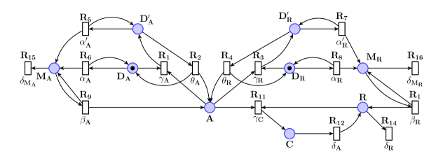
Figure 9: GSPN encoding of the system (2) of chemical equations corresponding to the circadian-clock.

Figure 10: Single trajectory showing the oscillatory character of activator $A$ and repressor $B$ dynamics with normal repressor’s degradation rate $\delta_{R}\!=\!0.2$ (left) and with $10\times$ speed-up, i.e. $\delta_{R}=2$ (right).

The model of Figure 8 corresponds to the system of chemical equations (2), whose (continuous) kinetic rates (taken from [26]) are given in Table 3.

Figure 11: The PDF (left) and the mean value vs the fluctuation (right) of the period of oscillations of protein $A$ of the circadian clock measured with ${\cal A}_{period}$ in function of the repressor’s degradation rate.

Stochastic model

Equations (2) can give rise to either a system of ODEs or to a stochastic process. Here we focus on the discrete-stochastic semantics: Figure 9 shows the GSPN encoding of equations (2) developed with C OSMOS . The configuration of the GSPN (i.e. the stochastic process) requires setting the initial population and the rates of each transition (i.e. reaction). For the initial population, following [26], we observe that the model comprises one gene $D_{A}$ and one $D_{R}$, which can either be in free-state (no activator $A$ is attached to the promoter) or in activator-bound state, i.e. $D^{\prime}_{A}$, respectively $D^{\prime}_{R}$. As a consequence the population of species $D_{A}$ and $D_{R}$ is bounded by the following invariant constraints: $D_{A}+D^{\prime}_{A}=1$ and $D_{R}+D^{\prime}_{R}=1$ (in fact places DA, DA’ and DR, DR’ of net in Figure 9 are the only places covered by P-invarriants). The remaining species are initially supposed to be “empty”, hence they are initialised to $0$. Concerning the transition rates, for simplicity we assume a unitary volume of the system under consideration, hence all continuous rates in Table 3 can be used straightforwardly as rates of the corresponding discrete-stochastic reactions. In this case we assume all reactions following a negative exponential law.

The oscillatory dynamics of the GSPN model of Figure 9 can be observed by plotting of a simulated trajectory (Figure 10). Observe that the frequency of oscillations varies considerably with the degradation rate of the repressor ($R$) protein: a faster degradation of $R$ (right), intuitively, results in a higher frequency of oscillations. In the remainder we formally assess the oscillatory characteristics (i.e. the period and the peaks of oscillations) of the circadian clock model by application of the previously described approach, i.e. by analysing the stochastic process deriving from synchronisation of the circadian clock GSPN model with the ${\cal A}_{period}$ and ${\cal A}_{peaks}$ automata.

Measuring the period of the circadian clock.

We performed a number of experiments aimed at assessing the effect that the degradation rate of the repressor protein ($\delta_{R}$) has on the period of the circadian oscillator. Figure 11 (right) shows three plots representing the PDF of the period (obtained through the HASL formula $({\cal A}_{period},PDF(Last(t)/N))$ for three values of $\delta_{R}$. With $\delta_{R}=0.2$ (i.e. the original value as given in [26]) the PDF is centred at $t=24.9$, i.e. slightly more of the standard 24 hours period expected for a circadian clock. On the other hand speeding up the repressor degradation of 10 times (i.e. $\delta_{R}=2$) yields a slightly more than halved oscillation period (i.e. PDF centred at $T=10.8$). Finally slowing down the degradation rate of a half (i.e. $\delta_{R}=0.1$) yields a less than doubled oscillation period (i.e. PDF centred at $T=40.7$).

Figure 12: The mean value of the minimal and maximal peaks of proteins $A$ and $R$ of the circadian clock measured with ${\cal A}_{peaks}$ in function of the repressor’s degradation rate.

Figure 11 (left) shows plots for the period mean value (red plot) and the period fluctuation (blue plot, as described in Section 3.1) in function of the degradation rate $\delta_{R}$. They indicate that slowing down the degradation of the repressor yields, on one hand, to a lower the frequency of oscillations, and on the other, augmenting the irregularity of the periods (i.e. augmenting the period’s fluctuations). All plots in Figure 11 result from sampling of finite trajectories consisting of $N\!=\!100$ periods, where periods have been detected using $L\!=\!1$ and $H\!=\!1000$ as partition thresholds, and target estimates have been computed with confidence level 99 and confidence-interval width of 0.01. Furthermore the PDF plots in Figure 11 (right) have been computed using a discretisation of the period support interval $[0,50]$ into subintervals of width 0.1.

Measuring the peaks of oscillations of the circadian clock.

We performed a number of experiments aimed at assessing the effect that the degradation rate of the repressor protein ($\delta_{R}$) has on the peaks of oscillation for both protein $A$ and $R$. Figure 12 shows plots for the mean value of the minimal and maximal peaks of oscillations for both $A$ and $R$. Results indicate that while the degradation rate $\delta_{R}$ has no effect on the oscillation peaks of $A$ (both maximal and minimal peaks of $A$ are constant independently of $\delta_{R}$), it affects the maximal peaks (only) of $R$. Specifically the mean value of $R$’s maximal peaks decreases with the increasing of $\delta_{R}$ (while the minimal peaks of $R$ are constantly at $0$), notice that this is in agreement with what indicated by the single trajectories depicted in Figure 10. Notice that Figure 12 contains also plot for the absolute maximum of population of $A$ and $R$ measured along the sampled trajectories through trivial HASL expressions $Z\equiv AVG(max(x))$ (where $x$ is a variable used to record the population of the observed species along a synchronising path). All plots in Figure 12 result from sampling of finite trajectories containing of $N\!=\!100$ maximal peaks and using a noise parameter $\delta\!=\!10\%AVG(max(x))$, meaning that for evaluating the mean value of maximal peaks we discarded all critical points distanced one another less than 10% of the absolute maximum of the observed species. Finally, again points of every plot in Figure 12 have been computed with confidence level 99 and confidence-interval width of 0.01.

On the initial transient.

To assess the effect that the initial transient of the circadian clock model have on the period and peaks estimates we repeated all of the above discussed experiments with different values of the $initT$ parameter (e.g. $initT\!\in\!\{10,50,100,500,1000,\ldots\}$) which determines the starting measuring point for ${\cal A}_{period}$ and of ${\cal A}_{peaks}$. The outcomes of repeated experiments turned out to be independent of the chosen $initT$ value, indicating that circadian clock reaches its steady state very quickly.

5 Related work and discussion

The HASL based methodology presented in this paper is by no means the only approach aimed at the analysis of discrete-state stochastic oscillators. In the following we provide a brief (non exhaustive) overview of similar approaches.

Mathematical approaches

The analysis of periodic signals can be achieved through well established signal processing techniques such as, for example, Fast Fourier Transform (FFT) and autocorrelation. Both methods estimate the dominant frequency of a periodic signal given in terms of a sequence of (real-valued) points. In the context of stochastic modelling both FFT and autocorrelation analysis is performed over trajectories generated by a stochastic simulator. In order to increase the accuracy of the estimates usually frequency estimation is then replicated over $N$ trajectories, the final result being given as the average of the frequency estimate of each trajectory (see e.g. [12, 16]). The main appeal of signal processing techniques is due to their simplicity. However, in the context of statistical model checking, adding an (automatic) control on the accuracy of the resulting estimate would require their integration within a confidence interval estimation procedure, something which at best of our knowledge has not yet been done. From an expressiveness point of view it is worth remarking that FFT and autocorrelation are limited to estimating the (mean value) of the frequency of an oscillator but provides no support for assessing other aspects of oscillator such as the location of the oscillation peaks and the regularity (i.e. the fluctuation) of the period. Finally another interesting contribution belonging to the field of mathematical approaches is presented in [18], where the relationship between stochastic oscillators and their continuous-deterministic counterpart is analysed.

Model checking based approaches.

Analysis of oscillators through stochastic model checking techniques has been considered in several works. Application of CSL [5] to the characterisation CTMC biochemical oscillators has been considered, with limited success in [8], and more comprehensively in [24, 25]. In [24] Spieler demonstrated that deciding whether a given CTMC model oscillates sustainably boils down to a steady-state analysis problem where the allegedly oscillating CTMC is coupled with a period detector automata (through manual hard-wiring). In this case the probability that the period of oscillation has a certain value is computed through dedicated CSL steady-state formulae and has been demonstrated through examples on the P RISM  model-checker.

In a recent work measuring of oscillations has been considered with other statistical model checking tools (UPPAAL-SMC and PLASMA) by application of the MITL logic [12]. In this case the analysis of period duration is achieved by detection of a single period of oscillation through nested time-bounded Until formulae.

6 Conclusion

We have presented a methodology for the formal analysis of stochastic models exhibiting an oscillatory behaviour. Such methodology relies on the application of the HASL formalism, a statistical model checking framework suitable for expressing sophisticated performance measures. We have shown how by means of HASL one can define specific LHA automata targeted to the analysis of particular aspects of the dynamics of oscillatory trajectories, such as: the detection of the period and of the peaks of a stochastic oscillator. For the period we have introduced a class of LHA, denoted ${\cal A}_{per}$, for estimating the PDF, the mean value as well as the the fluctuation of the period duration (the latter being an interesting measure related to the regularity of an oscillator frequency). Concerning the peaks we have introduced a class of LHA, ${\cal A}_{peaks}$, for measuring the mean value of the maximal/minimal peaks of oscillation. We have demonstrated the effectiveness of the methodology by studying a well established model of biological oscillator, namely the circadian clock.

References

- [1] Cosmos home page. http://www.lsv.ens-cachan.fr/software/cosmos/.
- [2] M. Ajmone Marsan, G. Balbo, G. Conte, S. Donatelli, and G. Franceschinis. Modelling with Generalized Stochastic Petri Nets. John Wiley & Sons, 1995.
- [3] R. Alur, C. Courcoubetis, and D. Dill. Model-checking for probabilistic real-time systems. In ICALP’91, LNCS 510, 1991.
- [4] O. Andrei and M. Calder. Trend-based analysis of a population model of the akap scaffold protein. T. Comp. Sys. Biology, 14:1–25, 2012.
- [5] C. Baier, B. Haverkort, H. Hermanns, and J.-P. Katoen. Model-checking algorithms for CTMCs. IEEE Trans. on Software Eng., 29(6), 2003.
- [6] P. Ballarini, H. Djafri, M. Duflot, S. Haddad, and N. Pekergin. COSMOS: A statistical model checker for the hybrid automata stochastic logic. In Proceedings of the 8th International Conference on Quantitative Evaluation of Systems (QEST’11), pages 143–144. IEEE Computer Society Press, sep. 2011.
- [7] P. Ballarini, H. Djafri, M. Duflot, S. Haddad, and N. Pekergin. HASL: an expressive language for statistical verification of stochastic models. In Proc. Valuetools, 2011.
- [8] P. Ballarini and M. Guerriero. Query-based verification of qualitative trends and oscillations in biochemical systems. Theoretical Computer Science, 411(20):2019 – 2036, 2010.
- [9] P. E. Bulychev, A. David, K. G. Larsen, M. Mikucionis, D. B. Poulsen, A. Legay, and Z. Wang. Uppaal-smc: Statistical model checking for priced timed automata. In Proceedings 10th Workshop on Quantitative Aspects of Programming Languages and Systems, volume 85 of EPTCS, pages 1–16, 2012.
- [10] T. Chen, T. Han, J.-P. Katoen, and A. Mereacre. Quantitative model checking of CTMC against timed automata specifications. In Proc. LICS’09, 2009.
- [11] CosyVerif home page. http://www.cosyverif.org.
- [12] A. David, K. G. Larsen, A. Legay, M. Mikucionis, D. B. Poulsen, and S. Sedwards. Runtime verification of biological systems. In ISoLA (1), pages 388–404, 2012.
- [13] S. Donatelli, S. Haddad, and J. Sproston. Model checking timed and stochastic properties with . IEEE Trans. on Software Eng., 35, 2009.
- [14] P. W. Glynn. On the role of generalized semi-Markov processes in simulation output analysis. In Proc. Conf. Winter simulation, 1983.
- [15] T. Herault, R. Lassaigne, and S. Peyronnet. APMC 3.0: Approximate verification of discrete and continuous time Markov chains. In Proc. QEST’06, 2006.
- [16] A. Ihekwaba and S. Sedwards. Communicating oscillatory networks: frequency domain analysis. BMC Systems Biology, 5(1):203, 2011.
- [17] C. Jégourel, A. Legay, and S. Sedwards. A platform for high performance statistical model checking - plasma. In TACAS, volume 7214 of Lecture Notes in Computer Science, pages 498–503, 2012.
- [18] J. Júlvez, M. Kwiatkowska, G. Norman, and D. Parker. Evaluation of sustained stochastic oscillations by means of a system of differential equations. International Journal of Computers and Applications (IJCA), 19(2):101–111, 2012.
- [19] J. P. Katoen and I. S. Zapreev. Simulation-based CTMC model checking: an empirical evaluation. In Proc. QEST’09, 2009.
- [20] D. E. Knuth. The Art of Computer Programming, Volume 2 (3rd Ed.): Seminumerical Algorithms. Addison-Wesley Longman Publishing Co., Inc., Boston, MA, USA, 1997.
- [21] M. Kwiatkowska, G. Norman, and D. Parker. Stochastic model checking. In Formal Methods for the Design of Computer, Communication and Software Systems: Performance Evaluation, volume 4486 of LNCS, pages 220–270. Springer, 2007.
- [22] Prism home page. http://www.prismmodelchecker.org.
- [23] K. Sen, M. Viswanathan, and G. Agha. VESTA: A statistical model-checker and analyzer for probabilistic systems. In Proc. QEST’05, 2005.
- [24] D. Spieler. Model checking of oscillatory and noisy periodic behavior in markovian population models. Master’s thesis, Saarland University, 2009.
- [25] D. Spieler. Characterizing oscillatory and noisy periodic behavior in markov population models. In Proc. QEST’13, 2013.
- [26] J. Vilar, H.-Y. Kueh, N. Barkai, and S. Leibler. Mechanisms of noise-resistance in genetic oscillators. Proc. National Academy of Sciences of the United States of America, 99(9):5988–5992, 2002.
- [27] H. L. Younes. Ymer: A statistical model checker. In Computer Aided Verification, pages 429–433. Springer, 2005.