Radiative energy and momentum transfer for various spherical shapes: a single sphere, a bubble, a spherical shell and a coated sphere

Abstract

We use fluctuational electrodynamics to determine emissivity and van der Waals contribution to surface energy for various spherical shapes, such as a sphere, a bubble, a spherical shell and a coated sphere, in a homogeneous and isotropic medium. Near-field radiative transfer and momentum transfer between flat plates and curved surfaces have been studied for the past decades, however the investigation of radiative heat transfer and van der Waals stress due to fluctuations of electromagnetic fields for a single object is missing from literature. The dyadic Green’s function formalism of radiative energy and fluctuation-induced van der Waals stress for different spherical configurations have been developed. We show (1) emission spectra of micro and nano-sized spheres display several emissivity sharp peaks as the size of object reduces, and (2) surface energy becomes size dependent due to van der Waals phenomena when size of object is reduced to a nanoscopic length scale.

I Introduction

Quantum and thermal fluctuations of electromagnetic fields, which give rise to Planck’s law of blackbody radiation Planck (2011), are responsible for radiative energy, momentum and entropy transfer Zheng (2014); Basu et al. (2009); Zheng and Narayanaswamy (2014a); Francoeur et al. (2011); Narayanaswamy and Zheng (2013a). Classical theory of thermal radiation takes only propagating waves into consideration Planck (2011). Presence of evanescent waves nearby the surfaces leads to near-field effects, such as interference, diffraction and tunneling of surface waves, which are important when the size and length scale is comparable to the thermal wavelength of objects ($\approx$ 10 $\mu$m at room temperature 300 K) Zheng (2014). Enhancement of radiative energy transfer, wavelength selectivity, and size and scale dependence are typical characteristics of near-field phenomena which make it more interesting. These characteristics could be exploited in many potential nanotechnological applications such as nanoparticles Pérez-Madrid et al. (2008); Huth et al. (2010); Von Werne and Patten (1999); Biehs and Greffet (2010) and wavelength selective absorber and emitters Rephaeli and Fan (2009); Avitzour et al. (2009); Sergeant et al. (2010); Cao et al. (2010); Narayanaswamy et al. (2014). Fluctuations in electromagnetic fields due to the presence of boundaries create van der Waals pressures which lead to momentum transfer Belosludov and Nabutovskiy (1975); Pitaevskii (2006); Narayanaswamy and Zheng (2013b); Parsegian (2006). These phenomena can be described by cross-spectral densities of the electromagnetic field using dyadic Green’s functions of vector Helmholtz equation Tai (1994); Narayanaswamy and Zheng (2014); Yla-Oijala and Taskinen (2003). Such a relation between near-field radiative energy and momentum transfer for arbitrarily shaped objects has been explicitly derived in Ref. Narayanaswamy and Zheng (2014).

During the past decades, many theoretical works have been published on the topic of the enhanced thermal radiation due to near-field effects and fluctuation-induced van der Waals pressures. Most of them are focused on the configurations, for example, between planar multilayered media Ottens et al. (2011); Francoeur et al. (2009); Dzyaloshinskii et al. (1961); Narayanaswamy and Zheng (2013b); Parsegian and Ninham (1973); Antezza et al. (2008), cylindrical objects Sheikholeslami and Ganji (2014); Edalatpour and Francoeur (2014), spheres Pérez-Madrid et al. (2008); Sasihithlu and Narayanaswamy (2011); Zhu et al. (2013); Narayanaswamy et al. (2008); Incardone et al. (2014), and a sphere and a flat plate Otey and Fan (2011); Biehs and Greffet (2010); Otey et al. (2014); Incardone et al. (2014). Although considerable amount of work devoted to theoretical and experimental results for near-field radiative energy transfer and momentum transfer between objects of the abovementioned typical geometries, these phenomena for a single object have not been studied well to the best of our knowledge. In this paper, emissivity of thermal radiation and van der Waals contribution to surface energy are determined for micro and nano-sized spherical objects of interest, such as a single sphere, a bubble, a sherical shell and a coated sphere, as shown in Fig. 1.

This paper demonstrates how fluctuational electrodynamics can be used to determine emissivity and van der Waals contribution to surface energy for various shapes in a homogenous and isotropic medium. The dyadic Green’s function formalism of radiative heat transfer and van der Waals stress for different spherical configurations has been developed. Size dependence and wavelength selectivity of micro and nano-sized spheres are clearly observed. For small sized objects, the emissivity spectra show sharp peaks at wavelengths corresponding to characteristics of the material’s refractive index. The peaks increase as size of object decreases. This is consistent with emissivity calculations done for thin film as in Ref. Narayanaswamy et al. (2014). The calculations for a spherical bubble show that as radius of the bubble reduces, van der Waals energy contribution to the total surface energy increases and dominates it beyond a critical value.

The paper is arranged as follows. Section II focuses on the theoretical formulations for near-field radiative energy transfer and momentum transfer for a generalized case. Calculations of transmissivity for radiative energy transfer and fluctuation-induced van der Waals pressure are discussed in Sec. II.1 and Sec. II.2, respectively. Using this formalism, the analytical expressions of Mie reflection and transmission coefficients for specific cases of a sphere, a bubble, a spherical shell and a coated sphere in a homogeneous and isotropic medium are obtained in Sec. III. Formulae for calculations of emissivity and van der Waals contribution to surface energy of a spherical body are subsequently derived in Sec. III.1 and Sec. III.2. We recapitulate the paper and states the conclusions in Sec. IV.

Figure 1: Schematic of various spherical geometries. (a) a sphere of radius $r$ (material 1, green), (b) a bubble of radius $r$ in material 2 (blue), (c) a spherical shell of interior and exterior radii $r_{1}$ and $r_{2}$ (material 2, orange), and (d) a sphere of radius $r_{1}$ (material 1, green) coated with a thin film of thickness $r_{2}-r_{1}$ (material 2, orange) in material 3 (blue). The short arrows on either side of the interface between two materials denote the spherical electromagnetic waves $U$($\bm{M}$ and $\bm{N}$ waves). $U_{lm}^{(p)}$ is vector spherical wave functions of order $(l,m)$, and superscript $(p)$ refers to the radial behavior of the waves. $k_{i}$ is wavenumber in medium $i$, $R_{ij,l}^{(U)}$ and $T_{ij}^{(U)}$ are the Mie reflection and transmission coefficients due to spherical electromagnetic waves $U$ from medium $i$ to medium $j$, respectively.

II Theoretical fundamentals

The Fourier transforms of the electric and magnetic fields due to thermal sources in any object (volume $V_{s}$) are given by Rytov (1967); Narayanaswamy and Zheng (2014)

$$\mathbf{E}(\mathbf{\tilde{r}})=\int\limits_{V_{s}}[\mathbf{p}(\mathbf{r})\cdot\overline{\overline{\mathbf{G}}}_{e}(\mathbf{r},\mathbf{\tilde{r}})-\mathbf{J}^{m}(\mathbf{r})\cdot\overline{\overline{\mathbf{G}}}_{E}(\mathbf{r},\mathbf{\tilde{r}})]d\mathbf{r}$$ (1a)

$$\mathbf{H}(\mathbf{\tilde{r}})=\int\limits_{V_{s}}[\mathbf{m}(\mathbf{r})\cdot\overline{\overline{\mathbf{G}}}_{m}(\mathbf{r},\mathbf{\tilde{r}})+\mathbf{J}^{e}(\mathbf{r})\cdot\overline{\overline{\mathbf{G}}}_{M}(\mathbf{r},\mathbf{\tilde{r}})]d\mathbf{r}$$ (1b)

where source position vector $\mathbf{r}\in V_{s}$, observation position vector $\mathbf{\tilde{r}}$, $\mathbf{J}^{e}$ and $\mathbf{J}^{m}$ are the electric and magnetic current densities, $\mathbf{p}\left(\mathbf{r}\right)$$=$$i\omega\mu_{o}\mu(\mathbf{r})\mathbf{J^{e}}\left(\mathbf{r}\right)$, $\mathbf{m}\left(\mathbf{r}\right)=i\omega\varepsilon_{o}\varepsilon(\mathbf{r})\mathbf{J^{m}}\left(\mathbf{r}\right)$, $\varepsilon_{o}$ and $\mu_{o}$ are the permittivity and permeability of free space, and, $\varepsilon(\mathbf{r})$ and $\mu(\mathbf{r})$ are the permittivity and permeability at location $\mathbf{r}$. $\overline{\overline{\mathbf{G}}}_{E}(\mathbf{r},\mathbf{\tilde{r}})=\nabla\times\overline{\overline{\mathbf{G}}}_{e}(\mathbf{r},\mathbf{\tilde{r}})$ and $\overline{\overline{\mathbf{G}}}_{M}(\mathbf{r},\mathbf{\tilde{r}})=\nabla\times\overline{\overline{\mathbf{G}}}_{m}(\mathbf{r},\mathbf{\tilde{r}})$. $\overline{\overline{\mathbf{G}}}_{e}(\mathbf{r},\mathbf{\tilde{r}})$ and $\overline{\overline{\mathbf{G}}}_{m}(\mathbf{r},\mathbf{\tilde{r}})$ are dyadic Green’s functions of the vector Helmholtz equation that satisfy the following boundary conditions on the interface between object 1 and object 2. For electric dyadic Green’s functions,

$$\hat{\mathbf{n}}_{1}\times\mu_{1}\overline{\overline{\mathbf{G}}}_{e}(\mathbf{r}_{1},\mathbf{\tilde{r}})=\hat{\mathbf{n}}_{2}\times\mu_{2}\overline{\overline{\mathbf{G}}}_{e}(\mathbf{r}_{2},\mathbf{\tilde{r}}),$$ (2a)

$$\hat{\mathbf{n}}_{1}\times\overline{\overline{\mathbf{G}}}_{E}(\mathbf{r}_{1},\mathbf{\tilde{r}})=\hat{\mathbf{n}}_{2}\times\overline{\overline{\mathbf{G}}}_{E}(\mathbf{r}_{2},\mathbf{\tilde{r}}),$$ (2b)

and for magnetic dyadic Green’s functions,

$$\hat{\mathbf{n}}_{1}\times\varepsilon_{1}\overline{\overline{\mathbf{G}}}_{m}(\mathbf{r}_{1},\mathbf{\tilde{r}})=\hat{\mathbf{n}}_{2}\times\varepsilon_{2}\overline{\overline{\mathbf{G}}}_{m}(\mathbf{r}_{2},\mathbf{\tilde{r}}),$$ (2c)

$$\hat{\mathbf{n}}_{1}\times\overline{\overline{\mathbf{G}}}_{M}(\mathbf{r}_{1},\mathbf{\tilde{r}})=\hat{\mathbf{n}}_{2}\times\overline{\overline{\mathbf{G}}}_{M}(\mathbf{r}_{2},\mathbf{\tilde{r}}),$$ (2d)

where $\hat{\mathbf{n}}_{1}$ and $\hat{\mathbf{n}}_{2}$ are surface normal vectors, and $\mathbf{r}_{1}$ and $\mathbf{r}_{2}$ are position vectors of points on either side of interface in volume $V_{1}$ and $V_{2}$, as $\lvert\mathbf{r}_{1}-\mathbf{r}_{2}\rvert\rightarrow 0$.

II.1 Transmissivity for radiative energy transfer

The steady state radiative heat transfer from object $1$ to object $2$, $\mathcal{Q}_{1\rightarrow 2}$, is given by

$$\mathcal{Q}_{1\rightarrow 2}=-\oint\limits_{S_{2}}\mathbf{P}(\mathbf{\tilde{r}})\cdot\hat{\mathbf{n}}_{2}d\mathbf{\tilde{r}}$$ (3)

where $\mathbf{P}(\mathbf{\tilde{r}})=\langle\mathbf{E}(\mathbf{\tilde{r}},t)\times\mathbf{H}(\mathbf{\tilde{r}},t)\rangle$ is the Poynting vector at $\mathbf{\tilde{r}}\in S_{2}$ due to thermally fluctuating sources within $V_{1}$. $\langle$ $\rangle$ denotes the ensemble average, and the “$-$” sign in front of the surface integral is because $\hat{\mathbf{n}}_{2}$ is the outward pointing normal on the surface $S_{2}$. The components of $\mathbf{P}(\mathbf{\tilde{r}})$ are given by

$$P_{i}(\mathbf{\tilde{r}})=\epsilon_{ipq}\langle E_{p}(\mathbf{\tilde{r}},t)H_{q}(\mathbf{\tilde{r}},t)\rangle$$ (4)

where $p$, $q$=1,2,3 are the labels for the Cartesian components of the vector, $\epsilon_{ipq}$ is the Levi-Civita symbol, $\langle E_{p}(\mathbf{\tilde{r}},t)H_{q}(\mathbf{\tilde{r}},t)\rangle$ is the contribution to $\langle E_{p}(\mathbf{\tilde{r}},t)H_{q}(\mathbf{\tilde{r}},t)\rangle$ from sources within $V_{1}$. We note that $\displaystyle\langle E_{q}(\mathbf{\tilde{r}},t)H_{p}(\mathbf{\tilde{r}},t)\rangle=\int\limits_{0}^{\infty}\frac{d\omega}{2\pi}\langle E_{q}(\mathbf{\tilde{r}},\omega)H_{p}^{*}(\mathbf{\tilde{r}},\omega)\rangle$. Using Eq. 1a and Eq. 1b, Eq. 3 for $\mathcal{Q}_{1\rightarrow 2}$ can be re-written as

$$\begin{split}\mathcal{Q}_{1\rightarrow 2}=\int\limits_{0}^{\infty}d\omega\frac{\hbar\omega}{2\pi}\coth\left(\frac{\hbar\omega}{2k_{B}T_{1}}\right)\mathcal{T}_{rr}(\omega)\end{split}$$ (5)

where $k_{B}$ is Boltzmann constant, $2\pi\hbar$ is the Planck constant, $T_{1}$ is the absolute temperature of object 1, and $\mathcal{T}_{rr}(\omega)$ is a generalized transmissivity for radiative energy transport between objects 1 and 2. $\mathcal{T}_{rr}(\omega)$ can be expressed exclusively in terms of components of the dyadic Green’s functions on the surfaces of objects 1 and 2, which is given by Narayanaswamy and Zheng (2014)

$$\begin{split}\mathcal{T}_{rr}(\omega)=\Re Tr\oint\limits_{S_{1}}d\mathbf{r}\oint\limits_{S_{2}}d\mathbf{\tilde{r}}\bigg{[}\frac{\omega^{2}}{c^{2}}\left[\mathbf{\hat{n}}_{2}\times\mu_{2}\overline{\overline{G}}_{e}(\mathbf{\tilde{r}},\mathbf{r})\right]\cdot\left[\mathbf{\hat{n}}_{1}\times\varepsilon_{1}^{*}\overline{\overline{G}}_{m}^{*}(\mathbf{r},\mathbf{\tilde{r}})\right]+\left[\mathbf{\hat{n}}_{2}\times\overline{\overline{G}}_{E}(\mathbf{\tilde{r}},\mathbf{r})\right]\cdot\left[\mathbf{\hat{n}}_{1}\times\overline{\overline{G}}^{*}_{E}(\mathbf{r},\mathbf{\tilde{r}})\right]\bigg{]}\end{split}$$ (6)

where $\Re$ stands for the real part, superscript ^∗ denotes the complex conjugate, and operator trace $Tr(\overline{\overline{A}})=\sum\limits_{p=1}^{3}A_{pp}$.

II.2 van der Waals stress for radiative momentum transfer

Radiative momentum transfer arose from the fluctuations of electromagnetic fields is responsible for the van der Waals pressure, which can be determined from the electromagnetic stress tensor, $\overline{\overline{\sigma}}=\overline{\overline{\sigma}}_{e}+\overline{\overline{\sigma}}_{m}$, where $\overline{\overline{\sigma}}_{e}$ and $\overline{\overline{\sigma}}_{m}$ are the electric and magnetic field contributions respectively. Stress tensors $\overline{\overline{\sigma}}_{e}$ and $\overline{\overline{\sigma}}_{m}$ are given by Zheng and Narayanaswamy (2011); Narayanaswamy and Zheng (2013b)

$$\overline{\overline{\sigma}}_{e}(\mathbf{\tilde{r}})=\varepsilon_{o}\left[\langle\mathbf{E}(\mathbf{\tilde{r}},t)\mathbf{E}(\mathbf{\tilde{r}},t)\rangle-\frac{1}{2}\overline{\overline{I}}\langle\mathbf{E}^{2}(\mathbf{\tilde{r}},t)\rangle\right]$$ (7a)

$$\overline{\overline{\sigma}}_{m}(\mathbf{\tilde{r}})=\mu_{o}\left[\langle\mathbf{H}(\mathbf{\tilde{r}},t)\mathbf{H}(\mathbf{\tilde{r}},t)\rangle-\frac{1}{2}\overline{\overline{I}}\langle\mathbf{H}^{2}(\mathbf{\tilde{r}},t)\rangle\right],$$ (7b)

where $\overline{\overline{I}}$ is the identity matrix, $\langle\mathbf{E}(\mathbf{\tilde{r}},t)\mathbf{E}(\mathbf{\tilde{r}},t)\rangle$ and $\langle\mathbf{H}(\mathbf{\tilde{r}},t)\mathbf{H}(\mathbf{\tilde{r}},t)\rangle$ are matrices whose components are $\langle E_{p}(\mathbf{\tilde{r}},t)E_{q}(\mathbf{\tilde{r}},t)\rangle$ and $\langle H_{p}(\mathbf{\tilde{r}},t)H_{q}(\mathbf{\tilde{r}},t)\rangle$ respectively.

Relying on Rytov’s theory of fluctuational electrodynamics Rytov (1967), the cross-spectral correlations of the electric and magnetic field components can be written as Narayanaswamy and Zheng (2014)

$$\begin{split}\left<E_{i}(\mathbf{\tilde{r}},\omega)E_{j}^{*}(\mathbf{\tilde{r}},\omega)\right>=&\frac{\hbar\omega^{2}}{\pi}\mu_{0}\coth\left(\frac{\hbar\omega}{2k_{B}T}\right)\\ &\times\Im\left[\varepsilon(\omega)\mu(\omega)G_{e,ij}(\mathbf{\tilde{r}},\mathbf{\tilde{r}})\right]\end{split}$$ (8a)

$$\begin{split}\left<H_{i}(\mathbf{\tilde{r}},\omega)H_{j}^{*}(\mathbf{\tilde{r}},\omega)\right>=&\frac{\hbar\omega^{2}}{\pi}\varepsilon_{0}\coth\left(\frac{\hbar\omega}{2k_{B}T}\right)\\ &\times\Im\left[\varepsilon(\omega)\mu(\omega)G_{m,ij}(\mathbf{\tilde{r}},\mathbf{\tilde{r}})\right]\end{split}$$ (8b)

where $\Im$ denotes the imaginary part. $\varepsilon(\omega)$ and $\mu(\omega)$ are frequency dependent permittivity and permeability of region in which $\mathbf{\tilde{r}}$ is located. $\sqrt{\varepsilon(\omega)}=n(\omega)+i\kappa(\omega)$ and $\mu(\omega)=1$. The optical data for $n$ and $\kappa$ can be obtained from Refs. Hough and White (1980); Palik (1998). The van der Waals pressure on the interior surface of a bubble or the exterior surface of a sphere of radius $r$ in an otherwise homogeneous medium (see Figs. 1a and 1b) can be obtained from the $\hat{r}\hat{r}$ component of the electromagnetic stress tensor, in terms of dyadic Green’s functions, which is given by

$$\begin{split}\mathcal{S}_{rr}(r)&=\int\limits_{0}^{\infty}d\omega\frac{\hbar\omega^{2}}{\pi c^{2}}\coth\!\left(\!\frac{\hbar\omega}{2k_{B}T}\!\right)\Im\Bigg{\{}\varepsilon(\omega)\mu(\omega)\left[G_{e,\hat{r}\hat{r}}(\bm{r},\bm{r})-\frac{1}{2}Tr\overline{\overline{G}}_{e}(\bm{r},\bm{r})+G_{m,\hat{r}\hat{r}}(\bm{r},\bm{r})-\frac{1}{2}Tr\overline{\overline{G}}_{m}(\bm{r},\bm{r})\right]\!\Bigg{\}}\end{split}$$ (9)

where $Tr$ is the trace of the tensor in the spherical coordinates, that is $Tr\left(\overline{\overline{G}}_{p}\right)=G_{p,\hat{r}\hat{r}}+G_{p,\hat{\theta}\hat{\theta}}+G_{p,\hat{\phi}\hat{\phi}}$. The integral on the right hand side of Eq. 9 is of the form $\int\limits_{0^{+}}^{\infty}d\omega\coth\left(\frac{\hbar\omega}{2k_{B}T_{l}}\right)\Im f(\omega)$, in which the function $f(\omega+i\xi)$ is analytic in the upper–half of the complex plane ($\xi>0$). Since $\displaystyle G\left(\bm{r},\omega\right)$ is analytic in the upper–half of the complex plane, the integral along the real frequency axis can be transformed into summation over Matsubara frequencies, $i\xi_{n}=in2\pi k_{B}T_{l}/\hbar$, as $\displaystyle-\frac{2\pi k_{B}T}{\hbar}\sum\limits_{n=0}^{\infty}\phantom{}{}^{{}^{\prime}}f(i\xi_{n})$. $\sum\limits_{n=0}^{\infty}\phantom{}{}^{{}^{\prime}}$ indicates that the $n=0$ term is multiplied by 1/2 Lifshitz (1956).

$\mathcal{S}_{p}\left(r\right)$ can be split into two parts: (1) a part which arises from the dyadic Green’s function in an infinite homogeneous medium, and (2) a part which arises from the scattered dyadic Green’s function due to the presence of boundaries, as $\mathcal{S}_{p}\left(r\right)=\mathcal{S}^{(o)}\left(r\right)+\mathcal{S}_{p}^{(sc)}\left(r\right)$. Since $\mathcal{S}^{(o)}\left(r\right)$ is the stress tensor contribution from the homogeneous medium, there is no distinction between the $p=e$ or $p=m$ contributions. The homogeneous part of dyadic Green’s function ($\overline{\overline{G}}_{e}^{(o)}(\mathbf{r},\mathbf{\tilde{r}})$) on either side of the interface between objects 1 and 2 (as shown in Fig. 1) cancels out, while the scattered part of dyadic Green’s function is important, which leads to the dispersion force due to the scattering of fluctuations of electromagnetic fields.

The expressions for $\overline{\overline{G}}_{e}^{(sc)}(\mathbf{r},\mathbf{\tilde{r}})$ when $\mathbf{r},\mathbf{\tilde{r}}\in V_{2}$ (Fig. 1a) and $\mathbf{r},\mathbf{\tilde{r}}\in V_{1}$ (Fig. 1b), respectively, are given by

$$\begin{split}\overline{\overline{G}}_{e}&{}^{(sc)}(\bm{r},\bm{\tilde{r}})=ik_{2}\sum\limits_{m=-l,\atop l=0}^{l=\infty,\atop m=l}(-1)^{m}\\ &\times\left[\begin{array}[]{l}R_{22,l}^{(M)}\bm{M}_{l,m}^{(3)}\left(k_{2}\bm{r}\right)\bm{M}_{l,-m}^{(3)}\left(k_{2}\bm{\tilde{r}}\right)+\\ R_{22,l}^{(N)}\bm{N}_{l,m}^{(3)}\left(k_{2}\bm{r}\right)\bm{N}_{l,-m}^{(3)}\left(k_{2}\bm{\tilde{r}}\right)\end{array}\right]\end{split}$$ (10a)

$$\begin{split}\overline{\overline{G}}_{e}&{}^{(sc)}(\bm{r},\bm{\tilde{r}})=ik_{1}\sum\limits_{m=-l,\atop l=0}^{l=\infty,\atop m=l}(-1)^{m}\\ &\times\left[\begin{array}[]{l}R_{11,l}^{(M)}\bm{M}_{l,m}^{(1)}\left(k_{1}\bm{r}\right)\bm{M}_{l,-m}^{(1)}\left(k_{1}\bm{\tilde{r}}\right)+\\ R_{11,l}^{(N)}\bm{N}_{l,m}^{(1)}\left(k_{1}\bm{r}\right)\bm{N}_{l,-m}^{(1)}\left(k_{1}\bm{\tilde{r}}\right)\end{array}\right]\end{split}$$ (10b)

where, $R_{ij,l}^{(U)}$ is the Mie refection coefficient due to the source in region $i$ to the observation in region $j$ due to $U=\bm{M,N}$ waves. When $|\bm{r}|>|\bm{\tilde{r}}|$. $k_{i}=\omega\sqrt{\varepsilon_{i}(\omega)\mu_{i}(\omega)}/c$ is the wavenumber in region $i$ ($i=1,2,3$), $\bm{M}_{l,m}^{(p)}(k_{i}r)$ and $\bm{N}_{l,m}^{(p)}(k_{i}r)$ are vector spherical wave functions of order $(l,m)$, and superscript $(p)$ refers to the radial behavior of the waves, given by Narayanaswamy and Chen (2008)

$$\bm{M}_{l,m}^{(p)}(k_{i}r)=\frac{z_{l}^{(p)}(k_{i}r)}{\sqrt{l(l+1)}}\left(\hat{\theta}\frac{imY_{l,m}}{\sin\theta}-\hat{\phi}\frac{\partial Y_{l,m}}{\partial\theta}\right)$$ (11a)

$$\begin{split}\bm{N}_{l,m}^{(p)}(k_{i}r)=&\hat{r}\frac{z_{l}^{(p)}(k_{i}r)}{k_{i}r}\sqrt{l(l+1)}Y_{l,m}\\ &+\frac{\xi_{l}^{(p)}(k_{i}r)}{\sqrt{l(l+1)}}\left(\hat{\theta}\frac{\partial Y_{l,m}}{\partial\theta}+\hat{\phi}\frac{imY_{l,m}}{\sin\theta}\right)\end{split}$$

For superscript $p=1$, both $\bm{M}$ and $\bm{N}$ waves are regular vector spherical waves and $z_{l}^{(1)}$ is the spherical Bessel function of first kind of order $l$. For superscript $p=3$, both $\bm{M}$ and $\bm{N}$ waves are outgoing spherical waves and $z_{l}^{(3)}$ is the spherical Hankel function of first kind of order $l$. $\xi_{l}^{(p)}$ is first derivative of Bessel (Hankel) function, defined as $x\xi_{l}^{(p)}(x)=\displaystyle\frac{d}{dx}\left[xz_{l}^{(p)}(x)\right]$. $Y_{l,m}$ is the spherical harmonic of order $(l,m)$.

III Results and Discussion

The spherical configurations of interest in this paper are shown in Fig. 1. To determine the generalized transmissivity for radiative energy transport (Eq. 6) and van der Waals stress (Eq. 9) for these geometries, we need to find the corresponding electric and/or magnetic dyadic Green’s functions, which are expressed in terms of the Mie reflection coefficients. Here, we list boundary conditions of electromagnetic fields to be used to calculate the Mie reflection and transmission coefficients for the four cases: (a) a sphere of radius $r$, (b) a bubble of radius $r$, (c) a spherical shell of interior and exterior radii $r_{1}$ and $r_{2}$, and (d) a sphere of radius $r_{1}$ with a coating of thickness $r_{2}-r_{1}$ (the same as case (c) in mathematics).

Case (a): A sphere of radius $r$. Radius $r_{+}=r+\delta$ and $\delta\rightarrow 0$. Thermal sources outside the sphere, $r\in V_{2}$. The boundary conditions are given by

$$\begin{cases}\mu_{2}z_{l}^{(1)}(k_{2}r)+R_{22,l}^{(M)}\mu_{2}z_{l}^{(3)}(k_{2}r)=T_{21,l}^{(M)}\mu_{1}z_{l}^{(1)}(k_{1}r)\\ k_{2}\xi_{l}^{(1)}(k_{2}r)+R_{22,l}^{(M)}k_{2}\xi_{l}^{(3)}(k_{2}r)=T_{21,l}^{(M)}k_{1}\xi_{l}^{(1)}(k_{1}r)\end{cases}$$ (12)

Case (b): A bubble of radius $r$. Radius $r_{-}=r-\delta$ and $\delta\rightarrow 0$. Thermal sources inside the bubble, $r\in V_{1}$.

$$\begin{cases}\mu_{1}z_{l}^{(3)}(k_{1}r)+R_{11,l}^{(M)}\mu_{1}z_{l}^{(1)}(k_{1}r)=T_{12,l}^{(M)}\mu_{2}z_{l}^{(3)}(k_{2}r)\\ k_{1}\xi_{l}^{(3)}(k_{1}r)+R_{11,l}^{(M)}k_{1}\xi_{l}^{(1)}(k_{1}r)=T_{12,l}^{(M)}k_{2}\xi_{l}^{(3)}(k_{2}r)\end{cases}$$ (13)

Case (c): A spherical shell of interior radius $r_{1}$ and exterior radius $r_{2}$. (or Case (d): A sphere of radius $r_{1}$ coated with a thin film of thickness $r_{2}-r_{1}$.

Consider thermal sources in material 1, $r\in V_{1}$. At $r=r_{1}$,

$$\begin{cases}\mu_{1}z_{l}^{(3)}(k_{1}r_{1})+{R}_{11,l}^{(M)}\mu_{1}z_{l}^{(1)}(k_{1}r_{1})=\widetilde{R}_{12,l}^{(M)}\mu_{2}z_{l}^{(3)}(k_{2}r_{1})+\widetilde{\widetilde{R}}_{12,l}^{(M)}\mu_{2}z_{l}^{(1)}(k_{2}r_{1})\\ k_{1}\xi_{l}^{(3)}(k_{1}r_{1})+{R}_{11,l}^{(M)}k_{1}\xi_{l}^{(1)}(k_{1}r_{1})=\widetilde{R}_{12,l}^{(M)}k_{2}\xi_{l}^{(3)}(k_{2}r_{1})+\widetilde{\widetilde{R}}_{12,l}^{(M)}k_{2}\xi_{l}^{(1)}(k_{2}r_{1})\end{cases}$$ (14)

and at $r=r_{2}$,

$$\begin{cases}\widetilde{R}_{12,l}^{(M)}\mu_{2}z_{l}^{(3)}(k_{2}r_{2})+\widetilde{\widetilde{R}}_{12,l}^{(M)}\mu_{2}z_{l}^{(1)}(k_{2}r_{2})=T_{23,l}^{(M)}\mu_{3}z_{l}^{(3)}(k_{3}r_{2})\\ \widetilde{R}_{12,l}^{(M)}k_{2}\xi_{l}^{(3)}(k_{2}r_{2})+\widetilde{\widetilde{R}}_{12,l}^{(M)}k_{2}\xi_{l}^{(1)}(k_{2}r_{2})=T_{23,l}^{(M)}k_{3}\xi_{l}^{(3)}(k_{3}r_{2})\end{cases}$$ (15)

And, consider thermal sources in material 3, $r\in V_{3}$. At $r=r_{2}$,

$$\begin{cases}\mu_{3}z_{l}^{(1)}(k_{3}r_{2})+{R}_{33,l}^{(M)}\mu_{3}z_{l}^{(3)}(k_{3}r_{2})=\widetilde{R}_{32,l}^{(M)}\mu_{2}z_{l}^{(1)}(k_{2}r_{2})+\widetilde{\widetilde{R}}_{32,l}^{(M)}\mu_{2}z_{l}^{(3)}(k_{2}r_{2})\\ k_{3}\xi_{l}^{(1)}(k_{3}r_{2})+{R}_{33,l}^{(M)}k_{3}\xi_{l}^{(3)}(k_{3}r_{2})=\widetilde{R}_{32,l}^{(M)}k_{2}\xi_{l}^{(1)}(k_{2}r_{2})+\widetilde{\widetilde{R}}_{32,l}^{(M)}k_{2}\xi_{l}^{(3)}(k_{2}r_{2})\end{cases}$$ (16)

and at $r=r_{1}$,

$$\begin{cases}\widetilde{R}_{32,l}^{(M)}\mu_{2}z_{l}^{(1)}(k_{2}r_{1})+\widetilde{\widetilde{R}}_{32,l}^{(M)}\mu_{2}z_{l}^{(3)}(k_{2}r_{1})=T_{21,l}^{(M)}\mu_{1}z_{l}^{(1)}(k_{1}r_{1})\\ \widetilde{R}_{32,l}^{(M)}k_{2}\xi_{l}^{(1)}(k_{2}r_{1})+\widetilde{\widetilde{R}}_{32,l}^{(M)}k_{2}\xi_{l}^{(3)}(k_{2}r_{1})=T_{21,l}^{(M)}k_{1}\xi_{l}^{(1)}(k_{1}r_{1})\end{cases}$$ (17)

Here, $R_{ij,l}^{(U)}$ and $T_{ij}^{(U)}$ are the Mie reflection and transmission coefficients due to $U$($=\bm{M},\bm{N}$) waves from region $i$ to region $j$, respectively.

For example, the Mie coefficients due to $\bm{M}$ waves $R_{11,l}^{(M)}$ and $T_{12,l}^{(M)}$ in Case (a) can be obtained from Eq. 12 as

$$R_{22,l}^{(M)}=-\frac{\displaystyle\left(\frac{k_{2}}{\mu_{2}}\frac{\xi_{l}^{(1)}(k_{2}a)}{z_{l}^{(1)}(k_{2}r)}-\frac{k_{1}}{\mu_{1}}\frac{\xi_{l}^{(1)}(k_{1}r)}{z_{l}^{(1)}(k_{1}a)}\right)}{\displaystyle\left(\frac{k_{2}}{\mu_{2}}\frac{\xi_{l}^{(3)}(k_{2}a)}{z_{l}^{(3)}(k_{2}r)}-\frac{k_{1}}{\mu_{1}}\frac{\xi_{l}^{(1)}(k_{1}r)}{z_{l}^{(1)}(k_{1}a)}\right)}\frac{z_{l}^{(1)}(k_{2}r)}{z_{l}^{(3)}(k_{2}r)}$$ (18a)

$$T_{21,l}^{(M)}=\frac{\mu_{2}}{\mu_{1}}\left(\frac{y_{l}^{(1)}(k_{2}r)}{y_{l}^{(1)}(k_{1}r)}+R_{22,l}^{(M)}\frac{y_{l}^{(3)}(k_{2}r)}{y_{l}^{(1)}(k_{1}r)}\right)$$ (18b)

and the Mie coefficients due to $\bm{M}$ waves $R_{22,l}^{(M)}$ and $T_{21,l}^{(M)}$ in Case (b) can be obtained from Eq. 13 as

$$R_{11,l}^{(M)}=-\frac{\displaystyle\left(\frac{k_{1}}{\mu_{1}}\frac{\xi_{l}^{(3)}(k_{1}r)}{z_{l}^{(3)}(k_{1}r)}-\frac{k_{2}}{\mu_{2}}\frac{\xi_{l}^{(3)}(k_{2}r)}{z_{l}^{(3)}(k_{2}r)}\right)}{\displaystyle\left(\frac{k_{1}}{\mu_{1}}\frac{\xi_{l}^{(1)}(k_{1}r)}{z_{l}^{(1)}(k_{1}r)}-\frac{k_{2}}{\mu_{2}}\frac{\xi_{l}^{(3)}(k_{2}r)}{z_{l}^{(3)}(k_{2}r)}\right)}\frac{z_{l}^{(3)}(k_{1}r)}{z_{l}^{(1)}(k_{1}r)}$$ (19a)

$$T_{12,l}^{(M)}=\frac{\mu_{1}}{\mu_{2}}\left(\frac{y_{l}^{(3)}(k_{1}r)}{y_{l}^{(3)}(k_{2}r)}+R_{11,l}^{(M)}\frac{y_{l}^{(1)}(k_{1}r)}{y_{l}^{(3)}(k_{2}r)}\right)$$ (19b)

The Mie reflection and transmission coefficients due to $\bm{M}$ waves in Cases (c) and (d) can be obtained by solving Eqs. 14 - 17. Similarly, the Mie coefficients due to $\bm{N}$ waves can be obtained by simply switching functions of $z_{l}$ and $\xi_{l}$ Narayanaswamy and Chen (2008).

III.1 Emissivity of a spherical body

Now, the Mie scattering coefficients and dyadic Green’s functions of a sphere are known. Substituting Eq. 19a, Eq. 19b, Eq. 10a and Eq. 10b into Eq. 6 yields the transmissivity between a single sphere of radius $r$ and a concentric sphere of infinite large radius $r_{2}\rightarrow\infty$, which is given by (thermal sources within the sphere $r\in V_{1}$)

$$\begin{split}\mathcal{T}_{rr}&(\omega)=4\pi r^{2}\frac{\omega^{2}}{c^{2}}\Re\sum\limits_{l=0}^{l=\infty}(-1)^{m}\left(2l+1\right)\\ &\times\left(|T_{12,l}^{(M)}|^{2}+|T_{12,l}^{(N)}|^{2}\right)z_{l}^{(1)}(k_{r})\xi_{l}^{(1)}(k_{1}r)\end{split}$$ (20)

Equation 20 can be modified for the calculation of the spectral emissivity of a sphere, $\epsilon(\omega)=\left(\hbar\omega/2\pi\right)\coth\left(\hbar\omega/2k_{B}T\right)\mathcal{T}_{rr}/I_{\omega}$, and $I_{\omega}$, that is Planck’s specific intensity of a monochromatic plane of frequency $\omega$, is $I_{\omega}=\hbar\omega^{3}/\left[4\pi^{2}c^{2}\left(\exp(\hbar\omega/k_{B}T)-1\right)\right]$.

Figure 2: Refractive index and emissivity of SiC spheres of different sizes. (a) real and imaginar parts of the refractive index, $n+i\kappa$, of SiC, and (b) emissivity of a SiC half-space and SiC spheres of radii 10 $\mu$m, 1 $\mu$m and 0.5 $\mu$m at room temperature $T=300$ K.

Figure 2a shows the refractive index, $n+i\kappa$, of silicon carbide (SiC). The emissivity is plotted for SiC half-space and spheres of different radii of 10 $\mu$m, 1 $\mu$m and 0.5 $\mu$m at room temperature $T=300$ K in Fig. 2b. The black dotted line shows the emissivity of a half-space, which has a low emissivity ($\epsilon\approx 0.1$) when refractive index $\kappa\gg n\approx 0$. It can be observed that, as the radius of sphere reduces, the sharp peaks occurs in the emission spectrum. For example, there are two emission peaks at $\omega=0.098$ eV and 0.114 eV, which are corresponding the frequencies at which the dielectric function reaches its minimum. Another way of explaining these peaks is that the radius of the spheres is much larger than the absorption depth, $d_{abs}=c/2\omega\kappa$, at those wavelengths because of multiple reflections within the object.

III.2 van der Waals surface energy of a spherical bubble

Substituting the scattered part of spherical dyadic Green’s functions Eq. 10a and Eq. 10b into Eq. 9, it yields the $\hat{r}\hat{r}$ component of the stress tensor at the interior vacuum-medium interface within a bubbe, i.e., at $r\approx r\pm\delta$ as $\delta\rightarrow 0$, which can be written as

$$\begin{split}&\mathcal{S}_{rr}(r)=\Re\int\limits_{0}^{\infty}d\omega\frac{\hbar\omega^{3}}{4\pi^{2}c^{3}}\coth\left(\frac{\hbar\omega}{2k_{B}T}\right)\sum\limits_{l=0}^{\infty}\left(2l+1\right)\\ &\times\left(R_{11,l}^{(M)}+R_{11,l}^{(N)}\right)\left[\left(1-\frac{l(l+1)}{k_{1}^{2}r^{2}}\right)z_{l}^{(1)2}(k_{1}r)+\xi_{l}^{(1)2}(k_{1}r)\right]\end{split}$$ (21)

Let the hydrostatic pressures in the vacuum and medium out of the bubble be $p_{V}$ and $p_{M}$ respectively. Balance of forces at the interface yields a modified Young-Laplace equation, and the pressure change across the interface of a bubble can be expressed below Zheng and Narayanaswamy (2014b),

$$\begin{split}\Delta p=p_{V}-p_{M}=\mathcal{S}_{rr}(r)+\frac{2\sigma_{\infty}(T)}{r}\end{split}$$ (22a)

$$\begin{split}\Rightarrow\sigma(r,T)\approx\sigma_{\infty}(T)+\frac{r}{2}\mathcal{S}_{rr}(r)\end{split}$$ (22b)

where $\sigma_{\infty}$ is temperature dependent surface tension. Manipulation of Eq. 22a gives rise to a temperature as well as size dependent surface energy $\sigma(r,T)$ of a bubble of radius $r$ at temperature $T$ in Eq. 22b.

The stress tensor $\mathcal{S}_{rr}(r)$ and surface stress due to surface tension $2\sigma_{\infty}/r$ are plotted for water and heptane in Fig. 3. The thermophysical property data can be obtained through the NIST Chemistry WebBook nis . It can be seen that the $\hat{r}\hat{r}$ component of the van der Waals stress obeys a $r^{-3}$ rule, while the stress due to surface tension $2\sigma_{\infty}/r$ follows $r^{-1}$. The interaction of two curves implies a critical radius $r_{cr}$ which is defined to be such that $\mathcal{S}_{rr}=2\sigma_{\infty}/r$. As $r\gg r_{cr}$, surface tension dominates the surface energy of a bubble in the process of homogeneous nucleation, whereas $r<r_{cr}$, van der Waals stress plays a significant role in surface energy of a nano-sized bubble. It can be found that the critical radius is $r_{cr}\approx 0.8$ nm for both water and heptane. Eq. 22b shows that surface energy $\sigma(r,T)\approx r\mathcal{S}_{rr}(r)/2$ when $r\ll r_{cr}$, and $\sigma(r,T)\approx\sigma_{\infty}(T)$ when $r\gg r_{cr}$ Zheng and Narayanaswamy (2014b).

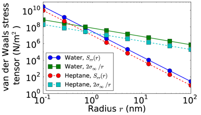
Figure 3: Size dependence of van der Waals surface stress ($\mathcal{S}_{rr}$) and stress due to surface tension ($\sigma_{\infty}$) of a spherical bubble, in water and heptane, respectively. The intersection of the stresses indicates a critical value of radius $r_{cr}$, which is defined to be such that $\mathcal{S}_{rr}=2\sigma_{\infty}/r$. As $r\gg r_{cr}$, surface tension dominates the surface energy of a bubble in the process of homogeneous nucleation. Whereas $r<r_{cr}$, van der Waals stress plays a significant role in surface energy of a micro and nano-sized bubble.

IV Conclusion

Fluctuations of electromagnetic fields lead to radiative energy and momentum transfer between objects. They can be described by the cross-spectral densities of the electromagnetic fields, which are expressed in terms of the dyadic Green’s functions of the vector Helmholtz equation. The radiative energy and momentum transfer between planar objects have been studied during the past decades, while that between other geometries, such as spherical or cylindrical shapes, have not been investigated well. Proximity approximation and/or modified proximity approximation is one commonly used numerical approach to probe the near-field thermal radiation and fluctuation-induced van der Waals pressure between curved surface, but its validity depends strongly on the configurations and sizes of objects.

In this paper, we apply fluctuational electrodynamics directly to evaluate emissivity of thermal radiation and van der Waals contribution to surface energy for various spherical shapes, such as a sphere, a bubble, a spherical shell and a coated sphere, in a homogeneous and isotropic medium. The dyadic Green’s function formalism of thermal radiative transfer and van der Waals stress for different spherical configurations have been developed. We have shown the size dependence and wavelength selectivity of emission spectrum and surface energy of the micro/nanoscale spheres for small radii. The emissivity of sharp peaks can be observed at wavelengths corresponding to the characteristics of the material’s refractive index, and improved as the size of object decreases. van der Waals contribution dominates the surface energy when size of object is reduced to a nanoscopic length scale. The study of fluctuation-induced radiative energy and momentum transfer for spherical shapes has great applications in the nanoscale engineering, e.g., nanoparticles/beads and coated spherical shells, and it deserves further investigation in future.

References

- Planck (2011) M. Planck, The theory of heat radiation (Dover Publications, 2011).
- Zheng (2014) Y. Zheng, Near-field Radiative Momentum, Energy and Entropy Transfer in Fluctuational Electrodynamics, Ph.D. thesis, Columbia University (2014).
- Basu et al. (2009) S. Basu, Z. Zhang, and C. Fu, International Journal of Energy Research 33, 1203 (2009).
- Zheng and Narayanaswamy (2014a) Y. Zheng and A. Narayanaswamy, Physical Review A 89, 022512 (2014a).
- Francoeur et al. (2011) M. Francoeur, S. Basu, and S. J. Petersen, Optics express 19, 18774 (2011).
- Narayanaswamy and Zheng (2013a) A. Narayanaswamy and Y. Zheng, Physical Review B 88, 075412 (2013a).
- Pérez-Madrid et al. (2008) A. Pérez-Madrid, J. M. Rubí, and L. C. Lapas, Physical Review B 77, 155417 (2008).
- Huth et al. (2010) O. Huth, F. Rüting, S.-A. Biehs, and M. Holthaus, The European Physical Journal Applied Physics 50, 10603 (2010).
- Von Werne and Patten (1999) T. Von Werne and T. E. Patten, Journal of the American Chemical Society 121, 7409 (1999).
- Biehs and Greffet (2010) S.-A. Biehs and J.-J. Greffet, Physical Review B 81, 245414 (2010).
- Rephaeli and Fan (2009) E. Rephaeli and S. Fan, Optics express 17, 15145 (2009).
- Avitzour et al. (2009) Y. Avitzour, Y. Urzhumov, and G. Shvets, Phys. Rev. B 79, 045131 (2009).
- Sergeant et al. (2010) N. Sergeant, M. Agrawal, and P. Peumans, Optics Express 18, 5525 (2010).
- Cao et al. (2010) L. Cao, P. Fan, A. P. Vasudev, J. S. White, Z. Yu, W. Cai, J. A. Schuller, S. Fan, and M. L. Brongersma, Nano letters 10, 439 (2010).
- Narayanaswamy et al. (2014) A. Narayanaswamy, J. Mayo, and C. Canetta, Applied Physics Letters 104, 183107 (2014).
- Belosludov and Nabutovskiy (1975) V. Belosludov and V. Nabutovskiy, Zh. eksp. i teor. fiz 68, 2177 (1975).
- Pitaevskii (2006) L. Pitaevskii, Physical Review A 73, 047801 (2006).
- Narayanaswamy and Zheng (2013b) A. Narayanaswamy and Y. Zheng, Physical Review A 88, 012502 (2013b).
- Parsegian (2006) V. A. Parsegian, Van der Waals forces: a handbook for biologists, chemists, engineers, and physicists (Cambridge University Press, 2006).
- Tai (1994) C.-T. Tai, Dyadic Green functions in electromagnetic theory, Vol. 272 (IEEE press New York, 1994).
- Narayanaswamy and Zheng (2014) A. Narayanaswamy and Y. Zheng, Journal of Quantitative Spectroscopy and Radiative Transfer 132, 12 (2014).
- Yla-Oijala and Taskinen (2003) P. Yla-Oijala and M. Taskinen, Antennas and Propagation, IEEE Transactions on 51, 2106 (2003).
- Ottens et al. (2011) R. Ottens, V. Quetschke, S. Wise, A. Alemi, R. Lundock, G. Mueller, D. H. Reitze, D. B. Tanner, and B. F. Whiting, Physical Review Letters 107, 014301 (2011).
- Francoeur et al. (2009) M. Francoeur, M. Pinar Mengüç, and R. Vaillon, Journal of Quantitative Spectroscopy and Radiative Transfer 110, 2002 (2009).
- Dzyaloshinskii et al. (1961) I. E. Dzyaloshinskii, E. Lifshitz, and L. P. Pitaevskii, Physics-Uspekhi 4, 153 (1961).
- Parsegian and Ninham (1973) V. A. Parsegian and B. W. Ninham, Journal of Theoretical Biology 38, 101 (1973).
- Antezza et al. (2008) M. Antezza, L. P. Pitaevskii, S. Stringari, and V. B. Svetovoy, Physical Review A 77, 022901 (2008).
- Sheikholeslami and Ganji (2014) M. Sheikholeslami and D. D. Ganji, Journal of the Brazilian Society of Mechanical Sciences and Engineering , 1 (2014).
- Edalatpour and Francoeur (2014) S. Edalatpour and M. Francoeur, Journal of Quantitative Spectroscopy and Radiative Transfer 133, 364 (2014).
- Sasihithlu and Narayanaswamy (2011) K. Sasihithlu and A. Narayanaswamy, Physical Review B 83, 161406 (2011).
- Zhu et al. (2013) L. Zhu, C. R. Otey, and S. Fan, Physical Review B 88, 184301 (2013).
- Narayanaswamy et al. (2008) A. Narayanaswamy, S. Shen, and G. Chen, Physical Review B 78, 115303 (2008).
- Incardone et al. (2014) R. Incardone, T. Emig, and M. Krüger, EPL (Europhysics Letters) 106, 41001 (2014).
- Otey and Fan (2011) C. Otey and S. Fan, Phys. Rev. B 84, 245431 (2011).
- Otey et al. (2014) C. R. Otey, L. Zhu, S. Sandhu, and S. Fan, Journal of Quantitative Spectroscopy and Radiative Transfer 132, 3 (2014).
- Rytov (1967) S. Rytov, Theory of Electric Fluctuations and Thermal Radiation (Air Force Cambridge Research Center, Bedford, Mass., 1959), Tech. Rep. (AFCRC-TR-59-162, 1967).
- Zheng and Narayanaswamy (2011) Y. Zheng and A. Narayanaswamy, Physical Review A 83, 042504 (2011).
- Hough and White (1980) D. B. Hough and L. R. White, Advances in Colloid and Interface Science 14, 3 (1980).
- Palik (1998) E. D. Palik, Handbook of optical constants of solids, Vol. 3 (Academic press, 1998).
- Lifshitz (1956) E. Lifshitz, Sov. Phys. JETP 2, 73 (1956).
- Narayanaswamy and Chen (2008) A. Narayanaswamy and G. Chen, Physical Review B 77, 075125 (2008).
- Zheng and Narayanaswamy (2014b) Y. Zheng and A. Narayanaswamy, Journal of Physics: Condensed Matter, submitted (2014b).
- (43) NIST Chemistry WebBook (NIST standard reference data), http://webbook.nist.gov/chemistry/ .