Theory of force-extension curve for modular proteins and DNA hairpins

Abstract

We study a model describing the force-extension curves of modular proteins, nucleic acids, and other biomolecules made out of several single units or modules. At a mesoscopic level of description, the configuration of the system is given by the elongations of each of the units. The system free energy includes a double-well potential for each unit and an elastic nearest neighbor interaction between them. Minimizing the free energy yields the system equilibrium properties whereas its dynamics is given by (overdamped) Langevin equations for the elongations, in which friction and noise amplitude are related by the fluctuation-dissipation theorem. Our results, both for the equilibrium and the dynamical situations, include analytical and numerical descriptions of the system force-extension curves under force or length control, and agree very well with actual experiments in biomolecules. Our conclusions also apply to other physical systems comprising a number of metastable units, such as storage systems or semiconductor superlattices.

I Introduction

Nowadays technological advances allow manipulation of single molecules with sufficient precision to study many mechanical, kinetic and thermodynamic properties thereof. Recent reviews of techniques used and results obtained in single-molecule experiments (SMEs) can be found in Refs. rit06jpcm ; KyL10 ; MyD12 . In these experiments, typically the force applied to pull the biomolecule is recorded as a function of its end-to-end distance, thereby producing a force-extension curve (FEC). This FEC characterizes the molecule elasticity and provides information about its processes of folding and unfolding smi96 ; car99 ; lu99 ; fis00 ; lip01 ; bus03 ; man05 ; cao08 . In the following, the end-to-end distance of the biomolecule is referred to as the total length length . The force–extension curves are different depending on whether the total length or the force are controlled. When the total length of the protein is used as a control parameter (length-control), the unfolding transition is accompanied by a drop in the measured force and a sawtooth pattern is the typical force–extension curve fis00 ; car99 ; lip01 ; bus03 ; lip02 . When the force is the control parameter (force-control), unfolding of several or all single protein domains may occur at a constant value of the force hug10 . Other questions are related to the rate at which the control parameter (length or force) sweeps the force–extension curve: depending on the loading rate, stochastic jumps between folded and unfolded protein states may be observed rit06jpcm ; lip01 ; man05 ; lip02 ; hug10 .

The analysis of the force vs. extension curves provides valuable information about the polyprotein, the DNA or the RNA hairpin. Let us consider atomic force microscope (AFM) experiments in which a modular protein comprising a number of identical folds (modules or units) is pulled at a certain rate (length-control) car99 ; fis00 . The typical value of the force $F_{c}$ at which the unfolding takes place is related to the mechanical stability of the units: a larger value of the force is the signature of higher stability. Nevertheless, it should be stressed that the unraveling of a domain is a stochastic event and occurs for forces within a certain range. A second feature of the sawtooth FEC is the spacing between consecutive force peaks. This spacing is directly related to the difference of length between the folded and unfolded configurations of one unit. This is the reason that the peaks of the FEC of artificially engineered modular proteins are regularly spaced. A typical example is I27₈, composed of eight copies of immunoglubulin domain 27 from human cardiac titin. The spacing between peaks for this protein is $28.4\pm 0.3$nm at an unfolding force of $204\pm 26$pN car99 ; fis00 . This length increment is found by fitting several peaks of the FEC with the worm-like chain (WLC) model of polymer elasticity bus94 ; mar95 . More recently, force-controlled AFM experiments with a I27 single-module protein have been reported ber10 ; ber12 . These experiments provide data free from the module to module variations that even an artificially engineered polyprotein has. Berkovich et al. have interpreted their results using a simple Langevin equation model that includes an effective potential with two minima for a range of the applied force ber10 .

The thermodynamics of pulling experiments is well established under both force and length control. For controlled force, the relevant thermodynamic potential is a Gibbs-like free energy, whereas for controlled length it is a Helmholtz-like free energy KSyB03 ; man05 ; RByK06 . Interestingly, the sawtooth structure of the FEC of biomolecules is already present at equilibrium, as shown very recently in a simple model with a Landau-like free energy pra13 . However, the control parameter in real experiments with biomolecules (force or length) changes usually with time at a finite rate rit06jpcm ; MyD12 ; fis00 ; lip01 ; lip02 ; man05 ; hug10 ; HBFSByR10 . Knowledge of these dynamical situations is not as complete as in the equilibrium case. Under force control, we can write a Langevin equation (or the associated Fokker-Planck equation) in which noise amplitude and effective friction are linked by a fluctuation-dissipation relation, as done in Refs. ber10 ; RRyV05 . On the other hand, under length control, the situation is more complex: the force is no longer a given function of time but an unknown that must be calculated by imposing the length constraint. This has lead to the proposal of simple dynamical algorithms such as the quasi-equilibrium algorithm of Ref. man05 . While being successful in reproducing experimentally observed behavior, these algorithms do not correspond to the integration of well-defined evolution equations.

In some cycling experiments, the biomolecule is switched between the folded and unfolded configurations, at a certain switching rate rit06jpcm ; lip01 ; lip02 ; man05 ; hug10 ; HBFSByR10 . After Liphardt et al., we call such a process a stretching/relaxing or an unfolding/refolding cycle lip01 ; lip02 . The unfolding typically occurs at a force $F_{u}$ that is larger than the refolding force $F_{r}$. Therefore, some hysteresis is present and, moreover, the unfolding (refolding) force typically increase (decrease) with the pulling rate. A reversible curve in which $F_{u}=F_{r}=F_{c}$ is only observed for a small enough rate. Some authors have claimed that this is a signature of irreversible non-equilibrium behavior and thus used these experiments to test non-equilibrium fluctuation theorems lip02 ; PKTyS03 ; CRJSTyB05 ; HyS10 . On the other hand, for a simple model for which only the force-controlled situation could be analyzed pra12 , it has been found that the observed behavior in biomolecules can be understood as the system sweeping a certain part of the metastable equilibrium region of the FEC that surrounds $F_{c}$. In this way, the system is exploring metastable minima of the system free energy landscape. One of the main goals of this work is to determine if this physical picture also holds for length-controlled experiments.

In this paper, we add two important ingredients of real biomolecule pulling experiments to a simple model with independent domains and Landau-like free energy whose equilibrium analysis is given in Ref. pra13 . We add: (i) dynamical effects and (ii) interacting units. Dynamical effects are introduced by means of Langevin or Fokker-Planck equations, both under force and, most interestingly, length control. Therefrom, we can carry out a systematic investigation of the dynamical FEC, when the control parameter (force or length) is varied at a finite rate. The simplest way to introduce interaction between modules is via a harmonic potential trying to drive them to global equilibrium. In this way, the creation of bubbles, that is, regions of unfolded modules inside regions of folded ones, has a free energy cost. This is expected to be most relevant for systems in which the unfolding/refolding of units is mainly sequential, as in the unzipping of DNA hairpins rit06jpcm . Interestingly, the complex and force-sensitive behavior of polyproteins observed in force-clamp experiments has been recently explained by sequential unfolding BCyP14 .

The main ingredients of our model are bistability of protein modules and, in the length-controlled case, a global constraint that introduces a long-range interaction among modules. These features are quite general in physics, as they appear in many different fields. For instance, many particle storage systems such as the storage of lithium in multi-particle electrodes of rechargeable lithium-ion batteries dre10 ; dre11 , air storage in interconnected systems of rubber balloons dre11cmt , or voltage biased weakly coupled semiconductor superlattices GHMyP91 ; RTGyP02 ; BGr05 ; BT10 ; BHGyT12 . Throughout the paper, the analogies and differences that arise in these different physical situations will be discussed.

The rest of the paper is as follows. The model we use is described in Section II, in which we write down both the Langevin and the Fokker-Planck equations in Secs. II.1 and II.2, respectively. In Section III, we investigate an ideal modular protein comprising many identical, non-interacting, units. In Sec. III.1, we show that the equilibrium FEC corresponding to our Landau-like double-well free energy has multiple branches. Statistical mechanics considerations determine the stability of the equilibrium branches for: (a) force-control in Sec. III.2, and (b) length-control in Sec. III.3. We also consider dynamical situations when the control parameter (either force or length) varies at a finite rate. Section IV deals with a real chain, in which the nearest neighbor modules interact via an extra harmonic term. First, we study the equilibrium situation in Sec. IV.1, in which we show that the size of the branches is reduced, as compared to the ideal case. Sections IV.2, IV.3, and IV.4 analyze the changes that the dynamics brings to the equilibrium picture by considering deterministic dynamics, quenched disorder and finite temperature dynamics (thermal noise), respectively. Final remarks are made in Section V. Appendix A explains unfolding and refolding under length control using a more realistic potential, whereas Appendices B and C deal with some technical aspects not covered in the main text.

II Model

To be specific, let us consider AFM unfolding of modular proteins: They are stretched between the tip of the microscope cantilever and a flat, gold-covered substance (platform), whose position is externally controlled. The forces acting on the molecule bend the cantilever which, in turn, determines the applied force with pN precision. See Fig. 1 of Refs. MyD12, or  fis00, for an idealized situation. In force-controlled experiments with a single module protein, the free energy of an extending protein comprises at least two distinct components, an entropic term that accounts for chain elasticity and an enthalpic component that includes the short-range interactions arising between the neighboring amino acids as the protein contracts ber10 ; ber12 . In a certain force range, these two components cause the single-module free energy to have two minima, corresponding to the folded and unfolded states of the domain ber10 .

Let us consider a system comprising $N$ modules. The $j$-th module extends from $x_{j}$ to $x_{j+1}$, so that its extension is $\eta_{j}=x_{j+1}-x_{j}$, $j=1,\ldots,N$. The configuration $\bm{\eta}=\{\eta_{j}\}$ defines the polyprotein state at a mesoscopic level of description. When isolated, the free energy of the $j$-th unit is $a(\eta_{j};Y,\delta_{j})$, a double-well potential whose minima correspond to the folded and unfolded states discussed above. $Y$ is the set of relevant intensive parameters, like the temperature $T$ and the pressure $p$ of the fluid (thermal bath) surrounding our system. The parameter $\delta_{j}$ accounts for the slight differences from unit to unit: $\delta_{j}=0$, $\forall j$, if all units are identical and thus no quenched disorder is present in the system.

As part of the tertiary structure of the polyprotein, modules are weakly interconnected by linkers in a structure-dependent way HyD12 . It seems reasonable that this weak interaction acts on the unfolding/refolding time scale and tries to bring the extensions of the modules to a common value, corresponding to global mechanical equilibrium. For the sake of simplicity, we model the linkers as harmonic springs. Thus the system free energy $\mathit{A}$ for a given configuration of module extensions $\bm{\eta}$ is

$$\mathit{A}(\bm{\eta};Y)=\sum_{j=1}^{N}a(\eta_{j};Y,\delta_{j})+\sum_{j=2}^{N}\frac{k_{j}(Y)}{2}(\eta_{j}-\eta_{j-1})^{2}.$$ (1)

If all the linkers are identical, $k_{j}=k$ for all $j=2,\ldots,N$, and the elastic constants may depend on the intensive parameters. The length $\mathit{L}$ of a polyprotein in a configuration $\bm{\eta}$ is

$$\mathit{L}(\bm{\eta})=\sum_{j=1}^{N}\eta_{j}.$$ (2)

The experiments are carried out at either force-controlled or length-controlled conditions. Firstly, we analyze case (i), in which a certain external force $F=F(t)$ is applied to the ends of the protein or DNA hairpin. For a detailed discussion of how this is achieved in real experiments, see for example Refs. hug10 (ch. 6) and FLMHHyR11 for the optical tweezers case, and OHCyF01 ; FyL04 for the AFM case. In our simplified theoretical approach, we only have to add a term

$$\Delta U_{\text{fc}}(\bm{\eta};F)=-FL(\bm{\eta})=Fx_{1}-Fx_{N+1}$$ (3)

to the free energy $\mathit{A}(\bm{\eta})$. In this way, we obtain a Gibbs free energy $\mathit{G}(\bm{\eta};Y,F)=\mathit{A}(\bm{\eta},Y)+\Delta U_{\text{fc}}=\mathit{A}(\bm{\eta},Y)-F\mathit{L}(\bm{\eta})$,

$$\mathit{G}(\bm{\eta};Y,F)=\sum_{j=1}^{N}g(\eta_{j};Y,F,\delta_{j})+\sum_{j=2}^{N}\frac{k_{j}(Y)}{2}(\eta_{j}-\eta_{j-1})^{2},$$ (4a)

$$g(\eta_{j};Y,F,\delta_{j})=a(\eta_{j};Y,\delta_{j})-F\eta_{j}.$$ (4b)

Note that we are not taking into account the limited bandwidth of the feedback device that controls force in real experiments; we are assuming that the desired force program $F(t)$ is perfectly implemented. Secondly, we investigate the length-controlled situation, case (ii). For a schematic representation of the experimental situation, see for instance Fig. 1 of Ref. MyD12, : The length $L(t)$ between the base of the cantilever and the platform is the externally controlled quantity. On the other hand, the cantilever tip deflects a certain distance $\Delta x$ from its base, such that $\Delta x+\mathit{L}(\eta)=L(t)$. If the stiffness (spring constant) of the cantilever is $\chi_{\text{lc}}$, we have an extra harmonic term in the potential $U_{\text{lc}}=\chi_{\text{lc}}(\Delta x)^{2}/2$, that is,

$$\Delta U_{lc}(\bm{\eta};L)=\frac{\chi_{\text{lc}}}{2}\left[L(\bm{\eta})-L(t)\right]^{2},$$ (5)

Therefore, an extra force $\Delta F_{lc}=-\chi_{\text{lc}}[L(\bm{\eta})-L(t)]$ acts over each unit, trying to keep the polyprotein length equal to $L(t)$: The larger $\chi_{\text{lc}}$, the better the length-control is, as expected on intuitive grounds and explicitly shown in PKTyS03 . In this paper, with the exception of Appendix A, we assume perfect length control, that is, we consider the limit $\chi_{\text{lc}}\to\infty$ that implies $L(\bm{\eta})-L(t)\to 0$ over the time evolution of the units and a finite value of the corresponding extra force $\Delta F_{lc}$. In other words, $\Delta F_{lc}$ tends to a limiting value $F$ that depends on the prescribed length $L(t)$. This unknown value is the force required to attain the total length $L(t)$, and it has to be calculated by imposing the constraint $\sum_{i}x_{i}=L$. The effect of this limit on the relevant thermodynamic potential for the length-controlled case $A+\Delta U_{lc}$ shall be discussed in the section on Fokker-Planck description of the dynamics.

Finally, we would like to stress that the present model has some similarities with the more complicated one proposed by Hummer and Szabo for the unfolding of polyproteins several years ago, see Appendix C of Ref. HyS03 . In addition to the module extensions $\eta_{j}$, these authors consider the module centers of mass $r_{j}$ as independent unknowns. These variables interact through a quadratic potential that yields a linear restoring force whenever $r_{j+1}-r_{j}$ departs from $\frac{\eta_{j+1}+\eta_{j}}{2}$. The site potential for the module extensions is the sum of a WLC potential and a harmonic potential HyS03 , instead of the double-well potential we consider in the main text or the asymmetric potential we consider in Appendix A. Moreover, Hummer and Szabo introduce a WLC linker that connects the polyprotein with the length-controlling device, which is absent in our model.

II.1 Langevin dynamics

The extensions $\eta_{j}$ obey coupled Langevin equations with the appropriate thermodynamic potential. The friction coefficient and the amplitude of the white noise are related by a fluctuation-dissipation theorem. The source for both the friction and the stochastic force is the fluid the modules are immersed in, which is assumed to remain in equilibrium at temperature $T$. We assume that the modules’ inertia can be neglected and thus their evolution equations are overdamped,

$$\gamma_{j}\dot{\eta}_{j} = F-\frac{\partial}{\partial\eta_{j}}\mathit{A}(\bm{\eta};Y)+\sqrt{2T\gamma_{j}}\,\xi_{j}(t),$$ (6a)

$$\langle\xi_{j}(t)\rangle\!=\!0,\,\langle\xi_{j}(t)\xi_{l}(t^{\prime})\rangle\!=\!\delta_{jl}\,\delta(t-t^{\prime}),\,j\!=\!1,\ldots,N.$$ (6b)

Here $\gamma_{j}$ is the friction coefficient for the $j$-th module, and we measure the temperature in units of energy ($k_{B}=1$). In general, the friction coefficients $\gamma_{j}$ may depend on the system configuration $\bm{\eta}$, if hydrodynamic interactions play a significant role in the considered unfolding scenario. For the sake of simplicity, we do not consider this possibility in the present paper. In this respect, it is interesting to remark that, in the more complicated model of Ref. HyS03 , module centers of mass and extensions satisfy Langevin equations with different extension-dependent diffusion coefficients.

Our presentation of the model above implies that the Langevin equations (6) are valid both in force-controlled and length-controlled experiments, but (i) in force-controlled experiments, $F=F(t)$ is the known force program, whereas (ii) in length-controlled ones we have $\mathit{L}(\bm{\eta})=L(t)$. We differ the discussion on the experimental situation with an “imperfect” length control (because of the finite value of the stiffness $\chi_{\text{lc}}$ of the device controlling the length) to the next section on the equivalent Fokker-Planck description of the dynamics. For perfect length control, $F(t)$ is determined by imposing the constraint $L(\bm{\eta})=L$, which yields

$$F=\frac{\gamma}{N}\!\left(\frac{dL}{dt}+\sum_{j=1}^{N}\frac{1}{\gamma_{j}}\frac{\partial\mathit{A}(\bm{\eta};Y)}{\partial\eta_{j}}-\sum_{j=1}^{N}\sqrt{\frac{2T}{\gamma_{j}}}\xi_{j}\right)\!\!.$$ (7a)

$$\gamma^{-1}=\frac{1}{N}\sum_{j=1}^{N}\gamma_{j}^{-1}.$$ (7b)

The parameter $\gamma$ is an average friction coefficient. In the case of identical units, $\gamma_{j}=\gamma$, $\forall j$. We split $F$ in two terms, a “macroscopic term” $F_{FP}$ and a “fluctuating term” $\Delta F$, as follows:

$$F=F_{\text{FP}}+\Delta F,$$ (8a)

$$F_{\text{FP}} = \frac{\gamma}{N}\left[\frac{dL}{dt}+\sum_{j=1}^{N}\frac{1}{\gamma_{j}}\frac{\partial\mathit{A}(\bm{\eta};Y)}{\partial\eta_{j}}\right],$$ (8b)

$$\Delta F = -\frac{\gamma}{N}\sum_{j=1}^{N}\sqrt{\frac{2T}{\gamma_{j}}}\xi_{j}.$$ (8c)

We prove in Sec. II.2 that $F_{FP}$ is the force appearing in the flux term of the Fokker-Plack equation. Note that for any $N$, $\langle\Delta F\rangle=0$ and then $\langle F\rangle=\langle F_{\text{FP}}\rangle$. Furthermore, $\Delta F$ is a sum of Gaussian variables, and thus its statistical properties are completely given by its first two moments. It can be easily shown that $\langle\Delta F(t)\Delta F(t^{\prime})\rangle=N^{-1}\gamma\,\delta(t-t^{\prime})$, its variance tends to zero as $N^{-1}$, which is the typical behavior of fluctuating quantities in statistical mechanics. Even so, it should be noted that in biomolecules $N$ is not necessarily very large and certainly not of the order of Avogadro’s number, and thus fluctuations play a major role. In force–extension experiments, the length is usually uniformly increased/decreased with time $t$, $dL/dt=\mu$ with a constant $\mu$.

It is convenient to render our equations dimensionless. We set the length unit $[\eta]$ equal to the difference between the extensions of the two free energy minima of a single unit for a certain applied force. It is natural to adopt the critical force, at which the two minima are equally deep, as the unit of force, $[F]=F_{c}$. The parameters $[\eta]$ and $[F]$ depend on the specific choice of the double-well potential $a(\eta;Y,0)$. The free energy unit is then $[F]\,[\eta]$. We select the time scale as $[t]=\gamma[\eta]/[F]$, where $\gamma$ is the typical friction coefficient experienced by the units. The typical value of $\gamma$ can be obtained from the value of the diffusion coefficient $D=T/\gamma$ of a single module protein being stretched ber12 . In principle, we introduce a new notation for the dimensionless variables, $F^{*}=F/[F]$, etc. but, in order not to clutter our formulas, we drop the asterisks in the remainder of the paper.

II.2 Fokker-Planck equation and equilibrium distributions

In force controlled experiments, $F(t)$ is a given function of time, and the set of Langevin equations (6a) is equivalent to the following Fokker-Planck equation for the probability density $\mathcal{P}(\bm{\eta},t)$ of finding the system with extension values $\bm{\eta}=\{\eta_{1},\ldots,\eta_{N}\}$ at time $t$,

$$\frac{\partial}{\partial t}\mathcal{P}=\sum_{j=1}^{N}\frac{1}{\gamma_{j}}\frac{\partial}{\partial\eta_{j}}\left[\frac{\partial\mathit{G}}{\partial\eta_{j}}\mathcal{P}\right]+T\sum_{j=1}^{N}\frac{1}{\gamma_{j}}\frac{\partial^{2}\mathcal{P}}{\partial\eta_{j}^{2}}.$$ (9)

where $\mathit{G}=\mathit{A}-F\mathit{L}$, as given by Eq. (4a). If the force $F$ is kept constant, Eq. (9) has a stationary solution, which is the statistical mechanics prescription,

$$\mathcal{P}^{\text{eq}}(\bm{\eta})\propto e^{-\mathit{G}(\bm{\eta};Y,F)/T}.$$ (10)

Therefore, the equilibrium values of the module extensions $\bm{\eta}^{\text{eq}}$ are the functions of $F$ that maximize $\mathcal{P}$ or, equivalently, minimize $\mathit{G}$, that is, they verify

$$\left.\left(\frac{\partial\mathit{G}}{\partial\eta_{j}}\right)_{\!\!Y,F}\right|_{\text{eq}}=0\,\,\Rightarrow\,\,\eta_{j}=\eta_{j}^{\text{eq}}(Y,F),\quad j=1,\ldots,N.$$ (11)

If there is only one minimum, this is the equilibrium configuration. If there is more than one, the absolute minimum is the thermodynamically stable configuration, while the other minima correspond to metastable states in the thermodynamic sense. For each equilibrium configuration, either stable or metastable, the equilibrium value of the free energy $\mathit{G}$ is

$$\mathit{G}^{\text{eq}}(Y,F)=\mathit{G}(\bm{\eta}^{\text{eq}}(Y,F);Y,F).\$$ (12)

Taking into account Eq. (11), we have

$$\left(\frac{\partial\mathit{G}^{\text{eq}}}{\partial F}\right)_{\!\!Y}\!\!\!=\!\!\ \left.\left(\frac{\partial\mathit{G}}{\partial F}\right)_{\bm{\eta},Y}\right|_{\text{eq}}\!\!\!\!=\!-\sum_{j=1}^{N}\eta_{j}^{\text{eq}}(Y,F)=\!-\mathit{L}^{\text{eq}}(Y,F),$$ (13)

which gives the equilibrium FEC under force control.

Let us consider now the length control situation. In the experiments, the device controlling the length of the system does not have an infinite stiffness and thus the length-control is not perfect, as discussed above (see also PKTyS03 and Appendix A). Had we taken into account this finite value of the stiffness $\chi_{\text{lc}}$, the Fokker-Planck equation would have been obtained by substituting the Gibbs free energy $G\equiv A+\Delta U_{\text{fc}}$ in Eq. (9) by the corresponding thermodynamic potential $A+\Delta U_{\text{lc}}$. Thus, the stationary solution of this Fokker-Planck equation would be the equilibrium distribution $\mathcal{P}^{\text{eq}}(\bm{\eta};Y,L)\propto\exp[-(\mathit{A}(\bm{\eta};Y)+\Delta U_{lc}(\bm{\eta};L))/T]$. Of course, in the limit as $\chi_{\text{lc}}\to\infty$, the variance of the Gaussian factor $\exp[-\Delta U_{lc}(\bm{\eta};L)/T]$ vanishes and this factor tends to a delta function $\delta(L(\bm{\eta})-L)$ giving perfect length control.

In the case of perfect length control, the correct Fokker-Planck equation can be obtained by taking the limit as $\chi_{\text{lc}}\to\infty$, but here we follow an alternative route. We calculate the first two moments of the extensions $\bm{\eta}$, taking into account that not all the extensions $\eta_{j}$ are independent and that the force $F$ is given by eq. (7a),

$$\frac{\partial}{\partial t}\mathcal{P} = \sum_{j=1}^{N}\frac{1}{\gamma_{j}}\frac{\partial}{\partial\eta_{j}}\left[\left(\frac{\partial\mathit{A}}{\partial\eta_{j}}-F_{\text{FP}}\right)\mathcal{P}\right]$$ (14)

$$+T\sum_{j=1}^{N}\frac{1}{\gamma_{j}}\sum_{k=1}^{N}\left(\delta_{jk}-\frac{\gamma}{N\gamma_{k}}\right)\frac{\partial^{2}}{\partial\eta_{j}\partial\eta_{k}}\mathcal{P}.$$

Here $F_{\text{FP}}$ is given by Eq. (8b). If the length is kept constant, $dL/dt=0$, Eq. (14) has a stationary solution,

$$\mathcal{P}^{\text{eq}}(\bm{\eta};Y,L)\propto\delta(L(\bm{\eta})-L)\;e^{-\mathit{A}(\bm{\eta};Y)/T},$$ (15)

as can be easily verified by inserting (15) into (14). This means that $\mathit{A}$ is the relevant potential for the statistical mechanics description at equilibrium, as was expected. Eq. (15) is consistent with the limit as $\chi_{\text{lc}}\to\infty$ of the equilibrium distribution for realistic length control, as already discussed above.

To obtain the equilibrium values for the extensions, we look for the minima of $\mathit{A}$ with the constraint given by the delta function in (15), $\mathit{L}(\bm{\eta})=L$. We have to introduce a Lagrange multiplier $F$ and look for the minima of $\mathit{A}-F\mathit{L}$, that is, the same minimization as in the force-controlled case. However, the Lagrange multiplier is an unknown that must be calculated at the end of the process by imposing the constraint, $F=F(L)$. This Lagrange multiplier is, from a physical point of view, the force that must be applied to the system in order to have the desired length. The equilibrium extensions $\eta_{j}^{\text{eq}}(L)$ are thus given by the solutions of

$$\left.\left(\frac{\partial\mathit{A}}{\partial\eta_{j}}\right)_{Y}\!\right|_{\text{eq}}\!\!=F,\,\,j=1,\ldots,N;\,\,\sum_{j=1}^{N}\eta_{j}^{\text{eq}}(Y,F)=L.$$ (16)

The last equation gives the FEC, $L=L(Y,F)$ or $F=F(Y,L)$, from which we obtain $\eta^{\text{eq}}=\eta^{\text{eq}}(Y,L)$. The thermodynamic potential $\mathit{A}^{\text{eq}}$ is the Legendre transform of $\mathit{G}^{\text{eq}}$ with respect to $F$. In fact, the equilibrium value of $\mathit{A}$, $\mathit{A}^{\text{eq}}(Y,L)=\mathit{A}(\bm{\eta}^{\text{eq}}(Y,L);Y)$, verifies that

$$\left(\frac{\partial\mathit{A}^{\text{eq}}(Y,L)}{\partial L}\right)_{Y}=F.$$ (17)

The proper variables for $\mathit{A}^{\text{eq}}$ are the set of intensive parameters $Y$ (temperature $T$, pressure $p$, $\ldots$ of the fluid in which the polyprotein is immersed) and the extensive length $L$ footnote1 , while the proper variables for $\mathit{G}^{\text{eq}}$ are all intensive, $Y$ and $F$. In this sense, $\mathit{A}^{\text{eq}}$ plays the role of Helmhotz free energy, while $\mathit{G}^{\text{eq}}$ is the analogous of Gibbs free energy. It should be stressed that (i) however, different notations are found in the literature for these two thermodynamic potentials; (ii) as in the case of magnetic systems tho88 , there is a difference of sign with respect to the usual free energy terms with the pressure $p$ and the volume $V$.

The fluctuation theorems for Markov processes described by the Langevin (or the equivalent Fokker-Planck) equations have been thoroughly analyzed in Ref. CCyJ06 . The results therein are directly applicable to the Fokker-Planck equations derived here for the force-controlled and the realistic (finite $\chi_{\text{lc}}$) length-controlled cases. When the controlled parameter (either force or length) is kept constant (time-independent), detailed balance applies and the corresponding stationary distributions are equilibrium (canonical) ones (in the terminology of section 2 in Ref. CCyJ06 ). In the limit as $\chi_{\text{lc}}\to\infty$, we expect this result to be still valid on physical grounds, but further mathematical work would be necessary to establish it rigorously: Some of the matrices defined in CCyJ06 become singular and thus have no inverse. This is a point that certainly deserves further investigation, but it is out of the scope of the present paper.

III The ideal chain

In this Section, we analyze the case of an ideal chain, in which the identical units do not interact either among themselves or with the cantilever/platform, $k_{j}=0$ and $\delta_{j}=0$ for all $j$ pra13 . We analyze the equilibrium situation and thus solve the minimization problems for the force-controlled and length-controlled cases of the previous section. We also investigate the dynamical situation arising in processes in which the force or length varies in time at a finite rate, and compare these dynamical FECs to the equilibrium ones.

III.1 Double-well potential. Equilibrium branches.

In order to keep the notation simple, we omit the dependence on the intensive parameters $Y$ of the free energy parameters. As a minimal model, we consider the polynomial form, à la Landau, for the free energy pra13

$$\mathit{A}(\bm{\eta})=\sum_{j=1}^{N}a(\eta_{j}),\quad a(\eta)=F_{c}\eta-\alpha\eta^{2}+\beta\eta^{4}.$$ (18)

The parameters $F_{c}$, $\alpha$ and $\beta$ are all positive functions of the intensive parameters $Y$. Specifically, $F_{c}$ plays the role of the critical force, above (below) which the unfolded (folded) configuration is the most stable one, as shown in what follows. The possible equilibrium extensions $\eta^{\text{eq}}$ are the minima of $a(\eta)-F\eta$,

$$a^{\prime}(\eta^{(i)})=F$$ (19)

or, equivalently,

$$-2\alpha\eta^{(i)}+4\beta\left(\eta^{(i)}\right)^{3}=\varphi,\quad\varphi\equiv F-F_{c}.$$ (20)

We have introduced the notation $\eta^{(i)}$ because Eq. (20) has three solutions in the metastability region, given by $|\varphi|=|F-F_{c}|<\varphi_{0}=(2\alpha/3)^{3/2}\beta^{-1/2}$. We set the indexes by choosing $\eta^{(1)}<\eta^{(2)}<\eta^{(3)}$. They depend on the force $F$ through $\varphi$ (and on the intensive variables $Y$ through $\{\alpha,\beta,F_{c}\}$). The extensions $\eta^{(1)}(\varphi)$ and $\eta^{(3)}(\varphi)$ are locally stable because they correspond to minima of $a_{j}-F\eta_{j}$, while $\eta^{(2)}(\varphi)$ corresponds to a maximum and is therefore unstable. The curvatures at the folded and unfolded states are $\chi^{(i)}(\varphi)=a^{\prime\prime}(\eta^{(i)}(\varphi))=12\beta[\eta^{(i)}(\varphi)]^{2}-2\alpha$, $i=1,3$. Both curvatures (i) are positive in the metastability region and (ii) vanish at their limits of stability, $\chi^{(1)}$ ($\chi^{(3)}$) at $\varphi=\varphi_{0}$ ($\varphi=-\varphi_{0}$).

The situation is similar to that analyzed by Landau landau for a second order phase transition under an external field, with $\eta$ and $\varphi=F-F_{c}$ playing the role of the order parameter and the external field, respectively. At the critical force $\varphi=0$, the stable equilibrium values of the extensions are

$$\eta^{(3)}_{c}=-\eta^{(1)}_{c}=\left(\frac{\alpha}{2\beta}\right)^{1/2}.$$ (21)

They are equiprobable, since $g(\eta)=a-F\eta$ is an even function of $\eta$ for $F=F_{c}$, and $g^{(1)}=a^{(1)}-F_{c}\eta^{(1)}=g^{(3)}=a^{(3)}-F_{c}\eta^{(3)}$, where we have introduced the notation $a^{(1)}\equiv a(\eta^{(1)})$, $a^{(3)}\equiv a(\eta^{(3)})$, $g^{(1)}\equiv g(\eta^{(1)})$, and $g^{(3)}\equiv g(\eta^{(3)})$. For $F\neq F_{c}$, the “field” $\varphi$ favors the state with $\text{sgn}(\varphi)=\text{sgn}(\eta)$. In fact, at the limit of stability we have that $g^{(1)}=-13\alpha^{2}(6\beta)^{-1}$ for $\varphi=-\varphi_{0}$ (or $g^{(3)}=-13\alpha^{2}(6\beta)^{-1}$ for $\varphi=\varphi_{0}$). Therefore, in the metastability region $|\varphi|<\varphi_{0}$, we have the following picture: For $F<F_{c}$, the thermodynamically stable state is the folded one $\eta^{(1)}<0$ and the unfolded one $\eta^{(3)}>0$ is metastable. For $F>F_{c}$, the situation is simply reversed. On the other hand, the folded $\eta^{(1)}$ (unfolded $\eta^{(3)}$) state also exists for forces below (above) the metastability region $\varphi<-\varphi_{0}$ ($\varphi>\varphi_{0}$). In their respective regions of existence, both locally stable extensions $\eta^{(1)}$ and $\eta^{(3)}$ are increasing functions of $\varphi$ (or $F$), since Eq. (19) implies that $\chi^{(k)}(\varphi)d\eta^{(k)}/d\varphi=1$. At zero force, one module can be folded or unfolded if $\varphi_{0}>F_{c}$, while we have only the folded state if $\varphi_{0}<F_{c}$.

Either module can be either folded or unfolded in the metastability region, and thus a FEC with $N+1$ branches shows up, as seen in Fig. 1. The $J$-th branch of the $F-L$ curve corresponds to $J$ unfolded modules and $N-J$ folded ones, $J=0,\ldots,N$. Since there is no coupling among the units, the equilibrium value of $\mathit{A}$ over the $J$-th branch is

$$\mathit{A}_{J}^{\text{eq}}=(N-J)a^{(1)}+Ja^{(3)}.$$ (22a)

The corresponding length is

$$\mathit{L}_{J}=(N-J)\eta^{(1)}+J\eta^{(3)}\!.$$ (22b)

Both $\mathit{A}_{J}^{\text{eq}}$ and $\mathit{L}_{J}$ are functions of $F$ and the intensive parameters $Y$ through the equilibrium extensions. Eq. (22b) is the FEC, both for the force and length controlled cases. In Fig. 1, we have normalized the lengths with

$$\Delta\mathit{L}_{c}=\mathit{L}_{N}(F_{c})-\mathit{L}_{0}(F_{c})=N\left(\eta^{(3)}_{c}-\eta^{(1)}_{c}\right),$$ (23)

which is the difference of lengths between the completely unfolded branch ($J=N$) and the completely folded one ($J=0$) at the critical force. It is interesting to note that similar multistable equilibrium curves appear in quite different physical systems: from storage systems dre10 ; dre11 ; dre11cmt to semiconductor superlattices GHMyP91 ; RTGyP02 ; BGr05 ; BT10 ; BHGyT12 . For instance, see Fig. 3 of Ref. dre10 and Fig. 6 of Ref. dre11 for the chemical potential vs. charge curve in storage systems, and Fig. 8.13 of Ref. BT10 for the current-voltage curve of a superlattice.

As discussed in the previous section, we have chosen $[F]=F_{c}=1$ and $[\eta]=\eta^{(3)}_{c}-\eta^{(1)}_{c}=1$ as units of force and length. Using Eq. (21), $\beta=2\alpha$ and $\eta^{(3)}_{c}=-\eta^{(1)}_{c}=1/2$. Moreover, the folded state $\eta^{(1)}$ is the most stable one at zero force. This means that the unstable state $\eta^{(2)}$ is closer to the metastable state $\eta^{(3)}$ for the simple Landau potential we are using note . For the sake of concreteness, we take $\eta^{(2)}-\eta^{(1)}=0.9(\eta^{(3)}-\eta^{(1)})$ at zero force, which leads to $\alpha=273^{3/2}/1672\approx 2.697787$ and $\varphi_{0}=91^{3/2}/836=1.038378$. It should be stressed that all the normalized plots in this section are independent of this particular choice of parameters. A more conventional definition of protein length could be to select at zero force (a) zero extension for the folded modules (b) the difference between the unfolded and folded configurations as the length unit. This ‘physical’ definition would give a nondimensional extension

$$u=\frac{\eta-\eta^{(1)}(F=0)}{\eta^{(3)}(F=0)-\eta^{(1)}(F=0)},$$ (24a)

and a polyprotein length

$$L_{u}=\frac{-N\eta^{(1)}(F=0)+\sum_{j=1}^{N}\eta_{j}}{\eta^{(3)}(F=0)-\eta^{(1)}(F=0)}\!\!=\frac{19N}{30}+\frac{\sqrt{273}}{15}L,$$ (24b)

respectively. At zero force, the module extensions are $u^{(1)}=0$, $u^{(2)}=0.9$ and $u^{(3)}=1$. The length $L_{u}$ is typically positive for $F>0$, that is, for $\varphi>-F_{c}$.

We expect that the simple Landau-like free energy given by Eq. (18) should be relevant to investigate qualitatively the FECs for forces/lengths close to the metastability region. In particular, this minimal choice does not account for the existence of a maximum length of the polymer, its so-called contour length length , a fact that becomes significant for high forces. In order to study the whole range of forces and/or try to describe quantitatively the experiments, we should use a more realistic potential, such as that proposed by Berkovich et al. ber10 or modifications thereof. We did this in Ref. BCyP14 to understand the stepwise unfolding observed in force-clamp experiments. The simpler potential used in this paper suffices for: (i) showing that the key aspects of the experimental behavior observed in the unfolding/refolding region can be understood within a minimal model, and (ii) establishing connections with other physical systems such as storage devices dre10 ; dre11 ; dre11cmt or semiconductor superlattices GHMyP91 ; RTGyP02 ; BGr05 ; BT10 ; BHGyT12 that have similar behavior in the metastability region. We briefly investigate an asymmetric potential in Appendix A to understand why the experimentally observed FEC corresponding to unfolding under length-control is reproduced by the Landau-like potential whereas the FEC corresponding to refolding is not, see Sec. III.3 for details.

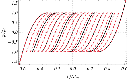
Figure 1: Normalized FECs for $N=8$ (solid black) and $N=20$ (dashed red). Zero length corresponds to having half of the units unfolded at $F=F_{c}$. There are $N+1$ branches in the metastability region $|\varphi/\varphi_{0}|<1$, with the number of unfolded units $J$ increasing from left to right. The first ($J=0$) and last ($J=N$) branches are independent of $N$. Note that the branches become denser as $N$ increases, and also the up-down and left-right symmetry thereof. These symmetries stem from the simple form of the Landau-like free energy (18), and thus they are not present if a more realistic potential is considered, see Appendix A.

III.2 Force control

In force-controlled experiments, the Gibbs free energy is the relevant thermodynamic potential because it appears in the equilibrium distribution (10). As discussed in Sec. II.2, the stable state corresponds to the absolute minimum of $\mathit{G}$. All the units in our ideal chain are independent under force control. Therefore, by increasing quasi-statically the force, the equilibrium FEC (22b) is swept. Over the $J$-th branch with $J$ unfolded modules,

$$\mathit{G}^{\text{eq}}_{J}=(N-J)g^{(1)}+Jg^{(3)},\quad g^{(i)}=a^{(i)}-F\eta^{(i)}.$$ (25)

For $F<F_{c}=1$ ($F>F_{c}$), the absolute minimum of $\mathit{G}$ corresponds to the folded (unfolded) state $\eta^{(1)}$ ($\eta^{(3)}$) and the system moves over the force–extension branch in which none (all) of the units are unfolded, $J=0$ ($J=N$).

Unfolding is a first-order phase transition between these states that occurs at the critical force $F_{c}=1$ defined by continuity of forces and of the Gibbs free energies, $\mathit{G}^{\text{eq}}_{0}|_{F_{c}}=\mathit{G}^{\text{eq}}_{N}|_{F_{c}}$. At $F_{c}=1$, all the units unfold simultaneously. The length, which is a function of $F$ given by Eq. (13), has a discrete jump equal to $\Delta L_{c}$, given by Eq. (23). It is worth recalling $\eta^{(3)}_{c}-\eta^{(1)}_{c}=1$ in nondimensional units. The free energy (25) produces

$$\frac{d}{dF}\left(\mathit{G}_{N}^{\text{eq}}-\mathit{G}_{0}^{\text{eq}}\right)=-N\left(\eta^{(3)}(F)-\eta^{(1)}(F)\right)<0,\quad\forall F,$$ (26)

consistently with Eq. (13). Then the basin of attraction of the completely folded branch is the largest one for $F<F_{c}$, whereas the completely unfolded branch has the largest basin of attraction for $F>F_{c}$. All the intermediate metastable branches with $J\neq 0,N$ are not “seen” by the system in a quasi-static process that takes infinite time to occur, see the top panel of Fig. 2.

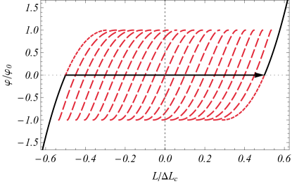
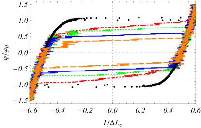
Figure 2: (Top) First order transition in the length for a quasi-static increase of the force. We use different colors for the stable parts of the branches (solid black) and the metastable parts (dashed red). The first branch $J=0$ is swept until the critical force $\varphi=0$ is reached. Then all the modules unfold simultaneously and the system goes directly to the completely unfolded branch $J=N=20$ (arrow). (Bottom) Hysteresis cycles under force-controlled conditions for a $N=20$ system. The lines correspond to simulations of the Langevin equations (6) for the temperature $T=0.02$ and different rates of variation of the force, namely $|dF/dt|=3\times 10^{-k}$, with $k=2$ (dot-dashed red), $k=3$ (dotted green), $k=4$ (solid blue), and $k=5$ (dashed orange). The same rates of variation of the force are considered for the very low temperature $T=2\times 10^{-5}$. All the curves are superimposed and thus they are plotted with the same symbols (black dots). For the higher temperature, the area of the hysteresis cycle decreases with the rate, approaching the behavior for a quasi-static process.

For a real, non-quasi-static process, the simple equilibrium picture above is not realized. Depending of the rate of variation of the force and the strength of the thermal fluctuations, the system will explore the metastable branches of the FEC. Then intermediate states between the completely folded and unfolded configurations will be seen hug10 ; rit06jpcm ; Ka12 ; pra12 . This is shown in the bottom panel of Fig. 2 by solving (6a)-(6b) with $k_{j}=\delta_{j}=0$ (in nondimensional form) for a 20-module protein, with $T=2\times 10^{-5}$ and $T=0.02$. All the $T=2\times 10^{-5}$ curves are superimposed on each other because the considered rates $|dF/dt|$ are small enough to lead to the adiabatic limit. For the upsweeping (downsweeping) process, the system moves over the completely folded (unfolded) branch until it reaches the end thereof, $\varphi=\varphi_{0}$ ($\varphi=-\varphi_{0}$). Then it jumps to the completely unfolded (folded) branch. The temperature is so small that the activated processes over the free energy barriers take place over a much longer time scale. For the higher temperature, $T=0.02$, the system can jump between the different minima of the potential and the force at which the system jumps between branches depends on the rate of variation of the force. Also, the system partially explores some of the intermediate branches. This picture is consistent: quite close to the adiabatic limit, the hysteresis cycle is large for the highest rate of variation, whereas the cycle shrinks towards the straight line $\varphi=0$ ($F_{c}=1$) as the rate tends to zero.

III.3 Length control

In length-controlled experiments, the length constraint introduces a long-range interaction between the protein modules. The equilibrium probability of any configuration $\bm{\eta}$ is now given by Eq. (15). Then the equilibrium configuration $\bm{\eta}^{\text{eq}}$ is found by minimizing $\mathit{A}$ with the constraint (2), and the difference between values of $\mathit{A}^{\text{eq}}$ at adjacent branches in the $F-L$ diagram governs the stability thereof. The length $\ell_{J}$ at which there is a change in the relative stability of two consecutive branches, with $J-1$ and $J$ unfolded units, is determined by the equality of their respective free energies $\mathit{A}^{\text{eq}}$. The corresponding forces $f_{J}^{-}\equiv F_{J-1}(\ell_{J})$ and $f_{J}^{+}=F_{J}(\ell_{J})$ over the branches with $J-1$ and $J$ unfolded units obey the system of two equations

$$\left.\mathit{A}_{J-1}^{\text{eq}}\right|_{f_{J}^{-}}\!=\left.\mathit{A}_{J}^{\text{eq}}\right|_{f_{J}^{+}},\quad\left.\mathit{L}_{J-1}^{\text{eq}}\right|_{f_{J}^{-}}\!=\left.\mathit{L}_{J}^{\text{eq}}\right|_{f_{J}^{+}}.$$ (27)

The force rips at $L=\ell_{J}$ are $N$ first-order equilibrium phase transitions because (i) the thermodynamic potential $\mathit{A}^{\text{eq}}$ is continuous at the transition, (ii) $F=(\partial\mathit{A}^{\text{eq}}/\partial L)_{Y}$ has a finite jump, from $f_{J}^{-}$ to $f_{J}^{+}<f_{J}^{-}$ at the $J$-th transition. In the top left panel of Fig. 3, we explicitly show $f_{1}^{-}$ and $f_{1}^{+}$. We have the following picture: As observed in Fig. 1, the branches $J-1$ and $J$ coexist on a certain range of lengths. Inside this range, Eq. (17) implies

$$\left(\frac{\partial}{\partial L}\left[\mathit{A}^{\text{eq}}_{J}-\mathit{A}^{\text{eq}}_{J-1}\right]\right)_{Y}=F_{J}(L)-F_{J-1}(L)<0,$$ (28)

where we have used (16). At equal length values $L$, the force is larger on the branch with a smaller number of folded units, $F_{J}(L)<F_{J-1}(L)$, $\forall J$. Therefore, $\mathit{A}^{\text{eq}}_{J-1}<\mathit{A}^{\text{eq}}_{J}$, and then the branch $J-1$ is the stable one and $J$ is metastable for $L<\ell_{J}$. The situation reverses for $L>\ell_{J}$, and there are not more stability changes between these branches because $\mathit{A}^{\text{eq}}_{J}-\mathit{A}^{\text{eq}}_{J-1}$ decreases monotonically as a function of $L$, as given by (28). Each intermediate branch ($J=1,\ldots,N-1$) is thus stable between $\ell_{J}$ and $\ell_{J+1}$, that is, between $f_{J}^{+}$ and $f_{J+1}^{-}$ (see top left panel of Fig. 3). A sawtooth pattern arises in the $F-L$ curve, with $N$ transitions between the $N+1$ branches at lengths $\ell_{1},\ldots,\ell_{N}$.

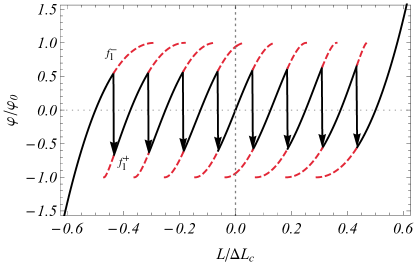
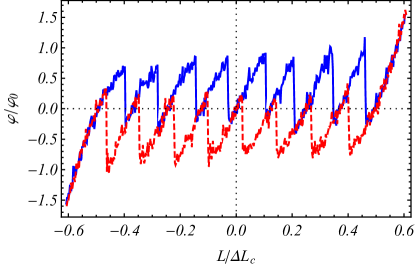
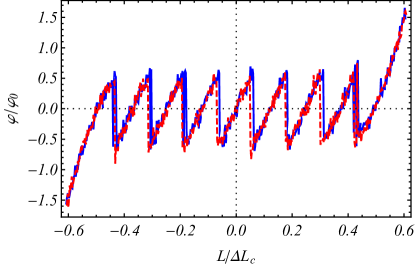
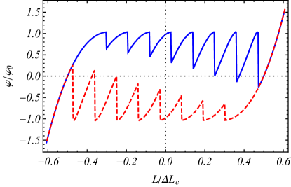
Figure 3: (Top left) Equilibrium force rips in the $F-L$ curve for a system with $N=8$ domains. We use different colors for the stable parts of the branches (solid black), metastable parts (dotted red), and the force rips (black arrows). The system follows the solid black curve in a quasi-static pulling process, with a series of first order transitions in the force (marked by the arrows). At the $J$-th transition, the force changes from $f_{J}^{-}$ (over the $(J-1)$th branch) to $f_{J}^{+}$ (over the $J$th branch). These forces $f_{J}^{\pm}$ increase with the number of unfolded units, as observed in AFM experiments with modular proteins, even though all the units are perfectly identical in the model. (Top right) Hysteresis cycle for a system composed of $N=8$ modules. The dimensionless temperature $T=0.02$, and the rate of variation of the length is $|dL/dt|=1.2\times 10^{-3}$ ($\dot{L}>0$, solid blue; $\dot{L}<0$, dashed red). (Bottom left) The same as in the top right panel, but for a smaller rate $|dL/dt|=1.2\times 10^{-6}$. Aside from thermal fluctuations, the system almost sweeps the equilibrium curve. (Bottom right) The same plot as in the bottom left panel, but for $T=2\times 10^{-5}$. Thermal fluctuations are so small that the system approaches the $T=0$ behavior, in which the branches are swept up to the end of the metastability region.

Similarly to the analysis for the force-controlled case, let us investigate the behavior of the system when the length is first increased and afterwards decreased with the same rate. Depending on the rate and the value of the temperature, a region of the metastable part of the branches is explored, and the force rips do not take place at the equilibrium values $\ell_{J}$. In Fig. 3, apart from the equilibrium force-extension curve (top left panel), we plot three unfolding/refolding cycles for an ideal 8-module protein. In the top right panel and the bottom left panels, the temperature is $T=0.02$ and the rates are $|dL/dt|=1.2\times 10^{-3}$ and $1.2\times 10^{-6}$, respectively. For the smallest rate, the system basically sweeps the equilibrium curve, aside from thermal fluctuations. Note that some of the transitions are “blurred” because of the hopping between the two posible forces at the transition length for this very small rate. On the other hand, for the highest rate, some hysteresis is present. Finally, in the bottom right panel, the temperature is much lower, $T=2\times 10^{-5}$, which results in the largest hysteresis cycle. This low temperature dynamical FEC is basically the same for the two rates considered before, $|dL/dt|=1.2\times 10^{-3}$ and $|dL/dt|=1.2\times 10^{-6}$, so only the latter is shown. The system sweeps each branch up to its limit of (meta)stability, $|\varphi/\varphi_{0}|=\pm 1$. Interestingly, this low temperature behavior resembles that of the chemical potential in a recent investigation of the thermodynamic origin of hysteresis in insertion batteries dre10 ; dre11 . This indicates that thermal fluctuations are less relevant for insertion batteries than for modular proteins, despite the similarities in their mathematical description. In our simulations, we have averaged the force over a unit time interval to mimic the experimental situation, in which the measuring devices have finite resolution footnote2 .

In the unfolding process, the transitions occur at forces/lengths that are displaced upward with respect to that of the refolding process, as usually observed in the experiments rit06jpcm ; lip01 ; hug10 ; OMCyF99 ; RPSyG99 ; SSHyR02 ; man05 ; lee10 . However, the unfolding/refolding curves for the simple Landau-like quartic potential we are using are much more symmetric than the experimental ones, reflecting the symmetry of the potential. In the experiments with modular proteins, the unfolding FEC exhibits large force rips similar to ours, but the refolding FEC does not present a sawtooth pattern OMCyF99 ; RPSyG99 ; SSHyR02 . Recently, however, several force rips have been observed in the refolding of the NI6C protein, both in AFM experiments and Steered Molecular Dynamics simulations lee10 . In Appendix A, we briefly analyze the predictions of our theory for the more realistic potential introduced in Ref. ber10 . In this case, the unfolding and refolding curves are strongly asymmetric and closely resemble the experimental ones.

For both, equilibrium and dynamical FECs (the latter being closer to the real experimental situation), (i) the size of the force rips decrease with the number of units $N$, and (ii) $f_{J}^{\pm}$ increase with the number of unfolded units $J$ for moderate values of $N$. The equilibrium case is illustrated by the top panel of Fig. 4. Interestingly, the increase with $J$ of the rips forces has been observed in modular proteins MyD12 ; fis00 ($N\sim 10$), whereas the rips forces are basically independent of $J$ for nucleic acids experiments (larger $N$) rit06jpcm ; hug10 ; HBFSByR10 . Also, it is worth noting that it has recently been shown that the length-controlled and the flow-controlled scenarios in polymer stretching are thermodynamically equivalent LHyS14 .

Let us investigate in more detail the dependence of the force rips size with the number of units $N$ in the equilibrium case; see left panels of Fig. 3. For large $N$, the free energy $\mathit{A}$ over each branch is extensive ($\propto N$), whereas the difference of free energies over consecutive branches for a given value of the length is independent of $N$. Therefore, the relative free energy change between consecutive branches scales as $N^{-1}$. Making use of Eq. (27) and neglecting terms of order $N^{-3}$, we obtain footnote3

$$\frac{f_{J}^{\pm}-F_{c}\!}{\varphi_{0}}=\mp\frac{3\sqrt{3}}{N}\!\left(1\mp\frac{r_{J}}{N}\right)\!,\quad r_{J}\!=\left.\frac{2\mathit{L}_{J}}{\mathit{L}_{N}-\mathit{L}_{0}}\right|_{F_{c}}\!.$$ (29)

Both $f_{J}^{-}$ and $f_{J}^{+}$ increase linearly with $J$, and so do $r_{J}$ and $\mathit{L}_{J}$, [$\mathit{L}_{J}$ is given by eq. (22b)]. This is necessary to fulfill the continuity condition for the free energy at the rips. On the other hand, for very large $N$, the term proportional to $r_{J}$ is proportional to $N^{-2}$ and, therefore, it is small compared with the first term on the rhs of eq.(29), which is proportional to $N^{-1}$. As a consequence, in this limit the force rips become independent of $J$ and symmetrical with respect to $F_{c}$,

$$\frac{f_{J}^{\pm}-F_{c}}{\varphi_{0}}\sim\mp\frac{3\sqrt{3}}{N}.$$ (30)

This is consistent with the behavior observed in nucleic acids rit06jpcm ; hug10 ; HBFSByR10 , in which the number of units is much larger than that typical of modular proteins. Moreover, it shows that the rip size in equilibrium follow a simple power law, it decays as $N^{-1}$ for large $N$. We show the tendency to this power law in the bottom panel of Fig. 4, in which we plot the size of the rip $\Delta F=f_{J}^{-}-f_{J}^{+}$ for a specific value of $J$. We have chosen $J=(M+1)/2$, that is, the transition in which the number of unfolded units become larger than the number of folded ones, $J$ increases from $(M-1)/2$ to $(M+1)/2$ ($M$ odd). Note that the fact that $\lim_{N\to\infty}f_{J}^{\pm}=F_{c}$ implies that all the units of the system unfold simultaneously at the critical force $F_{c}$ in the infinite size limit. This is the expected behavior, since in the thermodynamic limit as $N\to\infty$ force fluctuations disappear and the collectives with controlled force and controlled length should be utterly equivalent.

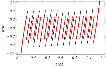
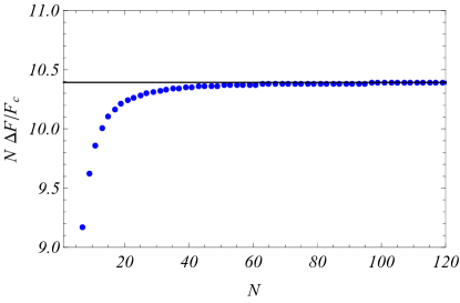
Figure 4: (Top panel) Zoom of the metastability region for two chains with $N=8$ (solid line) and $N=20$ (dashed line). The size of the rips decreases as the number of units $N$ increases, and it vanishes as $N\to\infty$. (Bottom panel) Decrease of the force rips with the number of units $N$. We plot the size of the rips $\Delta F=f_{J}^{-}-f_{J}^{+}$ for the “central” transition with $J=(M+1)/2$, scaled with the factor $N/F_{c}$ (circles). The limiting value $6\sqrt{3}$, which represents the power law behavior given Eq. (29), is shown with a solid line. It is observed that the system approaches rapidly this asymptotic behavior, being very close to it for $N\gtrsim 20$.

IV Chains with elastic interactions between identical modules

In this Section, we investigate the effect of the harmonic potential in Eq. (1) (proportional to $(\eta_{j}-\eta_{j-1})^{2}$), on the FECs. This term tends to minimize the number of “domain walls” separating regions with folded units from regions with unfolded units, as the domain walls give a positive contribution to the free energy that is proportional to their number. This elastic interaction is expected to be more relevant in experiments in which the unfolding/refolding of units is basically sequential, as in the case of unzipping/rezipping of DNA/RNA hairpins. The harmonic potential does not completely prevent the formation of “bubbles”, regions of unfolded units inside a domain of folded ones, but adds a free energy cost thereto. The same elastic interaction is responsible for the so-called depinning transition of wave fronts cb01 ; cba01 ; cb03 ; BT10 . The latter has been recently related to the experimentally observed stepwise unfolding of modular proteins under force-clamp conditions BCyP14 .

IV.1 Equilibrium states

First, we consider the case in which there is no disorder, all $k_{j}=k$ and $\delta_{j}=0$. The equilibrium extensions $\mathbf{\eta}^{\text{eq}}$ solve the minimization problem in Eqs. (11) or (16), that is,

$$a^{\prime}(\eta_{j}^{\text{eq}})-F+k(2\eta_{j}^{\text{eq}}-\eta_{j+1}^{\text{eq}}-\eta_{j-1}^{\text{eq}})=0,\quad j=1,\ldots,N.$$ (31)

These equations hold for all $j$, including the boundaries $1$, $N$, provided we introduce two fictitious extensions $\eta_{0}$, $\eta_{N+1}$, such that

$$\eta_{0}=\eta_{1},\quad\eta_{N+1}=\eta_{N}.$$ (32)

Alternatively, the extensions $\eta_{j}^{\text{eq}}$ can be regarded as the stationary solutions of the evolution equations (6a) with zero noise. Again, in the length-controlled case, $F$ is a Lagrange multiplier, calculated by imposing the constraint $L=\mathit{L}(\bm{\eta})$. The equilibrium extensions may be found by solving numerically (31), but they can also be built analytically by means of a perturbative expansion in powers of $k$, as we now show.

IV.1.1 Pinned wave fronts for $k\ll 1$

Substituting the expansion

$$\eta_{j}^{\text{eq}}=\sum_{n=0}^{\infty}\eta_{j,n}^{\text{eq}}k^{n},\quad j=1,\ldots,N,$$ (33)

into Eq. (31), we obtain

$$a^{\prime}(\eta_{j,0}^{\text{eq}})=F,$$ (34a)

$$\chi_{j}\eta_{j,1}^{\text{eq}}=\eta_{j+1,0}^{\text{eq}}+\eta_{j-1,0}^{\text{eq}}-2\eta_{j,0}^{\text{eq}},$$ (34b)

$$\chi_{j}\eta_{j,2}^{\text{eq}}=\eta_{j+1,1}^{\text{eq}}+\eta_{j-1,1}^{\text{eq}}-2\eta_{j,1}^{\text{eq}}-\frac{1}{2}\zeta_{j}(\eta_{j,1}^{\text{eq}})^{2},$$ (34c)

where

$$\chi_{j}=a^{\prime\prime}(\eta_{j,0}^{\text{eq}}),\quad\zeta_{j}=a^{\prime\prime\prime}(\eta_{j,0}^{\text{eq}}).$$ (35)

For $k=0$ we recover the results of the previous section, Eq. (34a) is the same as Eq. (19). The number of “unfolded” units $J$ having extensions $\eta^{(3)}$ determines the equilibrium values of Helmhotz free energy $\mathit{A}$, length $L$ and Gibbs free energy $\mathit{G}$ of the considered configuration, as given by eqs. (22a), (22b), and (25), respectively. There are $N!/[J!(N-J)!]$ configurations yielding the same values of $L$, $\mathit{A}$, and $\mathit{G}$ for $k=0$, a degeneracy that is partially broken at order $k$ by the elastic interaction. If three consecutive units $(j-1,j,j+1)$ are in the same potential well (either folded or unfolded) for $k=0$, then $\eta_{j,1}^{\text{eq}}=0$ and the stationary extension of the $j$-th unit does not vary. Therefore, only the modules at the domain walls separating domains where $\eta_{j}=\eta^{(1)}$ from others where $\eta_{j}=\eta^{(3)}$ change their extension. At the domain walls,

$$\eta_{j}^{\text{eq}}=\left\{\begin{array}[]{l}\eta^{(1)}+k\,\frac{\eta^{(3)}-\eta^{(1)}}{\chi^{(1)}}+\mathcal{O}(k^{2})\\ \eta^{(3)}-k\,\frac{\eta^{(3)}-\eta^{(1)}}{\chi^{(3)}}+\mathcal{O}(k^{2})\end{array}\right.$$ (36)

The length of the folded (unfolded) unit is slightly increased (decreased), as observed in Fig. 5 for $k=1.615$. Therein, the second-order corrections in $k$ are already very small. Thus, in the remainder of this section, we neglect $\mathcal{O}(k^{2})$ terms, that is, we write all the expressions up to the linear corrections in $k$. The equilibrium length and free energy for $J$ unfolded units and $M$ domain walls are,

$$\mathit{L}_{J,M}^{\text{eq}} = (N-J)\eta^{(1)}+J\eta^{(3)}$$ (37a)

$$+k\,M\frac{(\chi^{(3)}-\chi^{(1)})(\eta^{(3)}-\eta^{(1)})}{\chi^{(1)}\chi^{(3)}},$$

$$\mathit{G}_{J,M}^{\text{eq}} = (N-J)g^{(1)}+Jg^{(3)}+k\,\frac{M}{2}(\eta^{(3)}-\eta^{(1)})^{2}.$$

Thus, each domain wall contributes $k(\eta^{(3)}-\eta^{(1)})({\chi^{(1)}}^{-1}-{\chi^{(3)}}^{-1})$ to the length and $k(\eta^{(3)}-\eta^{(1)})^{2}/2$ to the free energy. An equivalent Ising model may be introduced to describe these equilibrium configurations, see Appendix B. The configurations with the fewest number of domain walls minimize the free energy $\mathit{G}$. For the boundary conditions (32), the minimal configurations have a single domain wall for a given value of the number of unfolded units $J$. The extension $\eta_{j}^{\text{eq}}$ increases with $j$ from $\eta^{(1)}$ to $\eta^{(3)}$, slowly across the sites inside either the folded and unfolded domains, and suddenly at the domain wall, see Fig. 5.

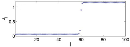
Figure 5: Stable stationary wave front with increasing profile from $u^{(1)}$ to $u^{(3)}$ (corresponding to $\eta^{(1)}$ and $\eta^{(3)}$, respectively) pinned at a particular point $j=J$ of an infinitely long chain, for $k=1.615$. The specular reflection of this pinned wave with respect to the center of the chain $j=N/2$ gives a pinned wave with decreasing profile from $\eta^{(3)}$ to $\eta^{(1)}$.

IV.1.2 Stability analysis

The pinned wave front solutions in Fig. 5 are stable in a certain range of forces, as proven in the literature cb01 ; cba01 ; cb03 ; BT10 . Here, we investigate the stability for small $k$, by looking at the second variation of the relevant thermodynamic potential. We have

$$\delta^{2}\mathit{G}=\delta^{2}\mathit{A}=\frac{1}{2}\sum_{j=1}^{N}a^{\prime\prime}(\eta_{j}^{\text{eq}})\,(\delta\eta_{j})^{2}+\frac{k}{2}\sum_{j=1}^{N+1}(\delta\eta_{j}-\delta\eta_{j-1})^{2},$$ (38)

where $\delta\eta_{j}=\eta_{j}-\eta_{j}^{\text{eq}}$. Note that the second variations of $A$ and $G$ are identical because the term proportional to $F$ does not contribute to $\delta^{2}\mathit{G}$. It must be stressed that the non-diagonal terms of the symmetric matrix corresponding to this quadratic form are of order $k$, namely $\partial^{2}\mathit{A}/\partial\eta_{j}\partial\eta_{j\pm 1}=\partial^{2}\mathit{G}/\partial\eta_{j}\partial\eta_{j\pm 1}=-k$, and they have not to be taken into account in our stability analysis.

Let us consider a domain of folded (unfolded) units, whose lengths are $\eta^{(1)}$ ($\eta^{(3)}$) for the ideal chain with $k=0$. Inside a domain of either folded or unfolded units, there is an additional positive contribution $2k$ to the diagonal terms $\partial^{2}\mathit{A}/\partial\eta_{j}^{2}$, so that stability is reinforced. Instability may arise at the domain walls, where

$$\frac{\partial^{2}\mathit{A}}{\partial\eta_{j}^{2}}=\chi^{(i)}+k\left[2-\frac{|\zeta^{(i)}|(\eta^{(3)}-\eta^{(1)})}{\chi^{(i)}}\right],\quad i=1,3.$$ (39)

Consistently with the notation introduced in Eq. (35), $\zeta^{(i)}=a^{\prime\prime\prime}(\eta^{(i)})=24\beta\eta^{(i)}$, $i=1,3$. Then $\zeta^{(1)}<0<\zeta^{(3)}$ because $\eta^{(1)}<0<\eta^{(3)}$. The first and last branch of the FEC correspond to all-folded and to all-unfolded modules, respectively. Their configurations do not involve domain walls and therefore $\partial^{2}\mathit{A}/\partial\eta_{j}^{2}=\chi^{(i)}$ for them, as in (39) with $k=0$. These branches are stable until $\chi^{(i)}=0$ at the extrema of $a^{\prime}(\eta^{\text{eq}})$. In contrast to this, the other FEC branches have configurations with one domain wall and the linear corrections in Eq. (39) cause $\partial^{2}\mathit{A}/\partial\eta_{j}^{2}$ to vanish for intermediate elongations between the extrema of $a^{\prime}(\eta^{\text{eq}})$. As the limit of stability of the FEC branches is given by the condition $\partial^{2}\mathit{A}/\partial\eta_{j}^{2}=0$, this reduces their size. This reduction in the branch size with $k$ is clearly observed in Fig. 6. We further illustrate this result in Fig. 7, where we plot the second derivatives of the on-site potential at the domain wall, both for $k=0$ and with the linear correction in $k$ (only for the folded unit at the domain wall, the curves for the unfolded unit are just the symmetrical ones with respect to $F_{c}=1$).

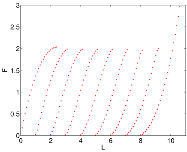
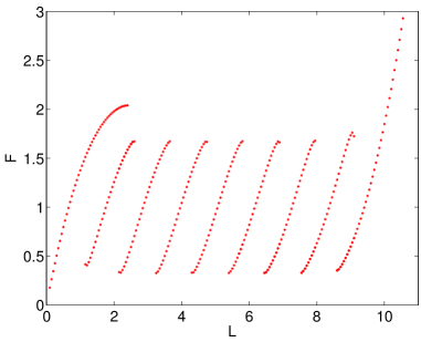
Figure 6: FECs for a system with $N=8$ modules. (Top) Stable stationary branches for $k=0.055$, quite similar to those for $k=0$ (see Fig. 1). (Bottom) Stable stationary branches, each corresponding to a wave front pinned at a different site $j=J$, $J=1,\ldots,8$, for $k=0.55$. The completely folded and unfolded branches are basically unchanged, but the size of the intermediate branches is considerably reduced. Here $L$ refers to the physical length (24b) that vanishes at $F=0$.

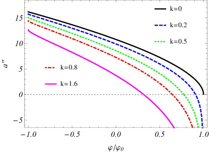
Figure 7: Second derivative of the potential for the folded unit at the domain wall up to order $k$, Eq. (39), as a function of the normalized force $\varphi/\varphi_{0}$. It is clearly seen that the stable part of the branch, with $a^{\prime\prime}>0$, decreases with $k$. For $k=0.5$ the size of the branch is reduced by $20\%$, approximately, from its maximum size ($k=0$), consistently with the behavior observed in Fig. 6.

IV.2 Deterministic dynamics

As the interacting chain is more complex than the ideal one, we start by neglecting thermal noise. This corresponds to the so-called deterministic (or macroscopic) approximation of the Langevin equation vK92 . Alternatively, this can be presented as solving the dynamical equations (6) at $T=0$. In a later Section, we will consider the changes introduced by a finite value of the temperature. Borrowing the usual terminology in classical mechanics, we refer to slow processes at $T=0$ as adiabatic, as they can no longer be regarded quasi-static because ergodicity is broken.

In Fig. 8, we plot two such processes. In the first one (top panel) we increase the length adiabatically in a stepwise manner, at each value of the length the system relaxes for a time $\Delta t$, after which the length is increased in $\Delta L$. We have chosen $\Delta L=0.2$ and $\Delta t=300$, for $k=0.5$. As compared to the equilibrium branches in Fig. 6, we observe that the $J$-th branch is swept as long it is locally stable, that is, until we reach the maximum value of the force $F_{J,\text{max}}$ at which $\delta^{2}\mathit{A}$ in (38) is no longer positive definite. Then the completely unfolded branch $J=0$ is swept to a higher force than all the intermediate branches: Its size is not reduced with respect to the $k=0$ case and $F_{0,\text{max}}>F_{J,\text{max}}$, $J=1,\ldots,N-1$, as discussed in Sec. IV.1.2. This means that the portion of the $J=1$ branch that is swept is smaller than all of the other intermediate branches ($J\neq 0,N$) and there appears a “bump” in the FEC at the transition point between the $J=0$ and $J=1$ branch. This is clearly observed in the top panel of Fig. 8 around the length corresponding to the transition from the $J=0$ to the $J=1$ branch, $L\simeq 2.4$. At this length, the corresponding force over the $J=1$ branch is much closer to the limit of stability of the intermediate branches than (for instance) the force over the $J=3$ branch at the transition length between the $J=2$ and $J=3$ branches ($L\simeq 3.7$). In the force-controlled case (bottom panel), we first increase the force adiabatically from $F=0$. The system moves over the branch of folded units, $J=0$, until it reaches the maximum thereof, $F_{0,\text{max}}$, at which the length jumps by $\Delta L=N[\eta^{(3)}(F_{0,\text{max}})-\eta^{(1)}(F_{0,\text{max}})]$ to the completely unfolded branch where $\eta_{j}=\eta^{(3)}(F_{\text{max}})$ for all $j$. If the force is now adiabatically decreased, the system moves over the branch of unfolded units, $J=N$, until the force reaches its minimum possible value and the system jumps back to the completely folded branch. Thus, for both length-controlled and force-controlled conditions, the largest possible hysteresis cycles appear, similar to the ones obtained in storage systems, see Fig. 5 of Ref. dre10 or Fig. 7 of Ref. dre11 .

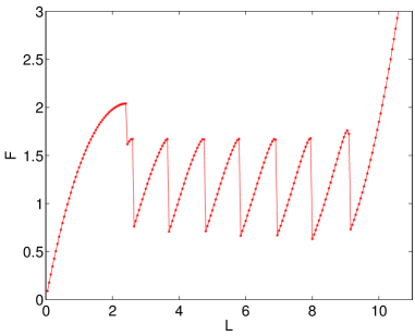
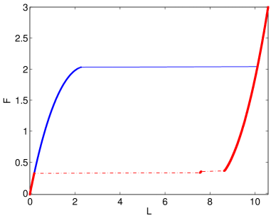
Figure 8: (Top) FEC obtained by adiabatically increasing the length of the system. The local maxima of the branches are close to the corresponding upper ends of the equilibrium branches in Fig. 6(b). (Bottom) Hysteresis loop obtained by adiabatic force sweeping the force–extension diagram of a chain of identical units at zero temperature. In both cases, $k=0.55$. $L$ is the physical length that vanishes at $F=0$, defined in Eq. (24b).

IV.3 Influence of quenched disorder

The biomolecules that are unfolded/refolded in the actual experiments, nucleic acids and proteins, are actually heteropolymers, as the units comprising a chain are not perfectly identical. This has led to investigate the effect of their intrinsic quenched disorder (or, equivalently, their intrinsic inhomogeneity) on their behavior in different physical situations BDyM98 ; GyT06 ; AyA07 . In the present context, their on-site double-well potentials $a(\eta_{j})$, their friction coefficients $\gamma_{j}$ and the spring constant between modules $k_{j}$ may depend on $j$. These considerations are much more important for DNA or RNA hairpins than for modular proteins. In the latter, the units in our mesoscopic picture are the modules, which have been artificially engineered to be as similar to each other as possible. In the equivalent experiment to find the current-voltage curves of superconductor superlattices, quenched disorder arises from fluctuations of the doping density at different wells GHMyP91 ; RTGyP02 . Including the natural variation in the free energy parameters amounts to adding quenched noises to them. To be concrete, we consider a potential whose strength depends on a random number $\delta_{j}$,

$$a^{\prime}(\eta_{j};\delta_{j})=(1+\delta_{j})a^{\prime}(\eta_{j},\delta_{j}=0).$$ (40)

which are i.i.d. random variables uniformly distributed on an interval $[-\beta,\beta]$ ($\beta<1$).

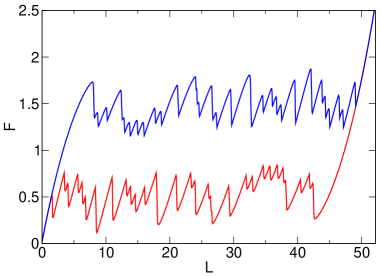
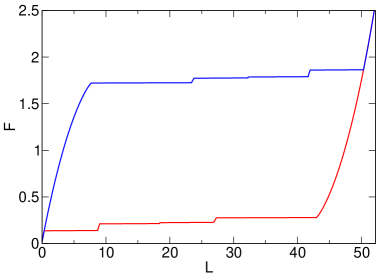
Figure 9: FEC for a DNA hairpin as in Figure 5 but with $N=40$ and disorder as in Eq. (40) (strength of the potential with $\beta=0.5$ and $k=1$). (Top) Hysteresis under length controlled conditions. The upper (lower) curve corresponds to adiabatically increasing (decreasing) length, with a rate $|dL/dt|=1.2\times 10^{-3}$ or smaller. (Bottom) Hysteresis under force-controlled conditions. Similarly, the upper (lower) curve corresponds to adiabatically increasing (decreasing) force, with a rate $|dF/dt|=3\times 10^{-3}$ or smaller. In the plots, $L$ is the physical length introduced in Eq. (24b).

Quenched disorder modifies both the stability of the FEC and the dynamics of the chain. When we depict the solutions corresponding to a wavefront pinned at particular locations as in Fig. 6, the presence of disorder moves the solution branches up and down and affects the dynamical behavior of the system. We show a hysteresis cycle under length-controlled conditions in the top panel of Figure 9. We have used a large disorder ($\beta=0.5$) which produces large variations in the length and height of the branches. Under force-controlled conditions, up and down sweeping the FEC, we obtain the much wider hysteresis cycles of the bottom panel of Fig. 9. Since the disorder changes the length and size of the force–extension branches, additional steps are seen in the hysteresis cycles, as compared to the case of identical units.

IV.4 Influence of thermal noise

In the last Section, we considered the effect of quenched disorder, but we still had zero temperature. Thermal noise allows random jumps between stable branches, provided the system has sufficient waiting time to escape the corresponding basins of attraction. As the control parameter (force or length) changes more slowly, the behavior of the system approaches the corresponding equilibrium statistical mechanics curve.

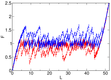
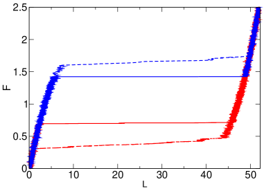
Figure 10: Same as in Fig. 9 but with additional white noise of temperature $T=0.02$. Thermal noise may suppress and blur solution branches. In both panels, the dashed curves correspond to the same rate as in Fig. 9, while in the solid ones the rate has been reduced by a factor $10^{-3}$. Again, $L$ is the physical length introduced in (24b).

Let us first consider length-controlled simulations. For an ideal biomolecule with identical modules, at $T=0$ adiabatic sweeping the FEC produces hysteresis cycles similar to the ones shown in Fig. 3 for a very low temperature. For finite temperature, (i) the size of the hysteresis cycles depends on the sweeping rate and becomes smaller as the rate decreases; (ii) there appear random jumps between stable branches that correspond to the same extension. Both effects have been observed in experiments with DNA hairpins, for which noise is much more important than in the case of modular proteins man05 ; lip01 ; lip02 ; hug10 . Also, some branches are not swept and the distinction between different branches is blurred, as shown in the top panel of Fig. 10. For a similar situation in semiconductor superlatices, see Fig. 2 in Ref. RTGyP02 , which shows a current-voltage curve for a sample comprising $40$ periods of $9$nm wide GaAs wells and $4$nm wide AlAs barriers. It is also interesting to note that there is always some “intrinsic” hysteresis in the last (first) rip of the FEC, even for the lowest rate for which a perfect reversible behavior was obtained in the ideal case. This behavior has been observed experimentally in the unzipping/rezipping of DNA, see Fig. 1C and Fig. S4 of Ref. HBFSByR10 , and also in superlattices, see Fig. 1 of Ref. GHMyP91 and Fig. 1 of Ref. BHGyT12 . As explained in Section IV.1.2, the FEC branch size is reduced in the non-ideal case ($k\neq 0$) except for the first and last branches whose configurations do not possess a domain wall. Then the non-zero interaction between neighboring modules makes the metastable regions in the first (completely folded) and the last (completely unfolded) branches wider than the rest.

In the force-controlled simulations, the effect of a finite temperature is shown in the bottom panel of Fig. 10. We observe a behavior similar to that in Fig. 2 for the ideal chain, and also to the one found in other models Ka12 ; pra12 . The physical picture is completely consistent with the experimental findings in nucleic acids hug10 .

V Final remarks

We have proposed a biomolecule model that includes an on-site quartic double-well potential and an elastic harmonic interaction among its modules in the free energy thereof. Despite its simplicity, it captures the main features of FECs in real biomolecules while allowing us to identify the main physical mechanisms and to keep a mathematically rigorous approach. This can be done in equilibrium but also for the dynamics, for which we have written the relevant Langevin (or Fokker-Planck equations). It should be stressed that the Fokker-Planck equation for the length-controlled case is not trivial, since the force $F$ appearing in the Langevin equation is an unknown that must be calculated by imposing the length constraint. The relevant thermodynamic potential, Gibbs-like (Helmholtz-like) for the force-controlled (length-controlled) case, has been shown to be the stationary solution of the Fokker-Planck equation.

Equilibrium FECs show multistability in a certain range of forces: There are multiple FEC branches corresponding to different number of folded/unfolded units. Under force-controlled conditions, there is an equilibrium phase transition between the all-modules-folded to the all-modules-unfolded, the lengths across the jump being determined by continuity of force and Gibbs free energy. Under length-controlled conditions, there appears a sawtooth FEC consisting of a number of branches with force jumps between them in which the number of unfolded modules differs by one. The forces across the jump are determined by continuity of length and Helmholtz free energy. In experiments, the unfolding/refolding transitions take place neither at a perfectly constant force nor at a perfectly constant length as seen in Figs. 2 and 3, because of the finite resolution of the the devices controlling the force or the length. Thus, the controlled quantity is not exactly equal to the desired value and also changes at the transition.

Dynamical FECs are obtained when the control parameter (either the force $F$ or the length $L$) is changed at a finite rate: Some hysteresis is present and the unfolding (refolding) forces increase (decrease) with the rate, as observed in experiments MNLRyE99 ; fis00 ; man05 ; lip01 ; lip02 ; fis00 ; hug10 ; CRJSTyB05 . A crucial role is played by the time that the system needs to surpass the energy barrier regulating the transitions from the folded to the unfolded state and viceversa. The key point is how this Arrhenius time scale compares to that defined by the variation of the force or length: It is only when the characteristic time defined by the variation of the force or length is longer than the Arrhenius time that the equilibrium FECs are recovered, because the force/length program can then be considered quasi-static and there is no hysteresis. We have shown in several cases throughout the paper that this feature implies that a decrease in the temperature (while keeping the rate of variation of the force/length) leads to a much wider hysteresis cycle. In this cycle, the system typically sweep the whole metastability region ($T=0$ or deterministic case).

Our results show that, in these elasticity experiments, biomolecules display what may be called a “metastable equilibrium behavior”. They follow stationary FEC branches that can be obtained out of the equilibrium solution of the Fokker-Planck equation, and dynamic out-of-equilibrium excursions do not depart too much from them. The hysteresis cycles, completely similar to those observed in real experiments, stem from equilibrium multistability: At the highest loading rates, the system is not able to reach the absolute minimum but sweeps a certain part of the metastable region (the narrower the smaller the rate is) of the equilibrium free energy landscape. There are techniques to obtain single molecule free energy differences from time-dependent driving about hysteresis cycles lip01 ; lip02 ; man05 ; CRJSTyB05 . In addition, the complete single molecule free energy landscape can be obtained using model-dependent algorithms HyS10 . Although there is some evidence of glass-like behavior in force-clamp experiments with proteins BHWyF06 , hysteresis in these unfolding/refolding experiments seems to be quite different from the more complex out-of-equilibrium hysteresis of glassy systems in cooling/heating cycles. When cooled down to low temperatures, glassy materials depart from the equilibrium curve and end up in a far from equilibrium state; when reheated, they return to equilibrium approaching a normal curve, which typically overshoots the equilibrium one ByP93 ; BPyR94 ; PByS97 ; RyS03 ; KGyC13 .

We have also discussed in detail the role of the interaction between neighboring units of the chain. The main effect of this interaction is the reduction of the width of the metastability region. When the elastic interaction is absent, all the configurations with the same number $J$ of unfolded units have the same free energy. This “entropic term” is reduced when the elastic interaction is taken into account, since the free energy also depends on the number of domain walls separating regions of unfolded and folded units and the configuration with only one domain wall (pinned wave front) is favored. From a physical point of view, this decrease is responsible for the reduction of force fluctuations, which are at the root of the width of the metastability region. Thus, we expect that the same behavior will be present for more realistic interaction potential between modules. In real biomolecules for which their on-site potentials and number of modules are similar, a smaller size of the rips may be linked to a stronger interaction between the neighboring units.

The relevance of the interaction between units is also clearly shown by the fact that the metastability regions in the first (completely folded) and last (completely unfolded) branches are wider than those of the intermediate ones. This leads to the existence of some “intrinsic” hysteresis in the first/last force rips of the FEC under length-controlled conditions, even for very low pulling rates, close to the quasi-static limit. Interestingly, this effect has been reported in experiments with DNA molecules, see for instance the FECs in Fig. 1C (rezipping) and Fig. S4 (unzipping) of Ref. HBFSByR10 . In the unzipping (rezipping) experiment, the physical reason is the “extra” free energy cost $k(\eta^{(3)}-\eta^{(1)})^{2}/2$ for creating (removing) the domain wall separating the folded and unfolded regions of the molecule. Thus, the presence or absence of intrinsic hysteresis may be used to discriminate the importance of the coupling between units in biomolecules or in other physical systems. For instance, compare Fig. 1 of BHGyT12 (or of GHMyP91 ) to Fig. 2 of RTGyP02 for the current-voltage curve obtained in the analogous experimental situation in semiconductor superlattices.

Many of the main characteristic behaviors observed here: multistability (multiple branches for a certain region of parameters like those in Fig. 1), the associated sawtooth FECs for length-controlled experiments, hysteresis effects when the control parameters are changed at a finite rate, etc. also occur in quite different physical situations, such as many particle storage systems dre10 ; dre11 ; dre11cmt and weakly coupled semiconductor superlattices GHMyP91 ; RTGyP02 ; BGr05 ; BT10 ; BHGyT12 . This analogy stems from the following common feature: all these systems comprise a number of similar bistable units whose individual states may be determined by a long-range interaction introduced by a global constraint (total charge dre10 ; dre11 ; dre11cmt , fixed voltage bias GHMyP91 ; RTGyP02 ; BGr05 ; BT10 ; BHGyT12 ). Of course, fine-detail differences appear in the observed behavior in each physical situation, depending on the relevance of non-ideal effects, such as interactions among modules, quenched disorder, or the thermal noise considered here. For instance, the maximum size hysteresis cycles, basically identical to the deterministic case, have been observed in Refs. dre10 ; dre11 for storage systems. This seems to indicate a lesser relevance of fluctuations in the latter.

Voltage biased semiconductor superlattices are definitely out-of-equilibrium systems: electrons are continuously injected and extracted from contacts, and their behaviors include time-periodic and chaotic oscillations besides hysteretic behavior BGr05 . Nonlinear charge transport in superlattices cannot be described with the free-energy scaffolding available for biomolecules. Instead, discrete drift-diffusion models based on sequential tunneling between neighboring quantum wells are used BGr05 ; BT10 . Nevertheless, the present paper shows that the methodology developed for these discrete systems can be adapted to describe FECs of biomolecules. As experiments with semiconductor superlattices are much more controllable than those with biomolecules, it would be interesting to see what the interpretation of measurements given in Refs. lip01 ; lip02 ; man05 ; CRJSTyB05 ; HyS10 produces in the superlattice case.

According to the above discussion, our main conclusions are quite general. They are applicable not only to biomolecules but to any physical system composed of repeated similar bistable units. Of course, we need renaming appropriately variables for each relevant physical situation. For instance, force-extension curves must be replaced by chemical potential-charge ones in storage systems dre10 ; dre11 or by current-voltage curves in semiconductor superlatices BGr05 ; BT10 . Depending on the system, some of the necessary experiments are not yet available. For instance, there are no precise current-controlled experiments on semiconductor superlattices. Thus our investigations open new interesting perspectives for experimental research in these fields.

Appendix A Asymmetric realistic potential

Here we consider the effects of using a more realistic free energy for the modules. This energy was first considered by Berkovich, Garcia-Manyes, Klafter, Urbakh and Fernandez (BGMKUF) to model the unfolding of single-unit proteins, such as I27 or ubiquitin, observed in AFM experiments ber10 . Very recently, we have employed it to investigate stepwise unfolding of polyproteins under force-clamp conditions BCyP14 . At zero force, the BGMKUF potential for one unit is

$$a(\eta) = U_{0}\!\left[\!\left(1-e^{-2b(\eta-R_{c})/R_{c}}\right)^{2}-1\right]\!$$ (41)

$$+\frac{k_{B}TL_{c}}{4P}\!\left(\frac{1}{1-\frac{\eta}{L_{c}}}-1-\frac{\eta}{L_{c}}+\frac{2\eta^{2}}{L_{c}^{2}}\right)\!.$$

This free energy for each unit is the sum of an enthalpic contribution given by a Morse potential and an entropic contribution given by a WLC potential, ber10 ; ber12 . Under application of force, the energy $A(x)-Fx$ exhibits two minima separated by a force-generated barrier ber10 . Manifestations of the sensitive dependance of unfolding and refolding on the barrier created by the applied force have been experimentally measured in elm12 ; bai12 . Here we use the parameter values of Ref. ber10 (slightly different from those in Ref. BCyP14 ), $P=0.4$nm (persistence length), $L_{c}=30$nm (contour length), $T=300$K, $U_{0}=100$pN nm($\sim\!\!24k_{B}T$), $R_{c}=4$nm, $b=2$. Force and extensions are measured in units of $[F]=100$ pN and $L_{c}=30$ nm, respectively. We define dimensionless variables, $\mu=U_{0}/(L_{c}[F])$, $\beta=2bL_{c}/R_{c}$, $\rho=R_{c}/L_{c}$, $A=k_{B}TL_{c}/(4PU_{0})$, thereby obtaining the following dimensionless potential

$$a(\eta) = \mu\!\left\{\left[1-e^{-\beta(\eta-\rho)}\right]^{2}-1\right.$$ (42)

$$\left.\quad+A\!\left(\frac{1}{1-\eta}-1-\eta+2\eta^{2}\right)\right\},$$

As repeatedly done throughout the paper, we keep the same notation for dimensionless and dimensional potentials. The dimensionless parameter values in (42) are $\mu=0.0333$, $\beta=30$, $\rho=0.133$, and $A=0.776$. On the other hand, the friction coefficient $\gamma$, given by the Einstein relation $D=k_{B}T/\gamma$, sets the time unit $[t]=\gamma L_{c}/[F]$. The diffusion coefficient for tethered proteins in solution $D$ has a typical value $D=1500$ nm²/s ber10 , so that $\gamma=0.00278$pN nm^-1s and $[t]=0.833$ms.

For this choice of parameters, there is metastability for forces in the range $F_{m}<F<F_{M}$, with $F_{m}=0.704$ ($7.04$pN) and $F_{M}=0.527$ ($52.7$pN). We show the equilibrium branches for two systems, with $N=8$ and $N=15$, respectively, in Fig. 11. Analogously to what we observed for the simple Landau-like free energy in Fig. 1, the branches become denser as the number of units increase. On the other hand, there is no up-down nor left-right symmetry: The branches are no longer symmetric with respect to either the critical force $F_{c}=15.6$pN, at which the folded and unfolded minima are equally deep, or the central branch with half of the units unfolded, $J=N/2$. Here, and throughout this Section, we have considered the “physical” length corresponding to the extension of the molecule with respect to its equilibrium length for zero force.

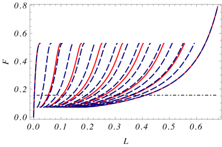
Figure 11: FECs for the BGMKUF potential, with $N=8$ (solid red) and $N=15$ (dashed blue). There are $N+1$ branches in the metastability region $F_{m}<F<F_{M}$, with the number of unfolded units $J$ increasing from left to right. The first ($J=0$) and last ($J=N$) branches are independent of $N$, as in Fig. 1. Note the asymmetry of the branches with respect to the critical force $F_{c}$ (dot-dashed line).

An unfolding/refolding cycle is shown in Fig. 12, in which the length $L$ is increased at a constant rate. We show the FEC corresponding to a typical AFM rate, namely $50$nm/s. In dimensionless variables, this means that $\dot{L}=0.0014$, because the unit of velocity is $L_{c}/[t]=3.6\times 10^{4}$nm/s. As for the Landau-like potential considered in the text, the force has been averaged over a certain time interval $\Delta t=1.2$ (corresponding to $1$ms) to mimic the finite resolution of the measuring devices in real experiments. Due to the asymmetry of the equilibrium branches, the unfolding and refolding curves are quite different, as seen in experiments. A clear sawtooth pattern is present in the unfolding curve: The molecule clearly sweeps a certain part of each equilibrium branch until it reaches a length at which it jumps to the neighboring branch. Similarly to experimental observations, this jump is associated to a decrease in the force (force rip) HyD12 ; MyD12 ; fis00 ; car99 . On the other hand, in the refolding process, the curve is much smoother and it is much more difficult to identify the intermediate branch that the system is sweeping, at least for the first stage of the relaxation curve (here, for $L\gtrsim 0.2$). This is analogous to the usual experimental behavior in the refolding process OMCyF99 ; RPSyG99 ; SSHyR02 . However, there appear clearer traces of force peaks in the refolding FEC when the molecule has partially relaxed ($L\lesssim 0.2$). This behavior resembles the FECs obtained for the NI6C protein in Ref. lee10 , see Figs. 1C, 1D, and S5 therein.

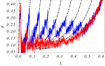
Figure 12: Unfolding/refolding cycle for a modular protein with $8$ units with free energies given by the BGMKUF potential. The dot-dashed lines correspond to the equilibrium branches of the FEC, see Fig. 11. There are sharp force rips in the unfolding process, each corresponding to the unfolding of one of the units (jumps between neighboring branches). In the refolding process, there are no sharp peaks until the length has almost completely relaxed, $L\lesssim 0.2$.

Although the previous unfolding/refolding cycle is very similar to those observed in experiments, it may be argued that our ideal length-control device may have some impact on the observed behavior. Therefore, we consider now a more realistic length-control device, as the one depicted in Fig. 1 of Ref. MyD12 , which leads to the length-control potential term in Eq. (5), where $\chi_{\text{lc}}$ is the (finite) spring constant of the cantilever. A typical value of the spring constant for an AFM experiment is $6$pN/nm, which gives a dimensionless value $\chi_{\text{lc}}=1.8$. Firstly, it is important to stress that the equilibrium branches of the FEC are not changed by the finite stiffness of the length-controlling device. The equilibrium extensions $\eta_{i}$ are given by Eq. (19), $a^{\prime}(\eta_{i})=F$, but now $F=-\chi_{\text{lc}}[L(\bm{\eta})-L]$ is the force exerted by the finite stiffness control device. Metastability appears in the same range of applied forces as in the case of ideal length control, the only difference is that the end to end distance $L(\bm{\eta})$ does not equal $L$, instead, $L(\bm{\eta})=L-F/\chi_{\text{lc}}<L$. In other words, the tip of cantilever has an equilibrium deflection $\Delta x=F/\xi_{\text{lc}}$ for each considered force $F$.

Repeating the unfolding/refolding process in Fig. 12, with the only difference of the finite value of the stiffness, we have obtained the results shown in Fig. 13. The unfolding/refolding cycles in both figures are very similar, although they would not match perfectly when superimposed. To obtain complete agreement with the perfect length control situation shown in Fig. 12, we should have employed a larger value of the spring constant, around $150$pN/nm or $\chi_{\text{lc}}=45$. In particular, the refolding curve is again much smoother than the unfolding sawtooth pattern found with either the quartic or the BGMKUF potential, but with some minor upward traces for $L\lesssim 0.2$.

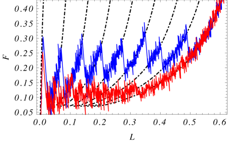
Figure 13: Unfolding/refolding cycle for a modular protein with $8$ units with free energies given by the BGMKUF potential and a finite value of the cantilever stiffness. The force $F$ is plotted against the end-to-end distance of the molecule $L=L(\bm{\eta})$. The equilibrium branches of the FEC, see Fig. 11, are the dot-dashed lines. Both the unfolding and refolding curves are very similar to those in Fig. 12, except for the force rips in the unfolding process not being perfectly vertical as a consequence of the imperfect length control.

Appendix B Equivalent Ising model for the free energy minima

We can write down the length and Gibbs free energy (37) in an Ising-like manner. Let us assign a spin-down variable to the folded units, so that $\sigma_{j}=-1$ if $\eta_{j,0}^{\text{eq}}=\eta^{(1)}$, and an spin-up $\sigma_{j}=+1$ to the unfolded ones, with $\eta_{j,0}^{\text{eq}}=\eta^{(3)}$. The number of unfolded units and domain walls are

$$J=\sum_{j=1}^{N}\frac{1+\sigma_{j}}{2},\qquad M=\sum_{j=1}^{N-1}\frac{1-\sigma_{j}\sigma_{j+1}}{2}.$$ (43)

Except for an additive constant, the free energy (LABEL:21.6b) becomes

$$\mathit{G}^{\text{eq}}(\bm{\sigma})=-H\sum_{j=1}^{N}\sigma_{j}-\Xi\sum_{j=1}^{N-1}\sigma_{j}\sigma_{j+1}+\mathcal{O}(k^{2}),$$ (44)

an Ising system with an external field $H$ and ferromagnetic nearest neighbor coupling $\Xi$ given by

$$H=\frac{g^{(3)}-g^{(1)}}{2},\quad\Xi=\frac{k[\eta^{(3)}-\eta^{(1)}]^{2}}{4}>0.$$ (45)

Interestingly, a similar expression for the free energy was proposed in Ref. makharov . The sign of $H$ determines which minimum of the Gibbs free energy $g(\eta)$ is deepest, $\eta^{(1)}$ or $\eta^{(3)}$; at the critical force $F_{c}=1$, that is, $H=0$, they are equally deep. The ferromagnetic coupling $\Xi\propto k$ favors the configurations with domains of parallel spins and thus a minimal number of domain walls for a given number of unfolded units $J$ note2 . Then $M=0$, when all the units are either folded or unfolded, or $M=1$, when there are both folded and undolded units, produce the minimum free energy (44).

Given (43), the length of the system at equilibrium is

$$\mathit{L}^{\text{eq}}(\bm{\sigma}) = \frac{N}{2}\left(\eta^{(1)}+\eta^{(3)}\right)+(N-1)\Delta$$ (46)

$$+\frac{\eta^{(3)}-\eta^{(1)}}{2}\sum_{j=1}^{N}\sigma_{j}-\Delta\sum_{j=1}^{N-1}\sigma_{j}\sigma_{j+1},$$

where

$$\Delta=\frac{k[\chi^{(3)}-\chi^{(1)}]}{2\chi^{(1)}\chi^{(3)}}.$$ (47)

The parameter $\Delta$ can be positive or negative. For the simple quartic potential we are considering, $\Delta=0$ at the critical force $F_{c}=1$, $\Delta>0$ for $F<F_{c}$, and $\Delta<0$ for $F>F_{c}$.

We have not considered here the quadratic corrections, proportional to $k^{2}$, which only affect sites at the domain walls and their nearest neighbors. In this equivalent Ising description, they (i) change the first order coupling constants $\Xi$ and $\Delta$, and (ii) introduce a second-nearest-neighbor interaction. Similarly, by taking into account higher order corrections, up to order $k^{n}$, we get an Ising model with longer-ranged interactions up to the $n$th-nearest-neighbors.

Appendix C Lyapunov function for the deterministic dynamics in the length-controlled case

Unlike the Gibbs free energy $\mathit{G}$ in the force-controlled case, the Helmholtz free energy $\mathit{A}$, as given by Eq. (1), is no longer a Lyapunov function of the zero-noise dynamics under length-controlled conditions with a known length dependence $L(t)$. However,

$$\tilde{\mathit{A}}(\bm{\eta}) = \mathit{A}(\bm{\eta})+\sum_{j=1}^{N}\!\Bigg{[}\frac{k}{2}(\eta_{j+1}-\eta_{j})^{2}$$

$$-\frac{\eta_{j}}{N}\!\left(\sum_{k=1}^{N}a^{\prime}(\eta_{k})+\frac{dL}{dt}\!\right)\!-\frac{a(\eta_{j})-\eta_{j}a^{\prime}(\eta_{j})}{N}\!\Bigg{]}\!.$$

is a Lyapunov function in this case. In fact, the governing nondimensional equations can be written as

$$\frac{d\eta_{j}}{dt}=-\frac{\partial}{\partial\eta_{j}}\tilde{\mathit{A}}(\bm{\eta}),$$ (49)

after eliminating $F$ by means of Eq. (7a). Then

$$\frac{d}{dt}\tilde{\mathit{A}}(\bm{\eta})=-\sum_{j=1}^{N}\!\left[\frac{\partial}{\partial\eta_{j}}\tilde{\mathit{A}}(\bm{\eta})\right]^{2}\!\leq 0.$$

Also,

$$\tilde{\mathit{A}}(\bm{\eta})>N\min_{u}\!\left[a(u)-Fu-\frac{a(u)-ua^{\prime}(u)}{N}\right]\!$$

for

$$F_{m}<F=\frac{1}{N}\sum_{j=1}^{N}a^{\prime}(\eta_{j})+\frac{1}{N}\frac{dL}{dt}<F_{M}.$$

References

- (1) F. Ritort, J. Phys.: Condens. Matter 18, R531-R583 (2006).
- (2) S. Kumar and M. S. Li, Phys. Rep. 486, 1 (2010).
- (3) P. E. Marszalek and Y. F. Dufrêne, Chem. Soc. Rev. 41, 3523 (2012).
- (4) S. B. Smith, Y. Cui and C. Bustamante, Science 271, 795-799 (1996).
- (5) M. Carrion-Vázquez, A. F. Oberhauser, S. B. Fowler, P. E. Marszalek, S. E. Broedel, J. Clarke and J. M. Fernandez, Proc. Natl. Acad. Sci. USA 96, 3694-3699 (1999).
- (6) H. Lu and K. Schulten, Proteins Struct. Funct. Genet. 35, 453-463 (1999).
- (7) T. E. Fisher, P. E. Marszalek and J. M. Fernandez, Nature Struct. Biol. 7, 719-724 (2000).
- (8) J. Liphardt, B. Onoa, S. B. Smith, I. Tinoco and C. Bustamante, Science 292, 733-737 (2001).
- (9) C. Bustamante, Z. Bryant and S. B. Smith, Nature 421, 423-427 (2003).
- (10) M. Manosas and F. Ritort, Biophys. J. 88, 3224-3242 (2005).
- (11) Y. Cao, R. Kuske and H. Li, Biophys. J. 95, 782-788 (2008).
- (12) Thus, the total length should not be confused with the contour length of the biomolecule, which is a fixed quantity.
- (13) J. Liphardt, S. Dumont, S. B. Smith, I. Tinoco, and C. Bustamante, Science 296, 1832-1835 (2002).
- (14) J. M. Huguet, Statistical and thermodynamic properties of DNA unzipping experiments with optical tweezers. Ph.D. Thesis, Universitat de Barcelona, 2010.
- (15) C. Bustamante, J. F. Marko, E. D. Siggia, and S. Smith, Science 265, 1599-1600 (1994).
- (16) J. F. Marko and E. D. Siggia, Macromolecules 28, 8759-8770 (1995).
- (17) R. Berkovich, S. Garcia-Manyes, J. Klafter, M. Urbakh, and J. M. Fernandez, Biophysical J. 98, 2692-2701 (2010); Biochem. and Biophys. Reasearch Comm. 403, 133-137 (2010).
- (18) R. Berkovich, R. I. Hermans, I. Popa, G. Stirnemann, S. Garcia-Manyes, B. J. Bernes, and J. M. Fernandez, Proc. Nat. Acad. Sci. 109, 14416-14421 (2012).
- (19) D. Keller, D. Swigon, and C. Bustamante, Biophys. J. 84, 733 (2003).
- (20) J. M. Rubí, D. Bedeaux, and S. Kjelstrup, J. Phys. Chem. 110, 12733 (2006).
- (21) A. Prados, A. Carpio, and L. L. Bonilla, Phys. Rev. E 88, 012704 (2013).
- (22) J. M. Huguet, C. V. Bizarro, N. Forns, S. B. Smith, C. Bustamante, and F. Ritort, Proc. Natl. Acad. Sci. 107, 15431 (2010).
- (23) D. Reguera, J. M. Rubí, and J. M. G. Vilar, J. Phys. Chem. 109, 21502 (2005).
- (24) S. Park, F. Khalili-Araghi, E. Tajkhorshid, and K. Schulten, J. Chem. Phys. 119, 3559 (2003)
- (25) D. Collin, F.Ritort, C. Jarzynski, S. B. Smith, I. Tinoco Jr., and C. Bustamante, Nature 437, 231 (2005).
- (26) G. Hummer and A. Szabo, Proc. Nat. Acad. Sci. 107, 21441 (2010).
- (27) A. Prados, A. Carpio and L. L. Bonilla, Phys. Rev. E 86, 021919 (2012).
- (28) L. L. Bonilla, A. Carpio, and A. Prados, EPL 108, 28002 (2014).
- (29) W. Dreyer, J. Jamnik, C. Guhlke, R. Huth, and M. Gaberscek, Nature Mater. 9, 448-453 (2010).
- (30) W. Dreyer, C. Guhlke, and R. Huth, Physica D 240, 1008-1019 (2011).
- (31) W. Dreyer, C. Guhlke, and M. Herrmann, Continuum Mech. Thermodyn. 23, 211-231 (2011).
- (32) H. T. Grahn, R. Haug, W. Muller, and K. Ploog, Phys. Rev. Lett. 67, 1618 (1991).
- (33) M. Rogozia, S. W. Teitsworth, H. T. Grahn, and K. H. Ploog, Phys. Rev. B, 65, 205303 (2002).
- (34) L. L. Bonilla and H. T. Grahn, Rep. Prog. Phys. 68, 577-683 (2005).
- (35) L. L. Bonilla and S. W. Teitsworth, Nonlinear wave methods for charge transport, (Wiley-VCH, Weinheim, 2010).
- (36) Yu. Bomze, R. Hey, H.T. Grahn and S.W. Teitsworth, Phys. Rev. Lett. 109, 026801 (2012).
- (37) T. Hoffmann and L. Dougan, Chem. Soc. Rev. 41, 4781-4796 (2012).
- (38) N. Forns, S. de Lorenzo, M. Manosas, K. Hayashi, J. M. Huguet, and F. Ritort, Biophys. J. 100 1765 (2011).
- (39) A. F. Oberhauser, P. K. Hansma, M. Carrion-Vazquez, and J. M. Fernandez, Proc. Nat. Acad. Sci. 98, 46468 (2001).
- (40) J. M. Fernandez and H. Li, Science 303, 1674 (2004).
- (41) G. Hummer and A. Szabo, Biophys. J. 85, 5 (2003).
- (42) The length is extensive in the sense that it is proportional to the number of units in the limit as .
- (43) C. J. Thompson, Classical equilibrium statistical mechanics, (Oxford U.P., Oxford, 1988).
- (44) V. Y. Chernyak, M. Chertkov, and C. Jarzynski, J. Stat. Mech: Theor. Exp. P08001 (2006).
- (45) L. D. Landau and E. M. Lifshitz, Statistical Physics Part 1 (Course of Theoretical Physics, vol. 5), (Pergamon Press, Oxford, 1980).
- (46) In biomolecules at zero force, the folded state is much more localized than the unfolded state but this feature cannot be reproduced with the simple Landau-like potential we are using. Due to its simplicity, the barrier separating the two minima is always closer to the metastable state. In order to make the “width” of the folded state smaller than that of the unfolded state, more realistic potentials like the one in Refs. ber10 ; ber12 ; BCyP14 must be used.
- (47) R. Kapri, Phys. Rev. E 86, 041906 (2012).
- (48) This time interval is much longer than the time step used to integrate the Langevin equations, but much shorter than the total time for the stretching (or relaxing) process. As a result, the plotted force is close to , Eq. (8b), because the time average of is very small.
- (49) A. F. Oberhauser, P. E. Marszalek, M. Carrion-Vazquez and Julio M. Fernandez, Nature Struct. Biol. 6, 1025 (1999).
- (50) M. Rief, J. Pascual, M. Saraste, and H. E. Gaub, J. Mol. Biol. 286, 553 (1999).
- (51) I. Schwaiger, C. Sattler, D. R. Hostetter, and M. Rief, Nature Materials 1, 232 (2002).
- (52) W. Lee, X. Zeng, H.-X. Zhou, V. Bennet, W. Yang, and P. E. Marszalek, J. Biol. Chem. 285, 38167 (2010).
- (53) F. Latinwo, K.-W. Hsiao, and C. M. Schroeder, J. Chem. Phys. 141, 174903 (2014).
- (54) In Ref. pra13 , it was instead of in the numerator of . Equation (29) is more consistent, since is of the order of .
- (55) A. Carpio and L. L. Bonilla, Phys. Rev. Lett. 86, 6034-6037 (2001).
- (56) A. Carpio, L.L. Bonilla and G. Dell’Acqua, Phys. Rev. E 64, 036204 (2001).
- (57) A. Carpio and L. L. Bonilla, SIAM J. Appl. Math. 63, 1056-1082 (2003).
- (58) N. G. van Kampen, Stochastic Processes in Physics and Chemistry (North-Holland, Amsterdam, 1997).
- (59) D. Bensimon, D. Dohmi, and M. Mézard, Europhys. Lett. 42, 97 (1998).
- (60) G. Giacomin and F. L. Toninelli, Phys. Rev. Lett. 96, 070602 (2006).
- (61) S. Ares and A. Sánchez, Eur. Phys. J. B 56, 253–258 (2007).
- (62) R. Merkel, P. Nassoy, A. Leung, K. Ritchie, and E. Evans, Nature 397, 6714 (1999).
- (63) J. Brujić, R. I. Hermans, K. A. Walther, and J. M. Fernandez, Nature Phys. 2, 282 (2006).
- (64) J. J. Brey and A. Prados, Phys. Rev. E 47, 1541 (1993).
- (65) J. J. Brey and A. Prados, Phys. Rev. B 49, 984 (2004); J. J.Brey, A. Prados and M. J. Ruiz-Montero, J. Non-Cryst. Solids 172-174, 371 (1994).
- (66) A. Prados, J. J. Brey, and B. Sánchez-Rey, Phys. Rev. B 55, 6343 (1997); A. Prados and J. J. Brey, Phys. Rev. E 64, 041505 (2001).
- (67) F. Ritort and P. Sollich, Adv. Phys. 52, 219 (2003).
- (68) A. S. Keysa, J. P. Garrahan, and D. Chandler, Proc. Nat. Acad. Sci. 110, 4482 (2013).
- (69) P. J. Elms, J. D. Chodera, C. Bustamante and S. Marqusee, Proc. Nat. Acad. Sci. 109, 3796 (2012).
- (70) H. Bai, J. E. Kath, F. M. Zörgiebel, M. Sun, P. Ghosh, G. F. Hatfull, N. D. F. Grindley, and J. F. Marko, Proc. Nat. Acad. Sci. 109, 16546 (2012).
- (71) D. E. Makharov, Biophys. J. 96, 2160 (2009).
- (72) The boundary conditions (32) imply that the terms corresponding to and do not contribute to the interaction between nearest neighbor spins.