COMPARING DENSE GALAXY CLUSTER REDSHIFT SURVEYS WITH WEAK LENSING MAPS

Abstract

We use dense redshift surveys of nine galaxy clusters at $z\sim 0.2$ to compare the galaxy distribution in each system with the projected matter distribution from weak lensing. By combining 2087 new MMT/Hectospec redshifts and the data in the literature, we construct spectroscopic samples within the region of weak-lensing maps of high (70–89%) and uniform completeness. With these dense redshift surveys, we construct galaxy number density maps using several galaxy subsamples. The shape of the main cluster concentration in the weak-lensing maps is similar to the global morphology of the number density maps based on cluster members alone, mainly dominated by red members. We cross correlate the galaxy number density maps with the weak-lensing maps. The cross correlation signal when we include foreground and background galaxies at 0.5$z_{\rm cl}<z<2z_{\rm cl}$ is $10-23$% larger than for cluster members alone at the cluster virial radius. The excess can be as high as 30% depending on the cluster. Cross correlating the galaxy number density and weak-lensing maps suggests that superimposed structures close to the cluster in redshift space contribute more significantly to the excess cross correlation signal than unrelated large-scale structure along the line of sight. Interestingly, the weak-lensing mass profiles are not well constrained for the clusters with the largest cross correlation signal excesses ($>$20% for A383, A689 and A750). The fractional excess in the cross correlation signal including foreground and background structures could be a useful proxy for assessing the reliability of weak-lensing cluster mass estimates.

1. INTRODUCTION

Measurement of the mass distribution in galaxy clusters is an important test of structure formation models (Duffy et al., 2008; Prada et al., 2012; Rines et al., 2013). Among the many measurements of the mass distribution of clusters, only weak lensing (e.g., Hoekstra 2007; Okabe & Umetsu 2008; Okabe et al. 2010; Umetsu et al. 2014) and the caustic method based on galaxy kinematics (Diaferio & Geller, 1997; Diaferio, 1999; Serra et al., 2011) reliably measure the cluster mass distribution regardless of the cluster dynamical state. These measures can both extend into the infall region (Geller et al., 2013).

Weak-lensing has grown into a powerful probe of the distribution of dark matter because it measures the total mass of a system directly regardless of the baryon content and/or dynamical state (Clowe et al., 2006; Huterer, 2010; Shan et al., 2012). However, weak lensing includes the effect of structures projected along the line of sight (Hoekstra, 2001); lensing provides a map of the total projected surface mass density. There are also several unresolved systematic errors in weak-lensing analysis: e.g., systematic uncertainties in the measurements of gravitational shear and in the photometric redshift estimation of the distribution of lensed sources (Huterer et al., 2013; Utsumi et al., 2014).

The signal in weak-lensing maps centered on a cluster is generally dominated by the cluster itself. However, there is an expected contribution to the signal from large-scale structure either associated or not associated with the cluster (Hoekstra, 2001, 2003; Dodelson, 2004). These structures are sometimes resolved in the weak-lensing maps, and can often appear even within the virial radii of clusters. The lensing signal from these structures may introduce a bias and/or increase the uncertainty in a cluster mass estimate based on lensing (Hoekstra et al., 2011b; Becker & Kravtsov, 2011; Gruen et al., 2011; Bahé et al., 2012; Coe et al., 2012).

Galaxy redshift surveys provide a map of the three-dimensional galaxy distribution. They can thus be used to resolve the structures along the line of sight that may contribute to the total projected mass (Hoekstra et al., 2011a; Geller et al., 2010, 2013, 2014b). Use of redshift surveys can also mitigate systematic errors resulting from the use of photometric redshifts in weak-lensing analysis (Coupon et al., 2013). A direct comparison of the structures identified in weak-lensing maps and in redshift surveys provides an important test of the issues limiting applications of weak lensing to measurement of cluster masses and mass profiles, and to the identification of galaxy clusters (Geller et al., 2005, 2010; Kurtz et al., 2012; Utsumi et al., 2014; Starikova et al., 2014).

Table 1List of Galaxy Clusters

Name	R.A.2000	Decl.2000	z	Source of	Number of	Completeness	Subaru	Radius of	Number of
	(deg)	(deg)		redshifts	$z$ inside	inside	FOV	entire field	of $z$ for
					Subaru FOV	Subaru FOV	(arcmin)	(arcmin)	entire field
A383	42.01417	$-$3.52914	0.1887	1	411/153	82%	20${}^{\prime}\times$20′	51	2544/275
A267	28.17485	1.00709	0.2291	2	419/154	76%	20${}^{\prime}\times$20′	33	1611/192
A611	120.23675	36.05654	0.2880	3,4	335/129	76%	20${}^{\prime}\times$20′	37	1836/295
A689	129.35600	14.98300	0.2789	2,5	333/119	73%	20${}^{\prime}\times$20′	33	1282/220
A697	130.73982	36.36646	0.2812	2,5,6	284/149	89%	16${}^{\prime}\times$16′	33	1152/269
A750	137.24690	11.04440	0.1640	2,5	540/211	73%	24${}^{\prime}\times$24′	33	1344/305
A963	154.26513	39.04705	0.2041	2,5,7	318/161	70%	18${}^{\prime}\times$18′	33	1516/379
RXJ1720.1+2638	260.04183	26.62557	0.1604	2,8	220/121	89%	14${}^{\prime}\times$14′	33	1511/349
RXJ2129.6+0005	322.41647	0.08921	0.2339	2,9	156/71	71%	12${}^{\prime}\times$12′	41	3522/249

Table 2Redshifts in the fields of A689, A697, A750 and A963

Cluster	ID	SDSS ObjID	R.A.2000	Decl.2000	$m_{\rm r,Petro,0}$	$z$	$z$	Member
		(DR10)	(deg)	(deg)	(mag)		Source
A689	1	1237667291574042910	128.795409	14.957459	18.939	$0.00011\pm 0.00003$	3	0
A689	2	1237667538535055415	128.801168	15.053992	20.484	$0.52506\pm 0.00018$	3	0
A689	3	1237667538535055402	128.802527	15.004511	17.237	$0.00009\pm 0.00001$	3	0
A689	4	1237667538535055664	128.808520	15.046711	17.286	$0.13889\pm 0.00003$	3	0
A689	5	1237667291574042897	128.812113	14.875166	17.978	$0.00021\pm 0.00001$	3	0
A689	6	1237667538535055646	128.816686	15.004262	19.290	$-0.00004\pm 0.00005$	3	0
A689	7	1237667291574042924	128.825021	14.912634	17.442	$0.15485\pm 0.00003$	3	0
A689	8	1237667538535055723	128.827412	15.141970	17.646	$0.15470\pm 0.00004$	3	0
A689	9	1237667538535055734	128.830726	15.171179	17.600	$0.16997\pm 0.00003$	3	0
A689	10	1237667291574042958	128.839568	14.954218	17.674	$0.00081\pm 0.00001$	3	0

As an example of the impact of superimposed structure on a weak-lensing map, Geller et al. (2014a) used a deep, dense, nearly complete redshift survey of the strong lensing cluster A383 to compare the galaxy distribution with the weak-lensing results of Okabe et al. (2010). The weak-lensing map of A383 matches the galaxy number density map based on cluster members alone very well. However, a secondary peak in the weak-lensing map is not clearly visible in the galaxy number density map based on members (see their Fig. 8). A galaxy number density map that includes foreground and background galaxies around A383 produces a secondary peak consistent with the secondary weak lensing peak. Thus, the secondary lensing peak apparently results from a superposition of foreground and background structures around A383. The secondary peak lies within the virial radius of A383 and the cluster mass profile can be affected by superimposed structures even within the virial radius. The pilot study of A383 demonstrates the importance of dense redshift surveys to understand the projected mass distribution revealed by weak lensing.

Here, we compare maps based on dense redshift surveys with weak-lensing maps for nine additional clusters. We compare the structures identified in the galaxy number density and weak-lensing maps by cross correlating the two. With this sample we begin to quantify and elucidate the contribution to weak-lensing maps from structures superimposed along the line of sight.

Section 2 describes the cluster sample and the data including the weak-lensing maps and the deep redshift surveys. We measured 2087 new redshifts to obtain galaxy number density maps uniformly complete to $m_{r}=20.5$ for each cluster. We compare galaxy number density maps of galaxy clusters with the corresponding weak-lensing maps in Section 3. We discuss the results and conclude in Sections 4 and 5, respectively. Throughout, we adopt flat $\Lambda$CDM cosmological parameters: $H_{0}=100h$ km s^-1 Mpc^-1, $\Omega_{\Lambda}=0.7$ and $\Omega_{m}=0.3$.

2. DATA

Among the 30 clusters at $z\sim 0.2$ with high-quality Subaru weak-lensing maps in Okabe et al. (2010), we select nine galaxy clusters with nearly complete redshift survey data. With the inclusion of redshifts measured in this study, all nine clusters have an overall spectroscopic completeness within the region of weak-lensing map $>70\%$ for $m_{\rm r,Petro,0}\leq 20.5$.

Table 1 lists the nine clusters with the redshift source, the number of redshifts and the overall spectroscopic completeness within the weak-lensing maps, the field-of-views (FOVs) of the weak-lensing maps, the size of the entire cluster field where we compile the redshift data, and the number of redshifts in the entire field. Here we describe the data we use to compare the redshift surveys with the weak lensing results.

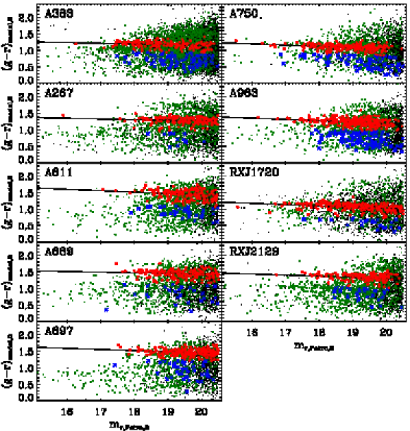
Figure 1.— Color-magnitude diagram for galaxies in the fields of nine galaxy clusters. Black dots and green squares are galaxies without and with spectroscopic redshifts, respectively. Red circles and blue crosses are red and blue member galaxies with spectroscopic redshifts, respectively. Solid line is the best-fit of the red sequence in each cluster.

2.1. Weak-Lensing Maps

Okabe et al. (2010) use Subaru/Suprime-Cam images (Miyazaki et al., 2002) for 30 X-ray luminous galaxy clusters at $0.15\leq z\leq 0.3$ to determine the mass distribution around clusters. Their paper includes a two-dimensional weak-lensing map of each cluster field. The map provides the normalized mass density field (i.e., the lensing convergence field, $\kappa$) relative to the 1$\sigma$ noise level expected from the intrinsic ellipticity noise. These maps are the basis for their derivation of projected mass distribution around each cluster.

Typical FOVs of the maps are $20^{\prime}\times 20^{\prime}$. They smooth the map with the Gaussian, typical FWHM of $1^{\prime}.2$. The range of FWHM is $1^{\prime}.0-1^{\prime}.7$. We adopt their maps, listed in their Figures 16–45 (see their Appendix 3 for more details about the construction of the maps). Among the 30 clusters in their sample, we selected nine clusters where we measured new redshifts as necessary.

2.2. The Cluster Redshift Surveys

To compare the galaxy number density and weak-lensing map of a cluster, it is necessary to have a sufficiently dense, nearly complete redshift survey of the cluster (e.g., Geller et al. 2014a). Among the 30 clusters at $z\sim 0.2$ with Subaru weak-lensing maps in Okabe et al. (2010), we first select five clusters with dense redshift data in the Hectospec Cluster Survey (HeCS, Rines et al. 2013). We supplement these data with redshifts from the literature (Girardi et al., 2006; Drinkwater et al., 2010; Owers et al., 2011; Lemze et al., 2013; Jaffé et al., 2013; Geller et al., 2014a), the Sloan Digital Sky Survey data release 10 (SDSS DR10, Ahn et al. 2014), and the NASA/IPAC Extragalactic Database (NED).

HeCS primarily observed galaxies close to the red sequence; because our goal here is to study all line-of-sight structure in the FOVs of the clusters, we require additional observations to obtain magnitude-limited redshift surveys. We made additional observations of four HeCS clusters (A689, A697, A750 and A963) in 2013 February and March with the 300 fiber Hectospec on the MMT 6.5m telescope (Fabricant et al., 2005). The four clusters are within the footprint of the SDSS DR10. To obtain a high, uniform spectroscopic completeness at $m_{\rm r,Petro,0}\leq 20.5$ within the field of the weak-lensing map, we weighted the spectroscopic targets according to the galaxy apparent magnitude independent of color.

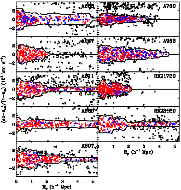
Figure 2.— Redshift (rest-frame clustercentric velocity) diagram for the nine clusters in this study. Red circles and blue crosses are red and blue member galaxies, respectively. Open circles are non-member galaxies. Black lines are the caustics that distinguish member and non-member galaxies.

We used the 270 line mm^-1 grating of Hectospec that provides a dispersion of 1.2 Å pixel^-1 and a resolution of $\sim$6 Å. We used 3$\times$20 minute exposures for each field, and obtained spectra covering the wavelength range $3650-9150$ Å. During the pipeline processing, spectral fits are assigned a quality flag of “Q” for high-quality redshifts, “?” for marginal cases, and “X” for poor fits. We use only the spectra with reliable redshift measurement (i.e. “Q”). We set up two or three different Hectospec fields for each cluster, and obtained 470–610 reliable redshifts per cluster.

Table 2 lists the galaxy redshift data in the fields of the clusters. We list 5294 galaxies with measured redshifts including 2087 new Hectospec redshifts for four clusters (A689, A697, A750 and A963). The table contains the cluster name, identification, SDSS DR10 ObjID, the right ascension (R.A.), declination (Decl.), $r$-band Petrosian magnitude with Galactic extinction correction (from the SDSS DR10), the redshift ($z$) and its error, the redshift source, and the cluster membership flag.

Figure 1 shows Galactic extinction corrected (denoted by the subscript, “0”) $(g-r)_{\rm model,0}-m_{\rm r,Petro,0}$ color-magnitude diagram for each cluster. Black dots and green squares are extended sources without and with measured redshifts, respectively. Red circles and blue crosses are red and blue cluster member galaxies. Obviously, most bright galaxies have measured redshifts. The plot includes all the sources in the entire cluster field (see Table 1 for the field size) including the galaxies outside the weak-lensing maps, thus there are some bright galaxies without measured redshifts. We explain the details of the spectroscopic completeness in the region covered by each weak-lensing map in the next section.

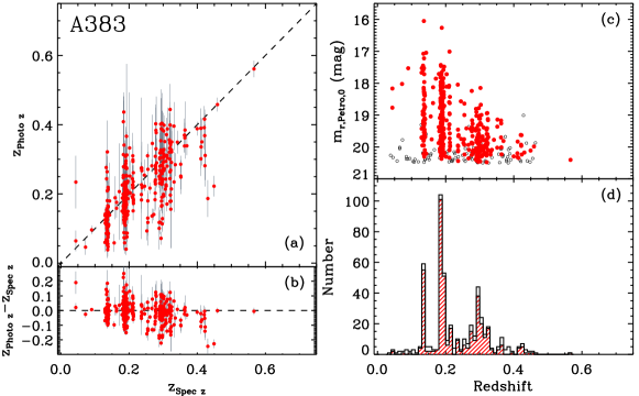
Figure 3.— (a-b) Comparison between photometric redshifts (Csabai et al., 2003) and spectroscopic redshifts for the galaxies with $m_{\rm r,Petro,0}<20.5$ inside the field of weak-lensing map (see Fig. 4). (c) $r$-band Petrosian magnitudes of galaxies with spectroscopic (red filled circles) and photometric (open circles) redshifts as a function of redshift. (d) Redshift distribution of galaxies with spectroscopic (red hatched histogram) and photometric (open histogram) redshifts.

To determine the membership of galaxies in each cluster, we use the caustic technique (Diaferio & Geller, 1997; Diaferio, 1999; Serra et al., 2011), originally devised to determine the mass profiles of galaxy clusters. The technique produces a useful tool for determining cluster membership. Analysis of galaxy clusters in a cosmological $N$-body simulation indicates that the caustic technique identifies true cluster members with $95$% completeness within 3$r_{200}$. The contamination of interlopers in the member galaxy catalog is only 2–8% at 1–3$r_{200}$ (Serra & Diaferio, 2013).

The caustic technique first uses the redshifts and the position on the sky of the galaxies to determine a hierarchical center of the cluster based on a binary tree analysis. We then plot the rest-frame clustercentric velocities of galaxies as a function of projected clustercentric radius centered on the hierarchical center. Figure 2 shows this phase-space diagram for each cluster; the expected trumpet-shaped pattern is obvious (Kaiser, 1987; Regos & Geller, 1989). The caustics (solid lines) generally agree with the lines based on a visual impression. They are cleanly defined especially at small radii. We use all the galaxies with measured redshifts regardless of their magnitudes for determining the membership, but restrict our analysis to the galaxies at $m_{\rm r,Petro,0}\leq 20.5$ within the weak-lensing maps for comparison between the galaxy number density and weak-lensing maps.

To segregate the red and blue cluster populations, we define a red sequence from a linear fit to the bright, red member galaxies in Figure 1 (e.g., $m_{\rm r,Petro,0}<19.5$ and $1<(g-r)_{\rm model,0}<2$ for A383). The solid line in each panel shows the red sequence for each cluster. The typical rms scatter ($\sigma$) around the red sequence is $\sim 0.1$ mag. A line $3\sigma$ blueward of the red sequence separates the red and blue members.

When we construct galaxy number density maps in Section 3.1, we also use SDSS photometric redshifts for galaxies without spectroscopic redshifts (Csabai et al., 2003). The rms uncertainties of photometric redshifts for the galaxies at $m_{r}<18$ and $m_{r}<21$ are $\sim$0.035 and $\sim$0.103, respectively (Csabai et al., 2003). The redshift range necessary for constructing galaxy number density maps to be compared with weak-lensing maps, is broad enough not to be significantly affected by these uncertainties.

As a prototypical example, we compare spectroscopic and photometric redshifts for galaxies in the field of A383 in the left panel of Figure 3. As expected, the photometric redshifts roughly agree with the spectroscopic redshifts with a large scatter. The top right panel shows $r$-band Petrosian magnitudes of galaxies with spectroscopic (red filled circles) and photometric (open circles) redshifts as a function of redshift. The bottom right panel shows the redshift histogram for each galaxy sample (red hatched and open histograms for spectroscopic and photometric redshifts, respectively). The foreground and background structures at $z\sim 0.14$ and $z\sim 0.3$, respectively ($z_{\rm A383}=0.1887$), are apparent in the histogram. As expected, the photometric redshifts contribute little; they are important mainly for faint galaxies. The comparison of spectroscopic and photometric redshifts for the other eight clusters is similar to A383, and we thus do not display them.

3. Results

Here we construct galaxy number density maps using several galaxy subsamples in Section 3.1, and cross correlate them with the weak-lensing maps in Section 3.2. We first test whether red cluster members can reproduce the main weak-lensing peak (see e.g., Zitrin et al. 2010), and then add other populations successively (i.e. foreground/background galaxies along the line of sight) to gauge their impact on the weak-lensing maps.

3.1. Galaxy Number Density Maps

To construct galaxy number density maps based on a spectroscopic sample of galaxies, it is important to understand any bias introduced by the spectroscopic observations, especially spectroscopic incompleteness. The pixel size and smoothing scale we need are set by the weak lensing maps of Okabe et al. (2010): e.g., 201$\times$201 pixels for the $20^{\prime}\times 20^{\prime}$ weak-lensing map and Gaussian smoothing scale of FWHM $=1\arcmin.2$ for A383.

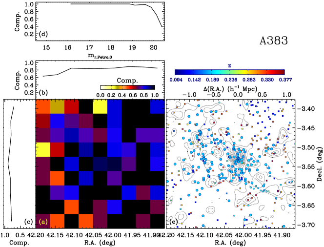
Figure 4.— (a) Two-dimensional spectroscopic completeness in the field of A383 as a function of right ascension and of declination. Integrated spectroscopic completeness as a function of right ascension (b), declination (c), and $r$-band magnitude (d). (e) Spatial distribution of galaxies at $m_{\rm r,Petro,0}\leq 20.5$ (open circles: members, squares: non-members inside the color bar redshift window, dots: non-members outside the color bar redshift window). Gray contours are the weak-lensing map of Okabe et al. (2010).

3.1.1 Spectroscopic Completeness

The left panel (a) of Figure 4 shows a two-dimensional map of the spectroscopic completeness for $m_{\rm r,Petro,0}\leq 20.5$ as a function of right ascension and declination, matched to the FOV of the weak-lensing map of A383. The two-dimensional completeness map is in 10$\times$10 pixels for the $20^{\prime}\times 20^{\prime}$ weak-lensing map. Panels (b-c) show the integrated completeness as a function of right ascension and declination, respectively. The overall completeness in this field is $\sim$81%. Although there are three pixels with a completeness $<50\%$, the completeness changes little with right ascension and declination. Panel (d) shows the integrated completeness as a function of $r$-band magnitude; it drops only at $m_{\rm r,Petro,0}>20$.

We also show the spatial distribution of galaxies superimposed on the A383 weak-lensing map of Okabe et al. (2010) in the right panel. Many member galaxies of A383 (open circles) are distributed around the peaks of the weak-lensing map, but some foreground and background galaxies (squares) are located around the peaks. The plots for other clusters are in the Appendix (see Figs. 14–17).

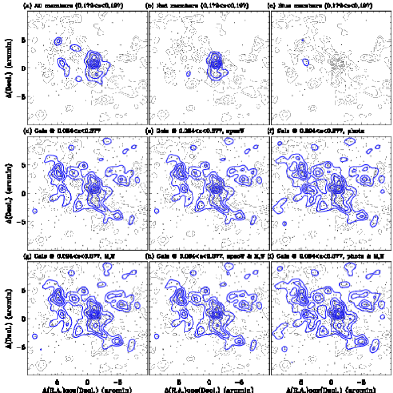
Figure 5.— A383 galaxy number density maps for several subsamples at $m_{\rm r,Petro,0}<20.5$. The lowest cluster surface number density contours is 1.61 galaxies arcmin^-2 and the contours increase in steps of 0.85 galaxy arcmin^-2. We smooth the contours with the Gaussian of FWHM $=1\arcmin.2$, the same smoothing scale as for weak-lensing maps of Okabe et al. (2010). Top row is for (a) all cluster members, (b) red cluster members, and (c) blue cluster members. Middle row is for the galaxies in the redshift range $0.5z_{\rm cl}\leq z\leq 2z_{\rm cl}$ (i.e., $0.094<z<0.377$ for A383): (d) without any weights, (e) weighted by spectroscopic completeness, and (f) complemented by galaxies with photometric redshifts. Bottom row is for the same sample as for in the middle row, but for weighted by stellar masses of galaxies as well: (g) without any weights, (h) weighted by spectroscopic completeness, and (i) complemented by galaxies with photometric redshifts.

3.1.2 Construction of Galaxy Number Density Maps: Revisiting A383

To study the relative contribution of cluster and foreground/background structure to the weak-lensing maps, we construct an extensive set of galaxy number density maps based on several galaxy subsamples. We smooth the contours with the same Gaussian FWHM as for the weak-lensing map of Okabe et al. (2010): e.g., FWHM$=1\arcmin.2$ for A383. We also use the same pixel size as for the weak lensing map (e.g., 201$\times$201 pixels for $20^{\prime}\times 20^{\prime}$ FOV of A383). Figure 5 shows these number density maps (blue contours) superimposed on the weak-lensing map (gray contours). The top panels are based on cluster member galaxies alone (all, red and blue members from left to right). We separate red and blue galaxies based on their positions in the $(g-r)_{\rm model,0}-m_{\rm r,Petro,0}$ color-magnitude diagram (see Section 2.2).

As in Geller et al. (2014a), the global morphology of the spatial distribution of cluster members alone (red and red plus blue populations) is similar to the shape of the main concentration in the weak-lensing map; both show a north-south elongation (see Panel a). The density map based on red members (Panel b) is also similar to the cluster shape in the weak-lensing map. Interestingly, blue members alone have little correspondence with the weak-lensing map (Panel c). This comparison supports the idea that the red population provides a reasonable tracer of the mass distribution of a galaxy cluster provided that the selection is dense and broad enough around the red sequence (Rines et al., 2013; Geller et al., 2014a). The comparison also suggests that the assumption that red cluster galaxies trace the dark matter distribution is a very reasonable approach for strong lensing models (Broadhurst et al., 2005; Zitrin et al., 2009; Medezinski et al., 2010).

The middle panels show contours for galaxies in the redshift range $0.5z_{\rm cl}\leq z\leq 2z_{\rm cl}$ (i.e., $0.094\leq z\leq 0.377$ for A383) where the contribution to the lensing signal may be significant (Hu, 1999). The number density map in Panel (d) is based on galaxies with measured redshifts. To account for galaxies without measured redshifts, we use two methods to construct the maps; we correct statistically for spectroscopic incompleteness and we use photometric redshifts. To correct for spectroscopic incompleteness, we compute the spectroscopic completeness for each object with a measured redshift in a three-dimensional parameter space: $r-$band magnitude, right ascension and declination. The right panels in Figure 4 show the spectroscopic completeness in this parameter space. We thus weight each galaxy by the inverse of the spectroscopic completeness to derive the galaxy number density map, and show it in Panel (e). We also use SDSS photometric redshifts for the galaxies without spectroscopic redshifts (see Section 2.2 for details). The corresponding number density map is in Panel (f).

In the bottom panels, we use the same galaxy samples as in middle panels, but additionally we weight each galaxy with the stellar mass. We compute stellar masses using the SDSS five-band photometric data with the Le Phare code (Arnouts et al., 1999; Ilbert et al., 2006). Details of the stellar mass estimates are in Zahid et al. (2014). Three panels show the maps based on galaxy samples of observed galaxies (g), weighted by spectroscopic completeness (h), and supplemented by photometric redshifts (i).

It is interesting that the global morphology of the number density maps in Panels (d–i) are similar despite the different correction methods. No matter how we weight the data, the correspondence between the galaxy number density and weak-lensing maps is more remarkable when we include foreground and background galaxies in the galaxy number density maps (Panels d–i), underscoring the contribution of large-scale structure along the line of sight to the weak-lensing signal.

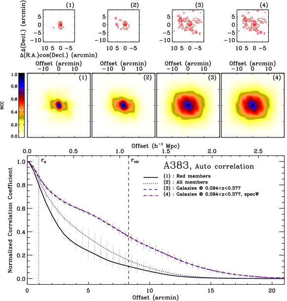
Figure 6.— Normalized auto correlation of A383 galaxy number density maps. (Top) Red contours indicate galaxy number density maps for four subsamples. (Middle) Two-dimensional normalized auto correlation maps. (Bottom) Azimuthally averaged correlation signal as a function of offset. Vertical dotted and dashed lines indicate $r_{s}$ and $r_{\rm vir}$ from Okabe et al. (2010), respectively.

3.2. Cross Correlation between Galaxy Number Density and Weak-lensing Maps

Here, we cross correlate the weak-lensing and galaxy number density maps for several of the galaxy subsamples. We use the normalized cross correlation (NCC), widely used in image processing (Gonzalez & Woods, 2002). It is defined by

$$NCC(x,y) = \frac{\sum\limits_{i,j}I_{1}(i,j)I_{2}(i+x,j+y)}{\sqrt{\sum\limits_{i,j}I_{1}^{2}(i,j)}\sqrt{\sum\limits_{i,j}I_{2}^{2}(i+x,j+y)}}$$ (1)

where $I_{1}(i,j)$ and $I_{2}(i,j)$ are pixel values of the galaxy number density and weak-lensing maps, respectively.

3.2.1 A383

To test our code and to understand what we can learn from the cross correlation, we first calculate the auto correlation for a galaxy number density map for a simulated cluster. We construct a mock galaxy catalog with 1000 galaxies in a cluster following the Navarro-Frenk-White profile (NFW; Navarro et al. 1997). We use the NFW profile of A383 with $r_{200}=1.184$ ($h^{-1}$Mpc) and $c_{200}=6.51$ derived in Newman et al. (2013), and we show the results in the Appendix (see Figs. 18 and 19). As expected, the normalized auto correlation signal is equal to unity at zero offset, and the correlation signal decreases with offset. It converges to zero at large radius (i.e. $r>r_{\rm 200}$); in other words, there is intrinsically no auto correlation signal at this radius and/or the auto correlation signal becomes small because at the edge of the maps.

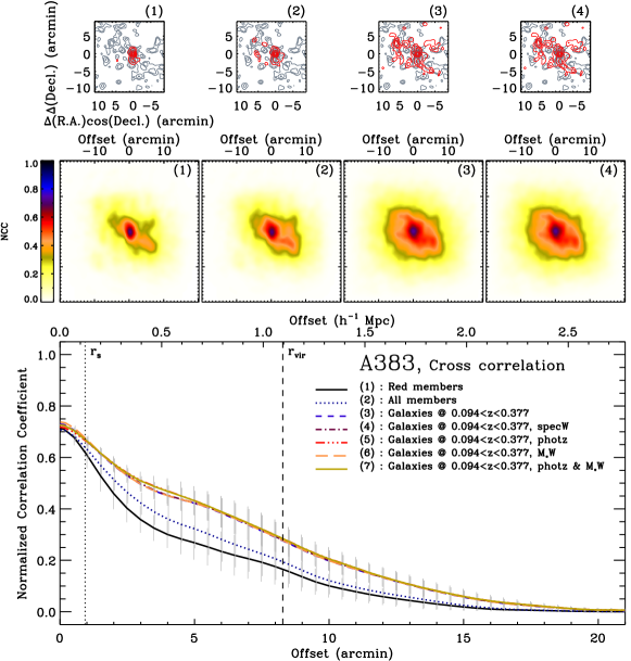
Figure 7.— Normalized cross correlation of A383 galaxy number density maps. (Top) Gray and red contours indicate weak-lensing and galaxy number density maps, respectively. We use seven galaxy subsamples listed in the bottom panel, but show only four examples. (Middle) Two-dimensional normalized cross correlation maps. (Bottom) Azimuthally averaged correlation signal as a function of offset. Vertical dotted and dashed lines indicate $r_{s}$ and $r_{\rm vir}$ from Okabe et al. (2010), respectively.

We also calculate the auto correlation for galaxy number density maps representing several galaxy subsamples of A383, and show the results in Figure 6. The top panels show the galaxy number density maps (red contours) for four subsamples: (1) red members, (2) all members, (3) galaxies at $0.5z_{\rm cl}\leq z\leq 2z_{\rm cl}$, and (4) galaxies at $0.5z_{\rm cl}\leq z\leq 2z_{\rm cl}$ weighted by their spectroscopic completeness (see Figure 4). The middle panels show the two-dimensional auto correlation map for each case. The bottom panel shows the azimuthally averaged auto correlation signal derived from each of the middle panel. The gray error bar indicates the dispersion in the two-dimensional correlation signal at each offset. As expected, the normalized correlation signal is unity at zero offset. The auto correlation signal converges to zero at $r>r_{\rm vir}$ for cases based on members alone (solid and dotted lines). However, the signal for cases including the galaxies at $0.5z_{\rm cl}\leq z\leq 2z_{\rm cl}$ (dashed and dot-dashed lines) is not negligible even at $r\sim r_{\rm vir}$, and decreases slowly; this effect results mainly from foreground and background galaxies along the line of sight that contribute to the auto correlation signal.

Figure 7 shows the results of cross correlating the galaxy number density maps and weak-lensing map. As in Figure 6, the top panels show the galaxy number density maps (red contours) for four galaxy subsamples superimposed on the weak-lensing maps (gray contours): (1) red members, (2) all members, (3) galaxies at $0.5z_{\rm cl}\leq z\leq 2z_{\rm cl}$, and (4) galaxies at $0.5z_{\rm cl}\leq z\leq 2z_{\rm cl}$ weighted by their spectroscopic completeness (see Figure 4). The middle panels show the two-dimensional cross correlation map for each case. We use seven galaxy subsamples in the cross correlation, but show only four cases in the top and middle panels for ease of view. The bottom panel shows the azimuthally averaged cross correlation signal for the seven galaxy subsamples.

Case (1) based on red member galaxies gives, not surprisingly, the narrowest correlation peak. The signal converges to zero at $r>r_{\rm vir}$ for the cases based on member galaxies alone (solid and dotted lines). The cases including galaxies at $0.5z_{\rm cl}\leq z\leq 2z_{\rm cl}$ (i.e., cases 3–7) are similar to one another, and show a broader distribution. The cross correlation signal is always larger than for the cases based on member galaxies alone, indicating the non-negligible contribution of foreground and background galaxies to the weak-lensing map.

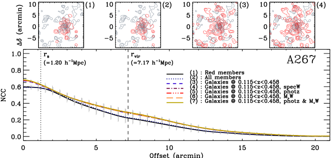
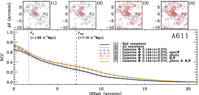
Figure 8.— Same as Fig. 7 (except for 2D NCC map), but for A267 and A611. Gray and red contours indicate weak-lensing and galaxy number density maps, respectively.

3.2.2 Comments on Individual Clusters

Here we discuss the cross correlation results for the other eight clusters. The plots for the eight clusters are in Figures 8–11 (see Fig. 7 for A383).

A267. The peak of the galaxy number density map based on members alone (top left panels) seems to be offset by $\sim$2^′ from the central peak of the lensing map, but the two peaks coincide when we include foreground and background galaxies in the number density map. The number density maps based on members alone show an overdensity only in the central region. When we include foreground and background galaxies in the map, several weak-lensing peaks other than the cluster appear in the number density map. Thus the normalized cross correlation signal including foreground and background galaxies exceeds those based on cluster members alone at zero offset. This excess can indicate a non-negligible contribution of foreground and background galaxies to the weak-lensing signal, but Okabe et al. (2010) found nothing unusual in deriving the weak-lensing mass profile for this cluster.

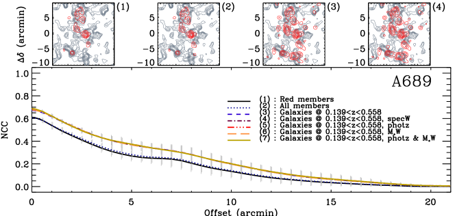
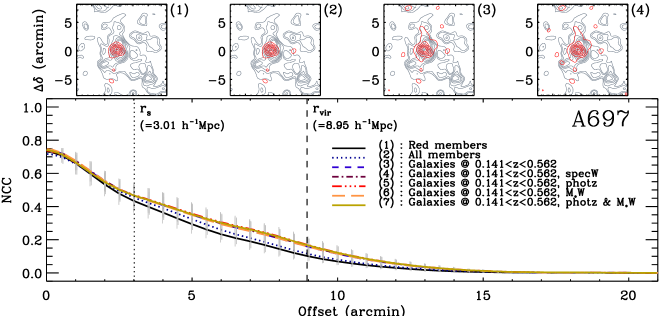
Figure 9.— Same as Fig. 7 (except for 2D NCC map), but for A689 and A697. Gray and red contours indicate weak-lensing and galaxy number density maps, respectively.

A611. This cluster is the most distant cluster ($z=0.288$) in the sample. The central region of the weak-lensing map shows a north/east-south/west elongation. The number density contours based on member galaxies alone weakly follow this elongation. However, the elongated contours are more similar to the weak-lensing contours when we include foreground and background galaxies. In other words, foreground and background galaxies can affect the apparent ellipticity of cluster mass distribution in a weak-lensing map. The mass profile of this cluster derived from the two-dimensional weak-lensing map is correspondingly very noisy (see Fig. 29 in Okabe et al. 2010). The noisy mass profile may result from the complex contribution of foreground and background galaxies to cluster shape.

A689. The X-ray emission of this cluster is dominated by a central BL Lac (Giles et al., 2012), thus an X-ray luminosity of this cluster is smaller than the other clusters in the sample (see Rines et al. 2013 for details). The weak-lensing map for this cluster shows several significant peaks. The galaxy number density maps based on members alone also show peaks in the central and upper regions of the map. The peaks in the lower regions of the map appear significantly enhanced when we include foreground and background galaxies. The cross correlation signal when we include foreground and background galaxies is systematically larger than the one based on members only. In fact, Okabe et al. (2010) could not derive the mass profile of this cluster because the projected mass distribution in the weak-lensing map is so complex. The difficulty in deriving the cluster mass profile occurs in part because the cluster itself is complex and the contribution of foreground and background galaxies further complicates the weak-lensing signal.

A697. The spectroscopic completeness for this cluster within the weak-lensing map is one of the highest (89%) in our sample. The cluster galaxies are centrally concentrated. They dominate the signal in the galaxy number density map even when we include foreground and background galaxies. Thus the radial profiles of the correlation signal for several subsamples do not differ significantly. Okabe et al. (2010) could not fit the mass profile of this cluster with an singular isothermal sphere (SIS) model, but could fit with either of cored isothermal sphere (CIS) or NFW models.

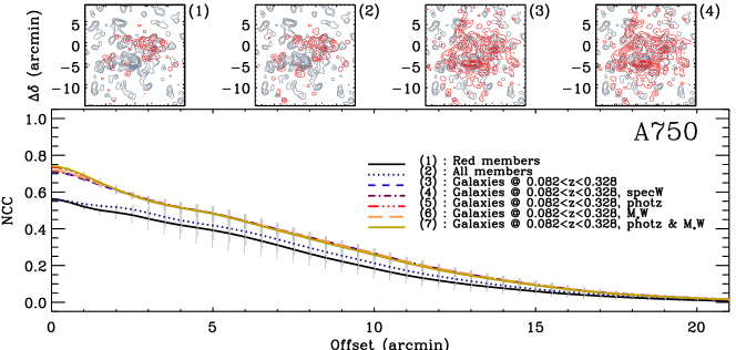
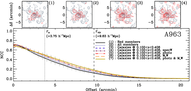
Figure 10.— Same as Fig. 7 (except for 2D NCC map), but for A750 and A963. Gray and red contours indicate weak-lensing and galaxy number density maps, respectively.

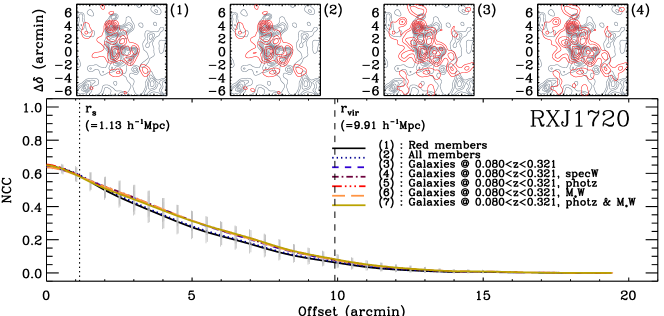
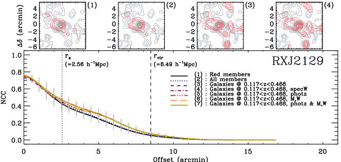
Figure 11.— Same as Fig. 7 (except for 2D NCC map), but for RXJ1720.1+2638 and RXJ2129.6+0005. Gray and red contours indicate weak-lensing and galaxy number density maps, respectively.

A750. This cluster is the closest cluster ($z=0.164$) in the sample. The difference in correlation signal at zero offset between cases based on members alone and including foreground/background galaxies is the largest in the sample. This result occurs because there are two clusters with similar redshifts aligned nearly along the line of sight in this field: $z=0.164$ for A750 and $z=0.1767$ for MS 0906.5+1110 (Carlberg et al., 1996; Rines et al., 2013; Geller et al., 2013). MS 0906.5+1110 is a more X-ray luminous than A750. Two clusters are often used without a clear distinction between the two. Their velocity difference is 3250 km s^-1 in the cluster rest frame. Our redshift survey resolves these two. The galaxies in MS 0906.5+1110 are not selected as A750 members, but contribute significantly to the lensing signal (see Section 5 of Geller et al. 2013 for details). Therefore, the mass based on weak lensing is roughly double the true cluster mass (Geller et al., 2013). In fact, Okabe et al. (2010) could not derive a mass profile of this cluster because the mass distribution in the weak-lensing map is so complex.

A963. At small offsets, the correlation signal when we include photometric redshifts for foreground and background galaxies are slightly smaller than the one based on members only. The large dispersion in the number density map based on foreground and background galaxies with photometric redshifts affects the normalization of the correlation signal (see eq 1). Considering the small difference and the large uncertainty in photometric redshifts, the effect is not statistically significant. Interestingly, Okabe et al. (2010) could not obtain an acceptable fit to the mass profile of this cluster with any of three models (NFW, SIS and CIS). This cluster is an exceptional case where weak lensing does not provide a robust mass profile even though the radial profiles of the cross correlation signal for several subsamples do not differ significantly.

RXJ1720.1+2638. The overall spectroscopic completeness for this cluster in the weak-lensing map is one of the highest (89%) in the sample. The Chandra X-ray observations show cold fronts in this cluster (Mazzotta et al., 2001), probably resulting from sloshing induced by the gravitational perturbation through minor mergers with small groups (Owers et al., 2011). A secondary peak to the north of the main concentration in the weak-lensing map appears as an overdensity in the number density map based on cluster members alone. The one-dimensional cross correlation signals are similar to one another, suggesting that the contribution of foreground and background galaxies to the weak-lensing map is not significant in this cluster field. Okabe et al. (2010) found a good fit to their models for a weak-lensing mass profile for this cluster.

RXJ2129.6+0005. This cluster has the smallest number of galaxies with spectroscopic redshifts in the weak-lensing map (N: 156). The secondary peaks to the west and to the south-southwest of the main concentration appear only when we include foreground and background galaxies, but the amplitudes of the peaks are low. Therefore, the one-dimensional correlation signal remains similar. Okabe et al. (2010) found a robust fit to the weak-lensing mass profile for this cluster.

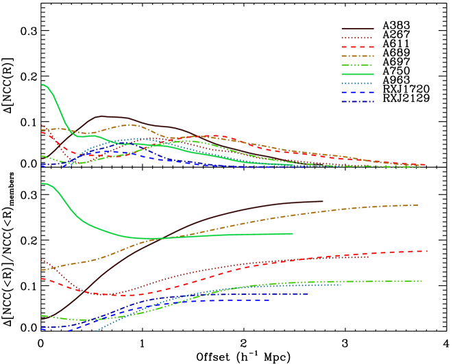
Figure 12.— (Top) Difference in normalized correlation signal for cases with cluster member galaxies (i.e., case 2 in Fig. 7) and with all the galaxies in the redshift range 0.5$z_{\rm cl}<z<2z_{\rm cl}$, complemented by photometric redshifts and weighed by stellar masses (i.e., case 7 in Fig. 7) as a function of offset for nine clusters in this study. (Bottom) Same as top panel, but for the cumulative fractional difference in normalized correlation signal.

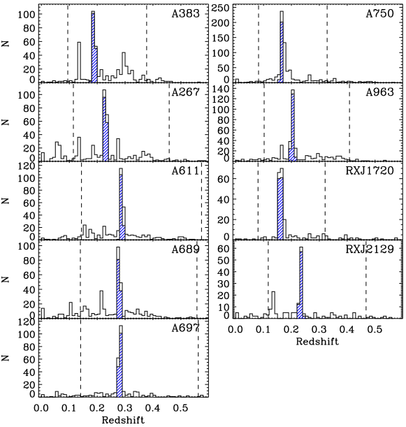
Figure 13.— Redshift histograms for the galaxies in the Subaru FOVs of galaxy clusters. Blue hatched histogram shows the cluster members. Open histograms show all the galaxies with spectroscopic or photometric redshifts at $m_{\rm r,Petro,0}<20.5$. Two vertical dashed lines indicate the redshift range when we include foreground and background galaxies (i.e., 0.5$z_{\rm cl}$ and 2$z_{\rm cl}$).

Comparison of the cross correlation results with the weak-lensing mass profiles in Okabe et al. (2010) for the nine clusters yields diverse results. There are three clusters (A689, A750 and A383) where the normalized cross correlation signal including foreground and background galaxies significantly exceeds the signal based on cluster members alone; Okabe et al. (2010) could not derive a stable mass profile for two clusters (e.g., A689 and A750) because of the complex projected mass distribution in the weak-lensing map, and could not obtain an acceptable fit to the mass profile of A383 with an NFW, SIS or CIS model. For two clusters where the normalized cross correlation signal including foreground and background galaxies slightly exceeds the signal based on cluster members alone at zero offset (e.g., A267, A611), Okabe et al. (2010) obtained a robust weak-lensing mass profile. Okabe et al. (2010) derived a stable weak-lensing mass profile for two clusters where there is no significant difference between the normalized cross correlation signal for several galaxy subsamples (e.g., RXJ1720.1+2638, RXJ2129.6+0005). Okabe et al. (2010) could not obtain an acceptable model fit to the derived mass profiles of two clusters (e.g., A697, A963) even though there is no significant difference in the normalized cross correlation signal for the galaxy subsamples we investigate here. Although the nine cluster show diverse results, a normalized cross correlation signal including foreground and background galaxies that significantly exceeds the signal based on cluster members alone appears to be a good proxy for an underlying systematic problem in the interpretation of the projected mass distribution as revealed by the weak-lensing map. Problems may result from resolved substructure within the cluster (e.g., A689) and/or from the contribution of large-scale structure superimposed along the line of sight (e.g., A383, A750).

4. DISCUSSION

We use dense redshift surveys in the fields of nine $z\sim 0.2$ galaxy clusters to cross correlate galaxy number density maps with weak-lensing maps. The cross correlation signal when we include foreground and background galaxies exceeds the one based on cluster members alone (see Figs 7–11); the cross correlation for the full sample is not negligible even outside the cluster virial radii.

We summarize the results of the cross correlation for the nine clusters in Figure 12. We plot the difference in the normalized correlation signal between the cases including all the galaxies around clusters and based on cluster members alone (i.e., case 7 and 2 in Fig. 7) in the top panel. The bottom panel shows the cumulative ($<$R), fractional excess for the case including all the galaxies around the cluster relative to the case based on cluster members alone (i.e., case 7 and 2 in Fig. 7).

The bottom panel shows that the cumulative fractional excess changes with offset, and increases up to 30%. The typical statistical error in the cumulative fractional excess is $3-5\%$. The nine clusters show different patterns, reflecting different large-scale structure along the line of sight. At the typical virial radius of our cluster samples (i.e., $\sim$ 1.3 $h^{-1}$Mpc), the cumulative fractional excess is 5–23%. These excesses are roughly consistent with the results based on simulation data (Hoekstra et al., 2011b); uncorrelated large-scale structure along the line of sight contributes to an uncertainty in weak-lensing cluster mass of $10-25\%$ for $z\sim 0.2$ clusters (see also Hoekstra 2001 for analytical prediction). The increase of the cumulative fractional excess with offset is also consistent with the idea that the weak-lensing analysis tends to overestimate cluster masses in the outer regions (e.g., see Fig. 13 in Geller et al. 2013). Studies of much larger cluster samples suggest that one can determine robust 3D mass profiles of galaxy clusters from weak lensing measurements based on the ensemble; a halo model approach to analysis of the ensemble can treat the correlated structure (Johnston et al., 2007a, b; Leauthaud et al., 2010).

One interesting aspect of Figure 12 is that the fractional excess is significant even at zero offset for some clusters (e.g., A267, A611, A689 and A750). Thus we might expect a significant number of galaxies inside the Subaru FOV that are not cluster members, but that contribute to the lensing signal. Figure 13 shows a redshift histogram for the galaxies in the weak-lensing map of each cluster. The hatched and open histograms show the cluster members and all the galaxies with spectroscopic/photometric redshifts at $m_{\rm r,Petro,0}\leq 20.5$, respectively. The histogram clearly shows that the fields of the clusters with large fractional excess have non-member galaxies close to the mean cluster redshift.

Based on simulations, Becker & Kravtsov (2011) emphasize that large-scale structure associated (or correlated) with individual clusters makes a non-negligible contribution ($\sim 20\%$) to the scatter of weak-lensing mass estimates in addition to the contribution of uncorrelated large-scale structure along the line of sight ($10-25\%$, Hoekstra et al. 2011b). We highlight the field of A750 in Section 3.2.2 where the contribution of the lensing signal from a nearby superimposed cluster is about a factor of two.

The vertical dashed lines in Figure 13 indicate the redshift range that we use to include foreground and background galaxies when we make the galaxy number density map for each cluster (i.e., 0.5$z_{\rm cl}$ and 2$z_{\rm cl}$). The nine clusters are at similar redshifts (i.e., $z\sim$0.2), thus the redshift ranges for including foreground and background galaxies are also similar. Moreover, examination of this plot also shows that the amplitude of the cumulative fractional excess in the bottom panel of Figure 12 does not depend on the cluster redshift, suggesting that the small difference in cluster redshifts in our sample does not introduce a bias.

The spectroscopic completeness of our redshift survey for the nine clusters is very high (70–89% at $m_{\rm r,Petro,0}\leq 20.5$). However, our redshift surveys are not deep enough to include a large number of galaxies at high redshift end of the lensing kernel (e.g., galaxies fainter than $m_{\rm r,Petro,0}=20.5$ at $0.1\lesssim z\lesssim 0.4$ for $z\sim 0.2$ cluster). Thus our estimates of the contribution of large-scale structure along the line of sight to the cluster lensing maps could be lower limits; the real contribution could be larger even though photometric redshifts mitigate this issue to some extent.

Okabe et al. (2010) studied the mass profiles of the nine clusters in this study derived from the two-dimensional weak-lensing maps. They used three mass models to fit the derived mass profiles: NFW, SIS and CIS. Interestingly, they could not derive the mass profiles of A750 and A689 because the mass distribution in the weak-lensing maps is complex in these systems. They could fit the mass profiles with their three models for most clusters, but could not obtain an acceptable fit to the mass profile of A383 with any model. These three clusters (A383, A689 and A750) show the largest fractional excesses ($11-30\%$) in the integrated normalized correlation signal at offset $>$0.5 $h^{-1}$ Mpc. The range of possible impacts of the superimposed structure on cluster mass estimates is large: a few percent for A383 (Geller et al., 2014a), and up to a factor of two for A750 (Geller et al., 2013). These results suggest that the excess in the integrated cross correlation signal could be a useful proxy for assessing the reliability of weak-lensing cluster mass estimates.

We cross correlate two independent measurements, the galaxy number density map and the lensing convergence field, $\kappa$ for each cluster. As suggested by Van Waerbeke et al. (2013), it would be interesting to use the galaxy number density map to reconstruct a model convergence map for comparison with the observed one. However, this procedure requires knowledge positions and redshifts of the source galaxies that are not currently available.

5. CONCLUSIONS

We use dense redshift surveys in the fields of nine $z\sim 0.2$ galaxy clusters to compare the structures identified in weak-lensing and galaxy number density maps. We combine 2087 new MMT/Hectospec redshifts and the data in the literature to make the overall spectroscopic completeness in the weak-lensing maps high (70–89%) and uniform. With these dense redshift surveys, we first construct galaxy number density maps using several galaxy subsamples. Our primary results are:

1. The global morphology of the spatial distribution of cluster members alone is similar to the shape of the cluster peak in weak-lensing maps. However, in some clusters (e.g., A611), the apparent shape of the cluster peak in the weak-lensing map may be affected by the contribution of foreground and background galaxies.

2. The red cluster galaxies dominate the cluster weak-lensing signal, and blue cluster galaxies contribute little to the number density maps of cluster members. These results suggest that the red populations are reliable tracers of the mass distribution of galaxy clusters provided that the selection is dense and broad enough around the red sequence. This result supports the approach often taken in strong lensing analysis (Broadhurst et al., 2005; Zitrin et al., 2009; Medezinski et al., 2010).

3. The correspondence between the galaxy number density and weak-lensing maps is even more remarkable when we include foreground and background galaxies in the galaxy number density maps, reflecting the contribution of superimposed large-scale structure along the line of sight to the $\kappa$ map.

We cross correlate the galaxy number density maps with the weak-lensing maps, and we find:

1. The cross correlation signal when we include foreground and background galaxies at 0.5$z_{\rm cl}<z<2z_{\rm cl}$ is always larger than for the case with cluster members alone. The fractional excess of the integrated normalized correlation signal for the case including foreground and background galaxies relative to the case base on cluster members alone is $10-23$% at the cluster virial radius. This excess can be as high as 30% depending on the cluster.

2. Superimposed structure close to the cluster in redshift space contributes to the weak-lensing peaks more significantly than unrelated large-scale structure along the line of sight.

3. The mass profiles of three clusters (A383, A689 and A750) with the largest fractional excesses ($11-30\%$) of the integrated normalized correlation signal are also not well constrained in weak lensing (Okabe et al., 2010). Thus the excess in the integrated normalized correlation signal could be a useful proxy for assessing the reliability of weak-lensing cluster mass estimates.

A dense redshift survey of galaxy clusters is important for understanding the meaning of a weak-lensing $\kappa$ map. We plan to extend this study to a larger cluster sample including merging clusters in a forthcoming paper (H. S. Hwang et al., in preparation).

Future exploration with deep spectroscopic or even photometric redshift surveys covering all the galaxies including faint ones in the lensing kernel is important for refining the estimates of the contribution of large-scale structure along the line of sight accurately. To resolve the structure near clusters that contribute to weak-lensing maps significantly, a spectroscopic survey is crucial. Techniques that treat the redshift survey simultaneously with weak lensing may eventually provide very powerful probes of mass distribution uncontaminated by superimposed structure along the line of sight.

Facility: MMT

Appendix A Appendix Material

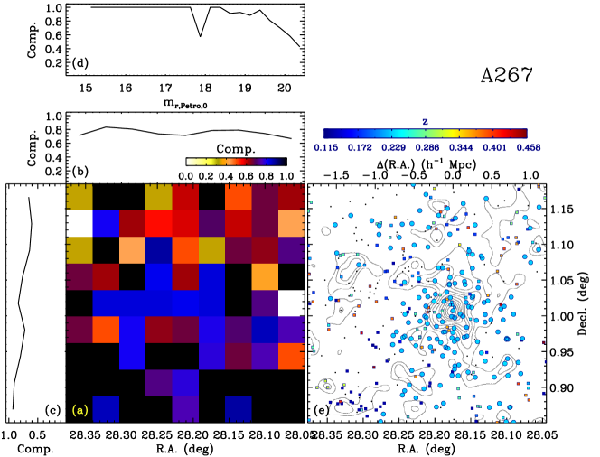
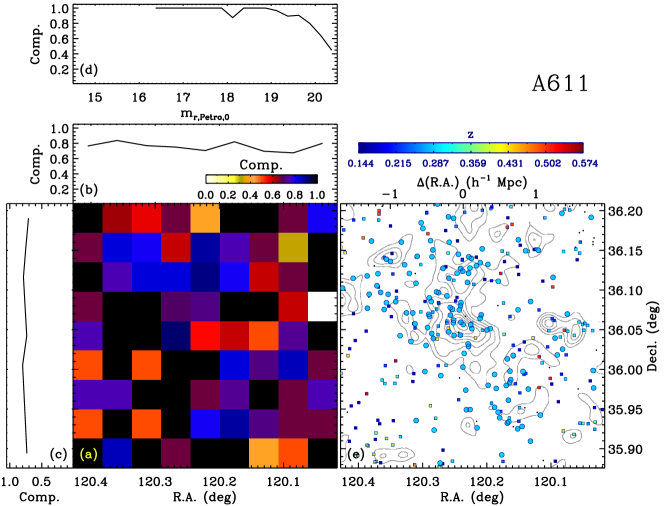
Figure 14.— Same as Fig. 4, but for A267 and A611.

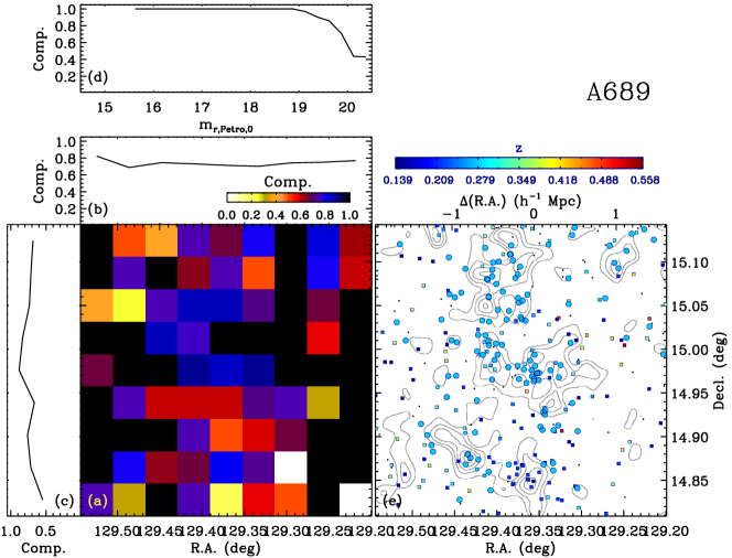
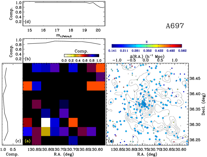
Figure 15.— Same as Fig. 4, but for A689 and A697.

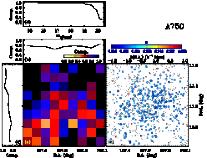
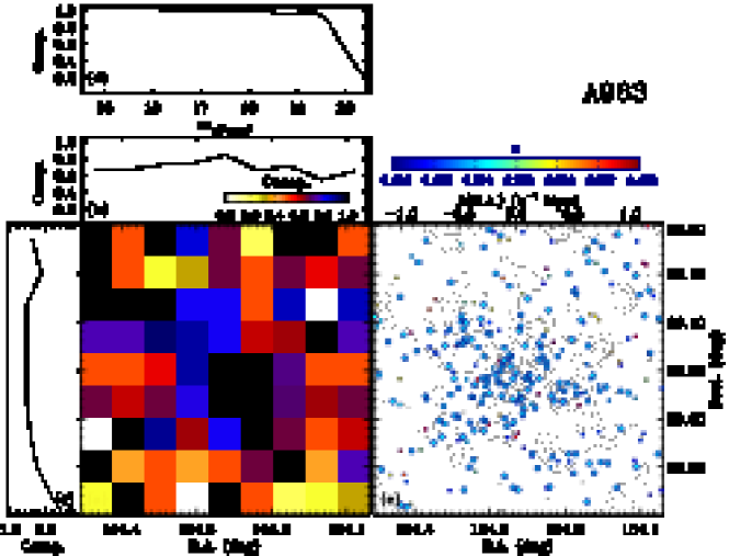
Figure 16.— Same as Fig. 4, but for A750 and A963.

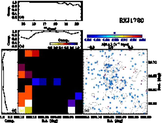
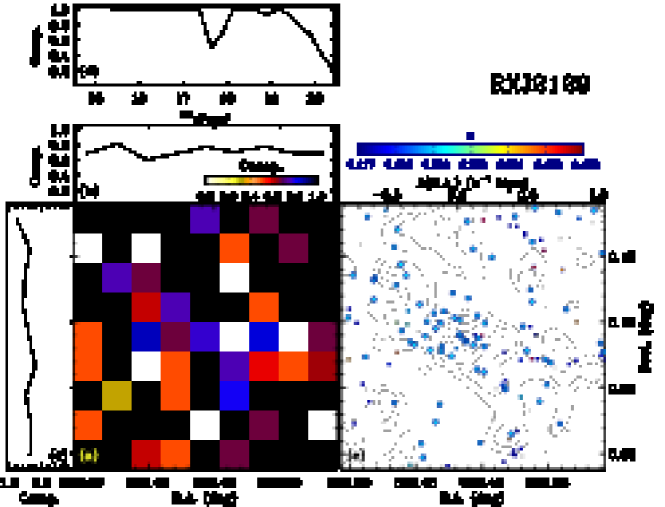
Figure 17.— Same as Fig. 4, but for RXJ1720.1+2638 and RXJ2129.6+0005.

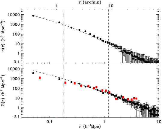
Figure 18.— (Top) Galaxy number density profile for a simulated cluster (filled circles). Dashed line is the input NFW profile with $r_{200}=1.184$ ($h^{-1}$Mpc) and $c_{200}=6.51$ (Newman et al., 2013). Vertical dotted and dashed lines indicate $r_{s}$ and $r_{200}$, respectively. (Bottom) Same as top panel, but for projected galaxy number density profile. Red squares are observed galaxy number density profile of A383 after completeness correction derived in this study.

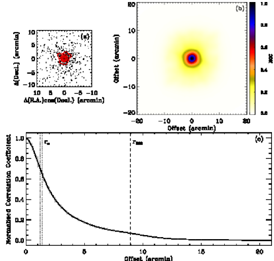
Figure 19.— Normalized auto correlation of the galaxy number density map for a simulated cluster. (Top left) Spatial distribution of galaxies (black dots) with galaxy number density contours (red). (Top right) Two-dimensional normalized auto correlation map. (Bottom) Azimuthally averaged correlation signal as a function of offset. Vertical dot-dashed, dotted and dashed lines indicate a smoothing scale FWHM$=1^{\prime}.2$, $r_{s}$ and $r_{200}$, respectively.

References

- Ahn et al. (2014) Ahn, C. P., Alexandroff, R., Allende Prieto, C., et al. 2014, ApJS, 211, 17
- Arnouts et al. (1999) Arnouts, S., Cristiani, S., Moscardini, L., et al. 1999, MNRAS, 310, 540
- Bahé et al. (2012) Bahé, Y. M., McCarthy, I. G., & King, L. J. 2012, MNRAS, 421, 1073
- Becker & Kravtsov (2011) Becker, M. R., & Kravtsov, A. V. 2011, ApJ, 740, 25
- Broadhurst et al. (2005) Broadhurst, T., Benítez, N., Coe, D., et al. 2005, ApJ, 621, 53
- Carlberg et al. (1996) Carlberg, R. G., Yee, H. K. C., Ellingson, E., et al. 1996, ApJ, 462, 32
- Clowe et al. (2006) Clowe, D., Bradač, M., Gonzalez, A. H., et al. 2006, ApJ, 648, L109
- Coe et al. (2012) Coe, D., Umetsu, K., Zitrin, A., et al. 2012, ApJ, 757, 22
- Coupon et al. (2013) Coupon, J., Broadhurst, T., & Umetsu, K. 2013, ApJ, 772, 65
- Csabai et al. (2003) Csabai, I., Budavári, T., Connolly, A. J., et al. 2003, AJ, 125, 580
- Diaferio (1999) Diaferio, A. 1999, MNRAS, 309, 610
- Diaferio & Geller (1997) Diaferio, A., & Geller, M. J. 1997, ApJ, 481, 633
- Dodelson (2004) Dodelson, S. 2004, Phys. Rev. D, 70, 023008
- Drinkwater et al. (2010) Drinkwater, M. J., Jurek, R. J., Blake, C., et al. 2010, MNRAS, 401, 1429
- Duffy et al. (2008) Duffy, A. R., Schaye, J., Kay, S. T., & Dalla Vecchia, C. 2008, MNRAS, 390, L64
- Fabricant et al. (2005) Fabricant, D., Fata, R., Roll, J., et al. 2005, PASP, 117, 1411
- Geller et al. (2005) Geller, M. J., Dell’Antonio, I. P., Kurtz, M. J., et al. 2005, ApJ, 635, L125
- Geller et al. (2013) Geller, M. J., Diaferio, A., Rines, K. J., & Serra, A. L. 2013, ApJ, 764, 58
- Geller et al. (2014a) Geller, M. J., Hwang, H. S., Diaferio, A., et al. 2014a, ApJ, 783, 52
- Geller et al. (2014b) Geller, M. J., Hwang, H. S., Fabricant, D. G., et al. 2014b, ApJS, 213, 35
- Geller et al. (2010) Geller, M. J., Kurtz, M. J., Dell’Antonio, I. P., Ramella, M., & Fabricant, D. G. 2010, ApJ, 709, 832
- Giles et al. (2012) Giles, P. A., Maughan, B. J., Birkinshaw, M., Worrall, D. M., & Lancaster, K. 2012, MNRAS, 419, 503
- Girardi et al. (2006) Girardi, M., Boschin, W., & Barrena, R. 2006, A&A, 455, 45
- Gonzalez & Woods (2002) Gonzalez, R. C., & Woods, R. E. 2002, Digital image processing (2nd ed.; Upper Saddle River, NJ: Prentice-Hall)
- Gruen et al. (2011) Gruen, D., Bernstein, G. M., Lam, T. Y., & Seitz, S. 2011, MNRAS, 416, 1392
- Hoekstra (2001) Hoekstra, H. 2001, A&A, 370, 743
- Hoekstra (2003) —. 2003, MNRAS, 339, 1155
- Hoekstra (2007) —. 2007, MNRAS, 379, 317
- Hoekstra et al. (2011a) Hoekstra, H., Donahue, M., Conselice, C. J., McNamara, B. R., & Voit, G. M. 2011a, ApJ, 726, 48
- Hoekstra et al. (2011b) Hoekstra, H., Hartlap, J., Hilbert, S., & van Uitert, E. 2011b, MNRAS, 412, 2095
- Hu (1999) Hu, W. 1999, ApJ, 522, L21
- Huterer (2010) Huterer, D. 2010, General Relativity and Gravitation, 42, 2177
- Huterer et al. (2013) Huterer, D., Kirkby, D., Bean, R., et al. 2013, arXiv (1309.5385)
- Ilbert et al. (2006) Ilbert, O., Arnouts, S., McCracken, H. J., et al. 2006, A&A, 457, 841
- Jaffé et al. (2013) Jaffé, Y. L., Poggianti, B. M., Verheijen, M. A. W., Deshev, B. Z., & van Gorkom, J. H. 2013, MNRAS, 431, 2111
- Johnston et al. (2007a) Johnston, D. E., Sheldon, E. S., Tasitsiomi, A., et al. 2007a, ApJ, 656, 27
- Johnston et al. (2007b) Johnston, D. E., Sheldon, E. S., Wechsler, R. H., et al. 2007b, ArXiv (0709.1159)
- Kaiser (1987) Kaiser, N. 1987, MNRAS, 227, 1
- Kurtz et al. (2012) Kurtz, M. J., Geller, M. J., Utsumi, Y., et al. 2012, ApJ, 750, 168
- Leauthaud et al. (2010) Leauthaud, A., Finoguenov, A., Kneib, J.-P., et al. 2010, ApJ, 709, 97
- Lemze et al. (2013) Lemze, D., Postman, M., Genel, S., et al. 2013, ApJ, 776, 91
- Mazzotta et al. (2001) Mazzotta, P., Markevitch, M., Vikhlinin, A., et al. 2001, ApJ, 555, 205
- Medezinski et al. (2010) Medezinski, E., Broadhurst, T., Umetsu, K., et al. 2010, MNRAS, 405, 257
- Miyazaki et al. (2002) Miyazaki, S., Komiyama, Y., Sekiguchi, M., et al. 2002, PASJ, 54, 833
- Navarro et al. (1997) Navarro, J. F., Frenk, C. S., & White, S. D. M. 1997, ApJ, 490, 493
- Newman et al. (2013) Newman, A. B., Treu, T., Ellis, R. S., et al. 2013, ApJ, 765, 24
- Okabe et al. (2010) Okabe, N., Takada, M., Umetsu, K., Futamase, T., & Smith, G. P. 2010, PASJ, 62, 811
- Okabe & Umetsu (2008) Okabe, N., & Umetsu, K. 2008, PASJ, 60, 345
- Owers et al. (2011) Owers, M. S., Nulsen, P. E. J., & Couch, W. J. 2011, ApJ, 741, 122
- Prada et al. (2012) Prada, F., Klypin, A. A., Cuesta, A. J., Betancort-Rijo, J. E., & Primack, J. 2012, MNRAS, 423, 3018
- Regos & Geller (1989) Regos, E., & Geller, M. J. 1989, AJ, 98, 755
- Rines et al. (2013) Rines, K., Geller, M. J., Diaferio, A., & Kurtz, M. J. 2013, ApJ, 767, 15
- Serra & Diaferio (2013) Serra, A. L., & Diaferio, A. 2013, ApJ, 768, 116
- Serra et al. (2011) Serra, A. L., Diaferio, A., Murante, G., & Borgani, S. 2011, MNRAS, 412, 800
- Shan et al. (2012) Shan, H., Kneib, J.-P., Tao, C., et al. 2012, ApJ, 748, 56
- Starikova et al. (2014) Starikova, S., Jones, C., Forman, W. R., et al. 2014, ApJ, 786, 125
- Umetsu et al. (2014) Umetsu, K., Medezinski, E., Nonino, M., et al. 2014, ApJ, in press (arXiv:1404.1375)
- Utsumi et al. (2014) Utsumi, Y., Miyazaki, S., Geller, M. J., et al. 2014, ApJ, 786, 93
- Van Waerbeke et al. (2013) Van Waerbeke, L., Benjamin, J., Erben, T., et al. 2013, MNRAS, 433, 3373
- Zahid et al. (2014) Zahid, J., Dima, G., Kudritzki, R., et al. 2014, ApJ, 791, 130
- Zitrin et al. (2009) Zitrin, A., Broadhurst, T., Umetsu, K., et al. 2009, MNRAS, 396, 1985
- Zitrin et al. (2010) —. 2010, MNRAS, 408, 1916