Counting rational points on the
Cayley ruled cubic

Abstract.

We count rational points of bounded height on the Cayley ruled cubic surface and interpret the result in the context of general conjectures due to Batyrev and Tschinkel.

1. Introduction

The arithmetic of singular cubic surfaces $S\subset\mathbb{P}^{3}$ has long been the subject of intensive study. When $S$ is defined over $\mathbb{Q}$ and has isolated ordinary singularities then the set $S(\mathbb{Q})$ of rational points on $S$ is Zariski dense in $S$ as soon as it is non-empty. Under this hypothesis, a finer measure of density is achieved by studying the counting function

$$N(U;B)=\#\{t\in U(\mathbb{Q}):H(t)\leqslant B\},$$

where $H:S(\mathbb{Q})\to\mathbb{R}_{>0}$ is an anticanonical height function and $U\subset S$ is obtained by deleting the lines from $S$.

The conjectures of Manin [FMT89] and Peyre [Pey03] give a precise prediction for the asymptotic behaviour of $N(U;B)$, as $B\rightarrow\infty$, for normal del Pezzo surfaces in terms of certain invariants associated to a minimal resolution. The conjecture has now been resolved for several singular cubic surfaces over $\mathbb{Q}$. Most recently, for example, Le Boudec [LeB14] has handled a cubic surface with singularity type $\mathbf{D}_{4}$ (see the references therein for earlier work on this topic). However, the conjectures of Manin and Peyre offer no prediction for cubic surfaces with non-isolated singularities. Indeed, the asymptotics for such surfaces are different as they contain infinitely many lines.

The primary goal of this paper is to study the counting function for a particular non-normal cubic surface and to show that the resulting asymptotic formula can still be interpreted in the context of a much more general suite of conjectures due to Batyrev and Tschinkel [BT98b]. According to Dolgachev [Dol12, Thm 9.2.1], any irreducible non-normal cubic surface over $\mathbb{Q}$ is either a cone over an irreducible singular plane cubic, or it is projectively equivalent to one of the (non-isomorphic) surfaces

$$t_{0}^{2}t_{2}-t_{1}^{2}t_{3}=0$$ (1.1)

or

$$t_{0}t_{1}t_{2}-t_{0}^{2}t_{3}-t_{1}^{3}=0,$$ (1.2)

both of which are singular along the line $t_{0}=t_{1}=0$. These surfaces arise as different projections of the cubic scroll in $\mathbb{P}^{4}$, which is isomorphic to the (ruled) Hirzebruch surface $\mathbb{F}_{1}$ (i.e. a del Pezzo surface of degree $8$).

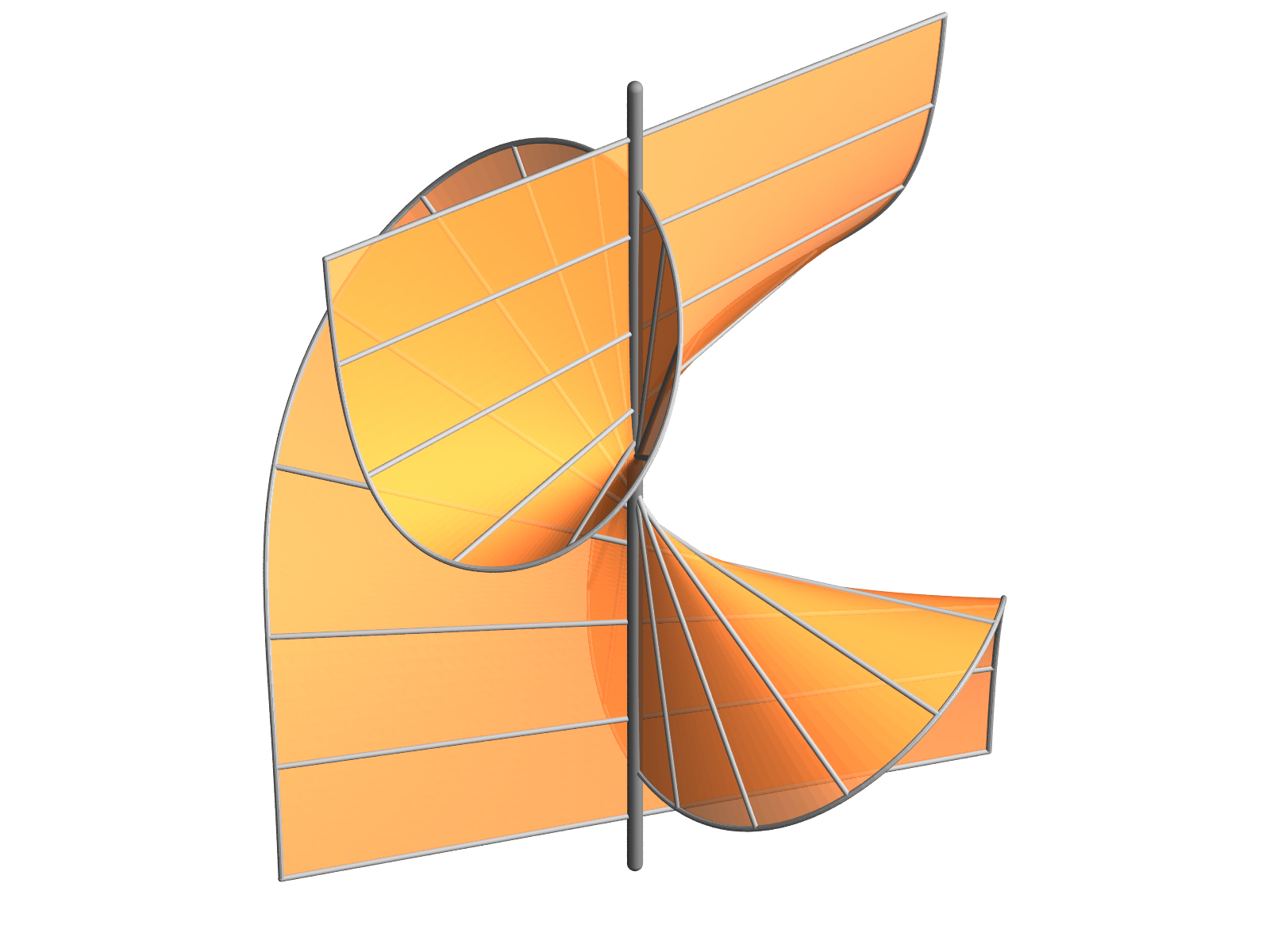
Figure 1. The Cayley ruled cubic surface

For the remainder of this paper we will focus exclusively on the cubic surface (1.2), illustrated in Figure 1. This is called the Cayley ruled surface and we will denote it by $W\subset\mathbb{P}^{3}$. While (1.1) is plainly toric the Cayley surface is not toric. Indeed, according to Gmeiner and Havlicek [GH13, Lemma 3.1], the automorphism group of $W$ is a 3-dimensional algebraic group, which contains a 2-dimensional unipotent subgroup. Thus there is no $2$-dimensional torus acting faithfully on $W$.

Let $V=W\setminus\{t_{0}=t_{1}=0\}$ be the complement of the double line in $W$. Clearly $V\cong\mathbb{A}^{2}$. Finally, we take our height function $H:V(\mathbb{Q})\to\mathbb{R}_{>0}$ to be metrized by the Euclidean norm. (i.e. $H(t)=\|\mathbf{t}\|:=\sqrt{t_{0}^{2}+\dots+t_{3}^{2}}$ if $t$ is represented by a primitive vector $\mathbf{t}\in\mathbb{Z}_{\mathrm{prim}}^{4}$.) It then follows from a computation of Serre [Ser97, §2.12] that $N(V;B)=O_{V}(B^{2})$. We are able to establish a precise asymptotic formula, as follows.

Theorem 1.1.

We have

$$N(V;B)=\frac{\pi B^{2}}{2\zeta(2)}\sum_{\begin{subarray}{c}(\lambda,\mu)\in\mathbb{Z}_{\mathrm{prim}}^{2}\\ \mu\neq 0\end{subarray}}\frac{1}{\sqrt{f(\lambda,\mu)}}+O(B^{3/2}\log B),$$

where $f(\lambda,\mu)=\lambda^{6}+2\lambda^{4}\mu^{2}+\lambda^{2}\mu^{4}+\mu^{6}$.

Since $W$ is not toric this result is not implied by work of Batyrev and Tschinkel [BT98a]. In §2 we will prove that this result is compatible with some very general conjectures of Batyrev and Tschinkel [BT98b] about “weakly $\mathscr{L}$-saturated” smooth quasi-projective varieties. The first step involves constructing an explicit desingularisation of $W$, which we record here for the sake of convenience.

Theorem 1.2.

Let $X\subset\mathbb{P}^{2}\times\mathbb{P}^{1}$ be the biprojective surface with coordinates $(x_{0},x_{1},x_{2};y_{1},y_{2})$ defined by $x_{1}y_{2}=x_{2}y_{1}$. Then the morphism $\varphi:X\to W$ defined by

$$\varphi(x_{0},x_{1},x_{2};y_{1},y_{2})=(x_{1}y_{1},x_{1}y_{2},x_{0}y_{1}+x_{2}y_{2},x_{0}y_{2})$$

is a desingularisation of $W$ such that the open subvariety $U$ of $X$ where $x_{1}\neq 0$ is sent isomorphically onto the subset $V$ of W where $t_{0}\neq 0$.

The surface $X$ is isomorphic to $\mathbb{F}_{1}$ and it is also the normalisation of $W$ (see Remark 2.1). Despite starting with an anticanonical counting problem for the singular cubic surface $W$, Theorem 1.2 leads to a counting problem for the non-singular surface $X$, endowed with an ample but non-anticanonical linear system. For $m>1$, Billard [Bil98] has provided precise asymptotics for counting functions associated to the Hirzebruch surface $\mathbb{F}_{m}$ endowed with a general complete linear system. For $m=1$, the case of primary interest to us, work of Chambert-Loir and Tschinkel [CLT00, Thm. 4.16] handles the corresponding counting problem associated to a particular choice of metric.

We will offer two very different proofs of Theorem 1.1. It should be emphasised that both methods are capable of producing asymptotic formulae for counting functions associated to other non-normal surfaces. Handling the cubic surface (1.1), for example, is easier than $W$ and leads to similar asymptotic behaviour.

The simplest proof of Theorem 1.1 is found in §3. It relies on an explicit realisation of the Fano variety $F_{1}(W)\subset\mathbb{G}(1,3)\subset\mathbb{P}^{5}$, parametrising lines on $W$, as the union of an isolated point and a twisted cubic. A standard result from the geometry of numbers is then invoked to handle the contribution from the rational points on the lines.

The second approach is found in §4. It uses the fact that $W$ is an equivariant compactification of the additive algebraic group $\mathbb{G}_{a}^{2}$, in order to study the analyticity of the associated height zeta function using adelic Poisson summation. This argument is modelled on the methods of Chambert-Loir and Tschinkel [CLT00, §3], which were developed to study equivariant compactifications of vector groups. A noteworthy feature of the proof is that we get contributions to the main term from some of the non-trivial characters. The counting function $N(V;B)$ can be interpreted as a counting function on $X$ endowed with an ample line bundle of bidegree $(1,1)$ and a certain metric which is inherited from the singular model $W$ (see §2). This counting function is related to the counting function on $X$ considered in [CLT00, Thm. 4.16], but the latter does not imply Theorem 1.1 since it involves a different metric.

Remark 1.3.

Although we are concerned here with rational points on $W$, the problem of counting integer points on any affine model is also of interest. For either of the affine surfaces $xyz=x^{2}+y^{3}$ or $xy=x^{2}z+y^{3}$ it is possible to show that the number of integers $(x,y,z)\in(\mathbb{Z}\cap[-B,B])^{3}$ has order of magnitude $B$. This is in agreement with the affine surface hypothesis proposed in [BHBS06].

Acknowledgements.

While working on this paper the first author was supported by an IUF Junior and the second author was supported by ERC grant 306457. The authors are very grateful to Professor Hans Havlicek for allowing us to include Figure 1 which was created by him, and to the anonymous referee for some useful comments.

2. The Batyrev–Tschinkel conjecture

Let us begin by establishing Theorem 1.2. Let $\pi:X\to\mathbb{P}^{2}$ be the projection from $(x_{0},x_{1},x_{2};y_{1},y_{2})$ to $(x_{0},x_{1},x_{2})$ and let $O_{1}\subset\mathbb{P}^{2}$ be the open subset where $x_{1}\neq 0$. Then $\pi$ restricts to an isomorphism $\pi_{1}:U\to O_{1}$. Next, let $O\subset\mathbb{P}^{2}$ be the open subset where $(x_{1},x_{2})\neq(0,0)$. There is then a morphism $f:O\to V$ defined by $t_{i}=Q_{i}(x_{0},x_{1},x_{2})$, for $0\leqslant i\leqslant 3$, where

$$Q_{0}(x_{0},x_{1},x_{2}) =x_{1}^{2},$$

$$Q_{1}(x_{0},x_{1},x_{2}) =x_{1}x_{2},$$

$$Q_{2}(x_{0},x_{1},x_{2}) =x_{0}x_{1}+x_{2}^{2},$$

$$Q_{3}(x_{0},x_{1},x_{2}) =x_{0}x_{2}.$$

This morphism restricts to an isomorphism $f_{1}:O_{1}\to V$, with corresponding inverse $V\to O_{1}$ such that $(1,t_{1}/t_{0},t_{2}/t_{0},t_{3}/t_{0})$ is sent to

$$(x_{0}/x_{1},1,x_{2}/x_{1})=(-(t_{1}/t_{0})^{2}+t_{2}/t_{0},1,t_{1}/t_{0}).$$

Since $\varphi=f_{1}\circ\pi_{1}$ on $U$, it follows that $\varphi$ restricts to an isomorphism $\varphi:U\to V$, as desired.

Remark 2.1.

The morphism $\varphi:X\to W$ is finite since it is projective and quasi-finite (see [Har77, Ex. III.11.2]). Since $\varphi$ is birational, furthermore, it is therefore the normalisation of $W$ (see [GW10, Ex. 12.20]).

We now proceed to recast the counting function $N(V;B)$ in the language of adelic metrics. Let $|\cdot|_{p}$ be the usual absolute value on $\mathbb{Q}_{p}$ defined by $|p^{\nu}x|_{p}=p^{-\nu}$ if $\nu\in\mathbb{Z}$ and $x\in U_{p}=\mathbb{Z}_{p}^{*}$. Let $M=\mathscr{O}_{W}(1)$ and let $s_{0},\dots,s_{3}$ be the global sections of $M$ given by the coordinates $t_{0},\dots,t_{3}$ of $\mathbb{P}^{3}$. We may then define a $p$-adic norm $\|\cdot\|_{p}$ on $M$ by

$$\|s(w_{p})\|_{p}=\min_{i}|(s/s_{i})(w_{p})|_{p},$$

for a local section $s$ of $M$ at a point $w_{p}\in W(\mathbb{Q}_{p})$ and where $i\in\{0,1,2,3\}$ runs over the global sections $s_{i}$ such that $s_{i}(w_{p})\neq 0$. At the archimedean place we define a real norm $\|\cdot\|_{\infty}$ on $M$ by

$$\|s(w_{\infty})\|_{\infty}=\left(\sum_{i}|s_{i}/s(w_{\infty})|^{2}\right)^{-1/2}$$ (2.1)

for a local section $s\neq 0$ of $M$ at a point $w_{\infty}\in W(\mathbb{R})$.

Now let $\|\cdot\|_{v}$ denote $\|\cdot\|_{\infty}$ or $\|\cdot\|_{p}$ for a prime $p$. Then we get an adelic metric $(\|\cdot\|_{v})$ on $M$ as in Peyre [Pey95] and a height on $W(\mathbb{Q})$ defined by

$$H(w)=\prod_{v}\|s(w)\|_{v}^{-1},$$

for a rational point $w$ on $W$ and a local section $s$ of $M$ with $s(w)\neq 0$. This height does not depend on the choice of $s$. For a rational point $P$ on $V$ represented by $(1,t_{1},t_{2},t_{3})$, we may (for example) choose $s$ to be $s_{0}$, which gives

$$H(P)=\sqrt{1+t_{1}^{2}+t_{2}^{2}+t_{3}^{2}}\prod_{p}\max\{1,|t_{1}|_{p},|t_{2}|_{p},|t_{3}|_{p}\}.$$

We are then interested in the counting function

$$N(V;B)=\#\{P\in V(\mathbb{Q}):H(P)\leqslant B\}.$$

The main goal of this section is to give an explicit description of what the conjectures of Batyrev and Tschinkel [BT98b] predict for the asymptotic behaviour of $N(V;B)$, as $B\rightarrow\infty$.

For $k>0$ and a place $v$ of $\mathbb{Q}$, there exists a $v$-adic norm $\|\cdot\|_{k,v}$ on $M^{\otimes k}$ such that

$$\|s^{k}(w_{v})\|_{k,v}=\|s(w_{v})\|_{v}^{k}$$

for any local section $s$ of $M$ at a point $w_{v}\in W(\mathbb{Q}_{v})$. For $k=0$, let $M^{\otimes k}=\mathscr{O}_{W}$ and denote by $\|\cdot\|_{0,v}$ the trivial metric given by $\|g(w_{v})\|_{0,v}=|g(w_{v})|_{v}$ for a local continuous function $g:N_{v}\to\mathbb{Q}_{v}$ defined on an open $v$-adic analytic neighbourhood of $N_{v}\subset W(\mathbb{Q}_{v})$. For $k\not\in\{1,2\}$ we shall only consider the $v$-adic norm $\|\cdot\|_{k,v}$ at the archimedean place $v=\infty$, where $\mathbb{Q}_{v}=\mathbb{R}$. In this setting we will use the formula (2.1) to define a norm on $M$ for complex points $w_{\infty}\in W$ and then extend the above definition of power norms $\|\cdot\|_{k,\infty}$ to complex points on $W$.

Now let $L=\mathscr{O}_{V}(1)$ be the restriction of $M=\mathscr{O}_{W}(1)$ to the open subset $V\subset W$ and let $L^{\otimes k}=\mathscr{O}_{V}(k)$ for $k\geqslant 0$. Then, for $k\geqslant 0$, $\mathscr{L}=(L,\|\cdot\|_{\infty})$ and $\mathscr{L}^{\otimes k}=(L^{\otimes k},\|\cdot\|_{k,\infty})$ are metrized invertible sheaves in the notation of [BT98b, Def. 2.1.1].

Definition 2.2.

Let $H^{0}_{\mathrm{bd}}(V,\mathscr{L}^{\otimes k})$ be the set of $s\in H^{0}(V,M^{\otimes k})$ for which $\|s\|_{k,\infty}$ is bounded on $V(\mathbb{C})$. Let $A(V,\mathscr{L})=\bigoplus_{k\geqslant 0}H^{0}_{\mathrm{bd}}(V,\mathscr{L}^{\otimes k})$.

Next we recall that $\varphi:X\to W$ restricts to an isomorphism $U\to V$. Thus there is a natural restriction map from $H^{0}(X,(\varphi^{*}M)^{\otimes k})$ to

$$H^{0}(U,(\varphi^{*}M)^{\otimes k})=H^{0}(V,M^{\otimes k}),$$

for each $k\geqslant 0$. The following result (and its proof) is essentially a specialisation of [BT98b, Prop. 2.1.3] to the Cayley cubic.

Lemma 2.3.

The image of the restriction map from $H^{0}(X,(\varphi^{*}M)^{\otimes k})$ to $H^{0}(V,M^{\otimes k})$ is equal to $H^{0}_{\mathrm{bd}}(V,\mathscr{L}^{\otimes k})$.

Proof.

The inclusion $\operatorname{Im}H^{0}(X,(\varphi^{*}M)^{\otimes k})\subset H_{\mathrm{bd}}^{0}(V,\mathscr{L}^{\otimes k})$ follows from the compactness of $X(\mathbb{C})$ as in [BT98b, Prop. 2.1.3]. Conversely, if we regard $s\in H_{\mathrm{bd}}^{0}(V,\mathscr{L}^{\otimes k})$ as an element of $H^{0}(U,(\varphi^{*}M)^{\otimes k})$ and let $s_{i}\in H_{\mathrm{bd}}^{0}(V,\mathscr{L})$ correspond to $t_{i}$, then there exists $K>0$ such that $\min_{i}|s/s_{i}^{k}|<K$ on $X(\mathbb{C})=\mathbb{C}^{2}$. For $0\leqslant i\leqslant 3$, let $X_{i}$ be the open subset of $X$ where $\varphi^{-1}(t_{i})\neq 0$ and let $U_{i}$ be the open subset of $U\cap X_{i}$ where $|s/s_{i}^{k}|<K$. Then the bounded holomorphic function $s/s_{i}^{k}$ on $U_{i}$ extends uniquely to a bounded holomorphic function $h_{i}$ on $X_{i}$ by the first extension theorem of Riemann (see [FG02, p. 38]). The local analytic sections $h_{i}s_{i}^{k}$ on $X_{i}$ will glue to a global analytic section $\tilde{s}$ of $(\varphi^{*}M)^{\otimes k}$ on $X$, which is algebraic by [Har77, Appendix B.4]. Since $\tilde{s}$ restricts to $s$ on $V$, we get that $s\in\mathrm{Im}~{}H^{0}(X,(\varphi^{*}M)^{\otimes k})$ and we are done. ∎

From this result we immediately obtain the following result.

Lemma 2.4.

There is a natural isomorphism of graded rings between $A(V,\mathscr{L})$ and $\bigoplus_{k\geqslant 0}H^{0}(X,(\varphi^{*}M)^{\otimes k})$. In particular, $A(V,\mathscr{L})$ is finitely generated.

Batyrev and Tschinkel call $\operatorname{Proj}A(V,\mathscr{L})$ the $\mathscr{L}$-primitive closure of $V$ (see [BT98b, Def. 2.1.6]). Apart from depending on $V$ and $L=\mathscr{O}_{V}(1)$, it also depends on the restriction of the complex norm $\|\cdot\|_{\infty}$ on $M$ to $L$. The line bundle $\varphi^{*}M$ is very ample of bidegree $(1,1)$ on $X\subset\mathbb{P}^{2}\times\mathbb{P}^{1}$ and it embeds $X$ into $\mathbb{P}^{4}$ as a cubic scroll. But it is well-known that a cubic scroll in $\mathbb{P}^{4}$ is projectively normal (cf. [Ohb90] and [Har77, Ex. II.5.14]), whence Lemma 2.4 allows us to identify $\operatorname{Proj}A(V,\mathscr{L})$ with $X$. This is important for us, since the conjectures about $N(V;B)$ in [BT98b] are formulated in terms of the geometry of $\operatorname{Proj}A(V,\mathscr{L})$.

It follows from the proof of Theorem 1.1 in §3 that the main term receives contributions from infinitely many lines. Thus, for any Zariski locally closed subset $Z\subset V$ with $\dim Z<\dim V=2$ we have

$$\lim_{B\rightarrow\infty}\frac{N(Z;B)}{N(V;B)}<1.$$

This means that $V$ is weakly $\mathscr{L}$-saturated (see [BT98b, Def. 3.2.2]). Similar reasoning shows that $V$ contains no strongly $\mathscr{L}$-saturated Zariski dense open subset (see [BT98b, Def. 3.2.3]).

We recall the definition of the invariant $a_{\mathscr{L}}(V)$ from [BT98b, Def. 2.2.4]. It is the infimum of all $t\in\mathbb{Q}$ such that the class of $t[\varphi^{*}L]+[K_{X}]$ is in the effective cone of the Néron–Severi space $\operatorname{NS}(X)_{\mathbb{R}}$. But $X$ is the blow-up of $\mathbb{P}^{2}$ in a point and it is well known that $\operatorname{NS}(X)=\operatorname{Pic}(X)=\mathbb{Z}^{2}$ and that the restriction from $\operatorname{Pic}(\mathbb{P}^{2}\times\mathbb{P}^{1})$ to $\operatorname{Pic}(X)$ is an isomorphism. Since the anticanonical sheaf of $\mathbb{P}^{2}\times\mathbb{P}^{1}$ is of bidegree $(3,2)$ and $X\subset\mathbb{P}^{2}\times\mathbb{P}^{1}$ is given by a bilinear equation, the anticanonical sheaf on $X$ must have bidegree $(2,1)$. Hence $a_{\mathscr{L}}(V)=2,$ since $[\varphi^{*}L]$ has bidegree $(1,1)$.

We may now refer to [BT98b, §3.5] to obtain a conjecture for the asymptotic growth of $N(V;B)$. Since $a_{\mathscr{L}}(V)[\varphi^{*}L]+[K_{X}]$ has bidegree $(0,1)$ in $\operatorname{Pic}(X)$, it is represented by the class $[D]$ of a fibre $D$ of the projection $f$ from $X\subset\mathbb{P}^{2}\times\mathbb{P}^{1}$ to $Y=\mathbb{P}^{1}$. This means that $D$ is not rigid (see [BT98b, Def. 2.3.1]) and so $V$ is not $\mathscr{L}$-primitive in the sense of [BT98b, Def. 2.3.4]. We therefore find ourselves in Case 1 of [BT98b, §3.5] and, as expected, there is an $\mathscr{L}$-primitive fibration given by the projection $f:X\to Y$. The fibres $X_{y}=f^{-1}(y)$ of $f$ are lines on $\mathbb{P}^{2}$ and give the lines $V_{y}=\varphi(U\cap X_{y})$ on $W$, with defining equations

$$\lambda t_{0}-\mu t_{1}=\lambda\mu t_{2}-\lambda^{2}t_{1}-\mu^{2}t_{3}=0,$$ (2.2)

where $(y_{1},y_{2})=(\lambda,\mu)$ are the homogeneous coordinates representing the point $y$ on $Y=\mathbb{P}^{1}$. In fact the lines $V_{y}$ are parametrised by points $y$ on the open subset $Y_{0}=\mathbb{A}^{1}$ of $Y$ where $y_{2}\neq 0$. Each rational point on $Y_{0}$ is represented by exactly two points $(\lambda,\mu)\in\mathbb{Z}_{\mathrm{prim}}^{2}$ with $\mu\neq 0$.

It is now easy to calculate the invariants $a_{\mathscr{L}}(V_{y})$ and $\beta_{\mathscr{L}}(V_{y})$ for $V_{y}$. These are given by $a_{\mathscr{L}}(V_{y})=2=a_{\mathscr{L}}(V)$ and $\beta_{\mathscr{L}}(V_{y})=\operatorname{rank}\operatorname{Pic}(X_{y})=1$. The conjecture of Batyrev and Tschinkel therefore predicts that

$$N(V;B)=c_{\mathscr{L}}(V)B^{2}+o(B^{2}),$$ (2.3)

as $B\rightarrow\infty$, where $c_{\mathscr{L}}(V)$ is a sum of constants $\sum_{y\in Y_{0}(\mathbb{Q})}c_{\mathscr{L}}(V_{y})$. The constant $c_{\mathscr{L}}(V_{y})$ is given by

$$c_{\mathscr{L}}(V_{y})=\frac{\gamma_{\mathscr{L}}(V_{y})\delta_{\mathscr{L}}(V_{y})\tau_{\mathscr{L}}(V_{y})}{a_{\mathscr{L}}(V_{y})(\beta_{\mathscr{L}}(V_{y})-1)!}=\frac{\gamma_{\mathscr{L}}(V_{y})\tau_{\mathscr{L}}(V_{y})}{2},$$

since $\delta_{\mathscr{L}}(V_{y})=\#H^{1}({\rm Gal}(\overline{\mathbb{Q}}/\mathbb{Q}),\operatorname{Pic}(\overline{X_{y}}))=1$. The $\gamma$-invariant is the same as Peyre’s $\alpha$-invariant that was introduced in [Pey95], since $\operatorname{rank}\operatorname{Pic}(\overline{X_{y}})=1$ (for the comparison see [Pey03, p. 335]). According to [Pey95, p. 150], therefore, we have $\gamma_{\mathscr{L}}(V_{y})=\alpha(X_{y})=\tfrac{1}{2}$.

In order to compute $\tau_{\mathscr{L}}(V_{y})$, we make use of the fact that $\tau_{\mathscr{L}}(V_{y})$ coincides with the Tamagawa constant $\tau_{\mathscr{L}}(X_{y})$, defined by Peyre [Pey95, p. 119]. To define the latter, let $\varphi_{y}:X_{y}\to W$ be the restriction of $\varphi:X\to W$ to $X_{y}$ and let $\|\cdot\|_{k,v}^{\prime}$ be the pullback norm of $\|\cdot\|_{k,v}$ on $\varphi_{y}^{*}(M^{\otimes k})$ (cf. [Sal98, p. 100]). Furthermore, in the light of (2.2), we let $\tau_{0},\tau_{1}$ be homogeneous coordinates for $X_{y}=\mathbb{P}^{1}$ such that $\varphi_{y}(\tau_{0},\tau_{1})=(t_{0},t_{1},t_{2},t_{3})$, with $y=(\lambda,\mu)\in Y_{0}$ and (as in the proof of Lemma 3.1)

$$t_{0}=\mu^{2}\tau_{0},\quad t_{1}=\lambda\mu\tau_{0},\quad t_{2}=\lambda^{2}\tau_{0}+\mu\tau_{1},\quad t_{3}=\lambda\tau_{1}.$$

This expresses $t_{i}$, for each $0\leqslant i\leqslant 3$, as a linear function $L_{i}(\tau_{0},\tau_{1})$, say. Let $(\sigma_{0},\sigma_{1})$ be the global sections of $\varphi_{y}^{*}(M)$ corresponding to the homogeneous coordinates $\tau_{0},\tau_{1}$ for $X_{y}$. We then have

$$\|\sigma(x_{p})\|_{2,p}^{\prime}=\min\left\{|(\sigma/\sigma_{0}^{2})(x_{p})|_{p},|(\sigma/\sigma_{1}^{2})(x_{p})|_{p}\right\}$$

for a local section $\sigma$ of $\varphi_{y}^{*}(M^{\otimes 2})=\mathscr{O}_{\mathbb{P}^{1}}(2)$ at a point $x_{p}\in X_{y}(\mathbb{Q}_{p})$, while

$$\|\sigma(x_{\infty})\|_{2,\infty}^{\prime}=\|\sigma(x_{\infty})\|_{1,\infty}^{\prime}=\left(\sum_{0\leqslant i\leqslant 3}\left(L_{i}(\sigma_{0},\sigma_{1})^{2}/\sigma\right)(x_{\infty})\right)^{-1}$$

for a local section $\sigma$ of $\varphi_{y}^{*}(M^{\otimes 2})$ with $\sigma(x_{\infty})\neq 0$ at a point $x_{\infty}\in X_{y}(\mathbb{R})$. Equipped with these facts we are now ready to calculate the value of $\tau_{\mathscr{L}}(V_{y})$.

Lemma 2.5.

For $y\in Y_{0}(\mathbb{Q})$ we have

$$\tau_{\mathscr{L}}(V_{y})=\frac{2\pi}{\zeta(2)\sqrt{f(\lambda,\mu)}},$$

where $f(\lambda,\mu)$ is as in the statement of Theorem 1.1.

Proof.

The $v$-adic norms $\|\cdot\|_{2,v}^{\prime}$ on the anticanonical sheaf $\mathscr{O}_{\mathbb{P}^{1}}(2)$ give rise to measures $\omega_{v}$ on $X_{y}(\mathbb{Q}_{v})$ (see [Pey95, p. 112]) and a product measure $\omega_{\mathbf{A}_{\mathbb{Q}}}$ on the adèles $X_{y}(\mathbf{A}_{\mathbb{Q}})=\prod_{v}X_{y}(\mathbb{Q}_{v})$. The definition of $\omega_{\mathbf{A}_{\mathbb{Q}}}$ requires the convergence factors $L_{p}(1,\operatorname{Pic}(\overline{X_{y}}))$, which in this case are equal to $(p-1)/p$ for all $p$. Hence

$$\tau_{\mathscr{L}}(V_{y})=\omega_{\mathbf{A}_{\mathbb{Q}}}(X_{y}(\mathbb{A}_{\mathbb{Q}}))=\omega_{\infty}(X_{y}(\mathbb{R}))\prod_{p}\left(1-\frac{1}{p}\right)\omega_{p}(X_{y}(\mathbb{Q}_{p})).$$

The proof of [Pey95, Lemme 2.2.1] shows that

$$\omega_{p}(X_{y}(\mathbb{Q}_{p}))=\frac{\#X_{y}(\mathbb{F}_{p})}{p}=\frac{p+1}{p}$$

for all primes $p$, whence

$$\tau_{\mathscr{L}}(V_{y})=\frac{\omega_{\infty}(X_{y}(\mathbb{R}))}{\zeta(2)}.$$

It remains to compute the volume $\omega_{\infty}(X_{y}(\mathbb{R}))$.

According to the definition of measure $\omega_{\infty}$ in [Pey95, p. 112], we need to compute the volume for the real measure on $X_{y}(\mathbb{R})=\mathbb{P}^{1}(\mathbb{R})$ associated to the real norm $\|\cdot\|_{2,\infty}^{\prime}$ on $\mathscr{O}_{\mathbb{P}^{1}}(2)$. This measure may be viewed as the Riemannian density (see [GHL04, p. 136], for example) associated to the Riemannian metric on $X_{y}(\mathbb{R})$ that one obtains by pulling back the standard Riemannian metric on $\mathbb{P}^{3}(\mathbb{R})=S^{4}/\mathbb{Z}^{2}$ along the embedding $\psi_{y}:X_{y}(\mathbb{R})\to\mathbb{P}^{3}(\mathbb{R})$, given by $\varphi_{y}$ and $W(\mathbb{R})\subset\mathbb{P}^{3}(\mathbb{R})$.

If we let $u$ be the affine coordinate $\sigma_{1}/\sigma_{0}=\tau_{1}/\tau_{0}$ for $X_{y}$ and

$$Q(u)=\sum_{0\leqslant i\leqslant 3}L_{i}(1,u)^{2}=(\lambda^{2}+\mu^{2})u^{2}+2\lambda^{2}\mu u+\lambda^{4}+\lambda^{2}\mu^{2}+\mu^{4},$$

then [Pey95, Eq. (2.2.1)] implies that $\omega_{\infty}$ is the measure $\mathrm{d}u/Q(u)$ on the open subset of $X_{y}$ where $\tau_{0}\neq 0$. It therefore follows that

$$\omega_{\infty}(X_{y}(\mathbb{R}))=\int_{-\infty}^{\infty}\frac{\mathrm{d}u}{Q(u)}=\frac{2}{\sqrt{\operatorname{disc}(Q)}}\int_{-\infty}^{\infty}\frac{\mathrm{d}u}{u^{2}+1}=\frac{2\pi}{\sqrt{f(\lambda,\mu)}},$$

as required to complete the proof of the lemma. ∎

This completes our calculation of the constant $c_{\mathscr{L}}(V)$ in (2.3). Combining Lemma 2.5 with the preceding discussion we conclude that

$$c_{\mathscr{L}}(V)=\frac{\pi}{4\zeta(2)}\sum_{(\lambda,\mu)\in Y_{0}(\mathbb{Q})}\frac{1}{\sqrt{f(\lambda,\mu)}}=\frac{\pi}{2\zeta(2)}\sum_{\begin{subarray}{c}(\lambda,\mu)\in\mathbb{Z}_{\mathrm{prim}}^{2}\\ \mu\neq 0\end{subarray}}\frac{1}{\sqrt{f(\lambda,\mu)}},$$

which aligns perfectly with the statement of Theorem 1.1.

3. First approach: using the lines

The Fano variety of lines $F_{1}(W)\subset\mathbb{G}(1,3)$ on $W$ is the union of an isolated point and a twisted cubic. The former component corresponds to the double line $\{t_{0}=t_{1}=0\}$ and the latter corresponds to the family of lines

$$V_{y}=\left\{\lambda t_{0}-\mu t_{1}=\lambda\mu t_{2}-\lambda^{2}t_{1}-\mu^{2}t_{3}=0\right\},$$

for $y=(\lambda,\mu)\in\mathbb{P}^{1}$, that we met in (2.2). As previously, let $Y_{0}$ be the open subset of $\mathbb{P}^{1}$ where $\mu\neq 0$. Every point of $V(\mathbb{Q})$ lies on precisely one line $V_{y}$, for $y\in Y_{0}(\mathbb{Q})$, so that

$$N(V;B)=\sum_{y\in Y_{0}(\mathbb{Q})}N(V_{y};B).$$

We have

$$N(V_{y};B)=\frac{1}{2}\#\left\{\mathbf{t}\in\mathbb{Z}_{\mathrm{prim}}^{4}\cap V_{y}:(t_{0},t_{1})\neq(0,0),~{}\|\mathbf{t}\|\leqslant B\right\},$$

where $\|\mathbf{t}\|=\sqrt{t_{0}^{2}+\dots+t_{3}^{2}}$. The next result is concerned with an explicit parameterisation of the lines $V_{y}$.

Lemma 3.1.

For $\mu\neq 0$ we have

$$N(V_{y};B)=\frac{1}{2}\#\left\{(\tau_{0},\tau_{1})\in\mathbb{Z}_{\mathrm{prim}}^{2}:\begin{array}[]{l}\tau_{0}\neq 0\\ \|(\mu^{2}\tau_{0},\lambda\mu\tau_{0},\lambda^{2}\tau_{0}+\mu\tau_{1},\lambda\tau_{1})\|\leqslant B\end{array}{}\right\}.$$

Proof.

Suppose first that $\lambda=0$. In this case $V_{y}$ is the line $t_{1}=t_{3}=0$ and the statement of the lemma is clear. For the remaining values of $\lambda,\mu$ we deduce from the first equation defining $V_{y}$ that

$$t_{0}=h\mu,\quad t_{1}=h\lambda,$$

for a non-zero integer $h$, since $\gcd(\lambda,\mu)=1$. Making this substitution into the second equation defining $V_{y}$, we obtain

$$\lambda\mu t_{2}-\mu^{2}t_{3}-h\lambda^{3}=0.$$ (3.1)

It follows from this that $\mu\mid h$ and $\lambda\mid t_{3}$. Thus we may make the change of variables

$$h=\mu\tau_{0},\quad t_{3}=\lambda\tau_{1},\quad t_{2}=\tau_{2},$$

for $\tau_{0},\tau_{1}\in\mathbb{Z}$ such that $\tau_{0}\neq 0$. On substituting these into (3.1) and dividing through by $\lambda\mu$, this leads to $\tau_{2}=\lambda^{2}\tau_{0}+\mu\tau_{1}$. We therefore arrive at the parameterisation in the statement of the lemma.

Since $\gcd(\lambda,\mu)=1$, in order to complete the proof of the lemma, it will suffice to show that $\mathbf{t}$ is primitive if and only if $\gcd(\tau_{0},\tau_{1})=1$. But $\mathbf{t}$ is primitive if and only if $\gcd(\mu\tau_{0},\tau_{2},\lambda\tau_{1})=1$, i.e. if and only if $\delta_{1}=\delta_{2}=\delta_{3}=1$, where

$$\delta_{1}=\gcd(\tau_{0},\tau_{2},\lambda),\quad\delta_{2}=\gcd(\tau_{0},\tau_{2},\tau_{1}),\quad\delta_{3}=\gcd(\mu,\tau_{2},\tau_{1}).$$

Clearly $\delta_{2}=\gcd(\tau_{0},\tau_{1}).$ It will therefore suffice to show that $\delta_{1}=\delta_{3}=1$ when $\delta_{2}=1$. But

$$\delta_{1} \mid\gcd(\tau_{0},\tau_{2},\lambda,\mu\tau_{1})=\gcd(\delta_{2},\lambda),$$

$$\delta_{3} \mid\gcd(\mu,\tau_{2},\tau_{1},\lambda^{2}\tau_{0})=\gcd(\delta_{2},\mu),$$

from which the claim follows. ∎

It is clear that $N(V_{y};B)=0$ unless $|\lambda|,|\mu|\leqslant\sqrt{B}$. The region in this counting function is an ellipsoid which is contained in the region

$$\tau_{0}\ll\frac{B}{\lambda^{2}+\mu^{2}},\quad\tau_{1}\ll\frac{B}{\max\{|\lambda|,|\mu|\}}.$$

Let $N^{*}(V_{y};B)$ be the cardinality in Lemma 3.1, in which the coprimality condition $\gcd(\tau_{0},\tau_{1})=1$ is dropped. Then

$$N(V_{y};B)=\frac{1}{2}\sum_{k\ll B/(\lambda^{2}+\mu^{2})}\mu(k)N^{*}(V_{y};B/k).$$

We may approximate $N^{*}(V_{y};B)$ by the volume of the region to within an error of $O(B/\max\{|\lambda|,|\mu|\}+1)$. This gives

$$N(V_{y};B) =\frac{c_{y}B^{2}}{2}\sum_{k\ll B/(\lambda^{2}+\mu^{2})}\frac{\mu(k)}{k^{2}}+O\left(\frac{B}{\max\{|\lambda|,|\mu|\}}+1\right),$$

where $c_{y}$ is the volume of the region

$$\{(\xi,\eta)\in\mathbb{R}^{2}:(\lambda^{2}+\mu^{2})\xi^{2}+2\lambda^{2}\mu\xi\eta+(\lambda^{4}+\lambda^{2}\mu^{2}+\mu^{4})\eta^{2}\leqslant 1\}.$$

The associated discriminant is

$$4\left\{(\lambda^{2}+\mu^{2})(\lambda^{4}+\lambda^{2}\mu^{2}+\mu^{4})-(\lambda^{2}\mu)^{2}\right\}=4f(\lambda,\mu),$$

in the notation of Theorem 1.1, whence $c_{y}=\pi/\sqrt{f(\lambda,\mu)}.$ Extending the sum over $k$ to infinity we are therefore led to an expression for $N(V_{y};B)$, with error term $O(B/\max\{|\lambda|,|\mu|\}+1)$ and a main term equal to

$$\frac{\pi^{2}B^{2}}{2\zeta(2)\sqrt{f(\lambda,\mu)}}.$$

Once summed over $|\lambda|,|\mu|\leqslant\sqrt{B}$ this error term makes the satisfactory overall contribution $O(B^{3/2}\log B)$. Finally, we extend the summations over $\lambda,\mu$ to infinity to arrive finally at the statement of Theorem 1.1.

4. Second approach: using Poisson summation

In this section we will study the counting function $N(V;B)$ using the methods of Chambert-Loir and Tschinkel [CLT00, §3]. Let $G$ denote the commutative algebraic group given by the equation $xy-y^{3}-z=0,$ with identity $(0,0,0)$ and addition rule given by

$$(x,y)+(x^{\prime},y^{\prime})=(x+x^{\prime},y+y^{\prime}+3xx^{\prime}).$$

This group is isomorphic to $\mathbb{G}_{a}^{2}$ and we will view it as such. There is a $G$-action $G\times W\to W$ given by

$$(x,y)\cdot(\mathbf{t})\mapsto(t_{0},t_{1}+yt_{0},t_{2}+xt_{0}+3yt_{1},t_{3}+xt_{1}+yt_{2}+(xy-y^{3})t_{0}).$$

One can check that $W$ is an equivariant compactification of $G$.

If we put $(x,y,z)=(t_{1}/t_{0},t_{2}/t_{0},t_{3}/t_{0})$, then we may regard $V$ as the affine cubic in $\mathbb{A}^{3}$ given by the equation $xy-y^{3}-z$. We identify any point $(x,y,z)\in G$ with a point $(1,x,y,z)\in V$. We are then interested in the analytic properties of the height zeta function

$$Z(s)=\sum_{(x,y,z)\in G(\mathbb{Q})}H(x,y,z)^{-s}=\sum_{P=(x,y)\in\mathbb{G}_{a}^{2}(\mathbb{Q})}H(P)^{-s},$$

for $\Re(s)\gg 1$, where for $P=(x,y)\in\mathbb{G}_{a}(\mathbb{Q})$, we have

$$H(P)=H_{\infty}(x,y)\prod_{p}H_{p}(x,y),$$

with

$$H_{v}(x,y)=\begin{cases}\sqrt{1+x^{2}+y^{2}+(xy-y^{3})^{2}},&\mbox{if $v=\infty$,}\\ \max\{1,|x|_{p},|y|_{p},|xy-y^{3}|_{p}\},&\mbox{if $v=p$.}\end{cases}$$

Define the local characters $\psi_{v}:\mathbb{G}_{a}(\mathbb{Q}_{v})\to\mathbb{C}^{*}$ via

$$\psi_{v}(x_{v})=\begin{cases}e(-x_{v}),&\mbox{if $v=\infty$,}\\ e(x_{v}),&\mbox{if $v=p$}.\end{cases}$$

The product of these gives a global character $\psi:\mathbb{G}_{a}(\mathbb{A}_{\mathbb{Q}})\to\mathbb{C}^{*}$.

Let $\mu_{p}$ be the Haar measure on $\mathbb{Q}_{p}^{2}$ normalised so that $\mu(\mathbb{Z}_{p}^{2})=1$. Let $\mu_{\infty}$ denote the ordinary Lebesgue measure on $\mathbb{R}$. Then it follows from the Poisson summation formula (see Thm. 2.5 and Prop. 2.6 of [CLT00]) that

$$Z(s)=\sum_{\mathbf{a}=(a_{1},a_{2})\in\mathbb{G}_{a}^{2}(\mathbb{Z})}\widehat{H}(s;\mathbf{a}),$$

where

$$\widehat{H}(s;\mathbf{a}) =\prod_{v}\int_{(x,y)\in\mathbb{G}_{a}^{2}(\mathbb{Q}_{v})}\frac{\psi_{v}(a_{1}x+a_{2}y)}{H_{v}(x,y)^{s}}\mathrm{d}\mu_{v}(x,y)=\prod_{v}\widehat{H}_{v}(s;\mathbf{a}),$$

say. We will use the notation $\mathrm{d}x\mathrm{d}y$ for $\mathrm{d}\mu_{v}(x,y)$. As remarked in the introduction we will find that the main contribution comes from the (not all trivial) characters corresponding to $a_{1}=0$.

4.1. Calculation of $\widehat{H}_{\infty}(s;\mathbf{a})$

We have

$$\widehat{H}_{\infty}(s;\mathbf{a}) =\int_{(x,y)\in\mathbb{R}^{2}}\frac{e(-a_{1}x-a_{2}y)\mathrm{d}x\mathrm{d}y}{(1+x^{2}+y^{2}+(y^{3}-xy)^{2})^{s/2}}.$$

This is absolutely convergent for $\Re(s)\geqslant 2$. In fact, for $\Re(s)\geqslant 2$, repeated integration by parts shows that $\widehat{H}_{\infty}(s;\mathbf{a})\ll_{\sigma,N}(1+|\mathbf{a}|)^{-N},$ for any $N\in\mathbb{N}$ When $a_{1}=0$ and $s=2$ we may carry out the integration over $x$ to conclude that

$$\widehat{H}_{\infty}(2;0,a_{2}) =2\pi\int_{0}^{\infty}\frac{\cos(2\pi a_{2}y)\mathrm{d}y}{\sqrt{y^{6}+y^{4}+2y^{2}+1}}.$$

4.2. Calculation of $\widehat{H}_{p}(s;\mathbf{a})$ with $a_{1}\neq 0$

Suppose that $a_{1}\neq 0$. We are interested in discovering precisely when the Euler product $\widehat{H}(s;\mathbf{a})=\prod_{p}\widehat{H}_{p}(s;\mathbf{a})$ has a pole at $s=2$. Note that $H_{p}(x,y)=1$ if and only if $(x,y)$ belongs to $\mathbb{Z}_{p}^{2}$. Hence we have

$$\widehat{H}_{p}(s;\mathbf{a}) =\int_{(x,y)\in\mathbb{Q}_{p}^{2}}H_{p}(x,y)^{-s}e(a_{1}x+a_{2}y)\mathrm{d}x\mathrm{d}y$$

$$=1+\sum_{j\geqslant 1}p^{-js}\int_{\{(x,y)\in\mathbb{Q}_{p}^{2}\,:\,\max\{|x|_{p},|y|_{p},|xy-y^{3}|_{p}\}=p^{j}\}}e(a_{1}x+a_{2}y)\mathrm{d}x\mathrm{d}y.$$

When $x=p^{-j_{1}}x^{\prime}$ and $y=p^{-j_{2}}y^{\prime}$ with $x^{\prime},y^{\prime}\in U_{p}$, it is easy to see that

$$|xy-y^{3}|_{p}=\begin{cases}p^{j_{1}+j_{2}},&\mbox{if $j_{1}>2j_{2}$},\\ p^{3j_{2}}&\mbox{if $j_{1}<2j_{2}$},\\ p^{3j_{2}}|x^{\prime}-y^{\prime 2}|_{p}&\mbox{if $j_{1}=2j_{2}$}.\end{cases}$$

We let $S_{1}(s;\mathbf{a})$, $S_{2}(s;\mathbf{a})$ and $S_{3}(s;\mathbf{a})$ denote the contribution from these different cases to the sum $\widehat{H}_{p}(s;\mathbf{a})$.

In order to proceed it will be useful to note that

$$\int_{U_{p}}e\left(\frac{cx}{p^{j}}\right)\mathrm{d}x =\int_{\mathbb{Z}_{p}}e\left(\frac{cx}{p^{j}}\right)\mathrm{d}x-\frac{1}{p}\int_{\mathbb{Z}_{p}}e\left(\frac{cx}{p^{j-1}}\right)\mathrm{d}x$$

$$=\begin{cases}0,&\mbox{if $j-v_{p}(c)\geqslant 2$,}\\ -1/p,&\mbox{if $j-v_{p}(c)=1$,}\\ 1-1/p,&\mbox{if $j-v_{p}(c)\leqslant 0$,}\end{cases}$$

for any $c,j\in\mathbb{Z}$. Note, furthermore, that we always have the trivial bound

$$|\widehat{H}_{p}(s;\mathbf{a})|\leqslant 1+O\left(\frac{1}{p^{\sigma-1}}\right),$$ (4.1)

which comes from our calculation of $\widehat{H}_{p}(s;\mathbf{0})$.

If $p\mid a_{1}$ we use (4.1). Otherwise, supposing that $p\nmid a_{1}$, it suffices to calculate

$$S_{1}(s;\mathbf{a})=\sum_{\begin{subarray}{c}j_{1}\geqslant 1\\ j_{1}>2j_{2}\\ j_{2}\geqslant 0\end{subarray}}p^{(j_{1}+j_{2})(1-s)}I(j_{1},j_{2})+\sum_{\begin{subarray}{c}j_{1}\geqslant 1\\ j_{2}<0\end{subarray}}p^{-j_{1}s+j_{1}+j_{2}}I(j_{1},j_{2}),$$ (4.2)

where

$$I(j_{1},j_{2}) =\int_{U_{p}^{2}}e\left(\frac{a_{1}x}{p^{j_{1}}}+\frac{a_{2}y}{p^{j_{2}}}\right)\mathrm{d}x\mathrm{d}y=\begin{cases}0,&\mbox{if $j_{1}\geqslant 2$,}\\ -1/p(1-1/p),&\mbox{if $j_{1}=1,~{}j_{2}\leqslant 0$.}\end{cases}$$

A simple computation now reveals that $S_{1}(s;\mathbf{a})=-p^{-s}$. Hence we conclude that $\widehat{H}(s;\mathbf{a})$ is absolutely convergent and bounded by $O(|\mathbf{a}|^{\varepsilon})$ for any $\varepsilon>0$, provided that $\Re(s)>3/2$ and $a_{1}\neq 0$.

4.3. Calculation of $\widehat{H}_{p}(s;0,a_{2})$

Next we suppose that $\mathbf{a}=(0,a_{2})$. It will be convenient to set $\alpha=v_{p}(a_{2})\geqslant 0$, with the convention that $\alpha=\infty$ if $a_{2}=0$. In this case it follows from (4.2) that

$$S_{1}(s;0,a_{2})=~{} -\sum_{\begin{subarray}{c}j_{1}\geqslant 2\alpha+3\end{subarray}}p^{(j_{1}+1-\alpha)(1-s)-1}(1-1/p)$$

$$+\sum_{\begin{subarray}{c}j_{1}>2j_{2}\\ 0\leqslant j_{2}\leqslant\alpha\end{subarray}}p^{(j_{1}+j_{2})(1-s)}(1-1/p)^{2}+\frac{p^{1-s}(1-1/p)}{p(1-p^{1-s})}$$

$$=~{} \frac{p^{1-s}(1-1/p)(1-p^{3(\alpha+1)(1-s)})(1-p^{2-3s})}{(1-p^{1-s})(1-p^{3(1-s)})},$$

since now

$$I(j_{1},j_{2}) =\begin{cases}0,&\mbox{if $j_{2}\geqslant 2+\alpha$,}\\ -1/p(1-1/p),&\mbox{if $j_{2}=1+\alpha$,}\\ (1-1/p)^{2},&\mbox{if $j_{2}\leqslant\alpha$.}\end{cases}$$

In particular we have

$$S_{1}(2;0,a_{2})=\frac{(1-p^{-3\alpha-3})(1-p^{-4})}{p(1-p^{-3})}.$$

Next

$$S_{2}(s;0,a_{2})=~{} -p^{-3(1+\alpha)(s-1)-2}+\sum_{\begin{subarray}{c}1\leqslant j_{2}\leqslant\alpha\end{subarray}}p^{-3j_{2}(s-1)-1}(1-1/p)$$

$$=~{} -p^{-3(1+\alpha)(s-1)-2}+\frac{p^{2-3s}(1-1/p)(1-p^{3\alpha(1-s)})}{1-p^{3(1-s)}}$$

$$=~{} -p^{-5-3\alpha}+\frac{(1-1/p)(1-p^{-3\alpha})}{p^{4}(1-p^{-3})}.$$

To calculate $S_{3}(s;0,a_{2})$, it will be convenient to put

$$\delta_{j}=\begin{cases}0,&\mbox{if $j=1+\alpha$,}\\ 1,&\mbox{if $j\leqslant\alpha$}.\end{cases}$$

Let $T(h)$ denote the set of $(x,y)\in U_{p}^{2}$ such that $|x-y^{2}|_{p}=p^{-h}$. Then

$$\int_{T(h)}e\left(\frac{a_{2}y}{p^{j_{2}}}\right)\mathrm{d}x\mathrm{d}y=\begin{cases}0&\mbox{if $j_{2}\geqslant 2+\alpha$,}\\ (\delta_{j_{2}}-1/p)(1-1/p)p^{-h}&\mbox{if $h\geqslant 1$, $j_{2}\leqslant 1+\alpha$,}\\ (\delta_{j_{2}}-1/p)(1-2/p)&\mbox{if $h=0$, $j_{2}\leqslant 1+\alpha$.}\end{cases}$$

Writing $S_{3}(s;\mathbf{a})=A_{\mathbf{a}}(s)+B_{\mathbf{a}}(s)+C_{\mathbf{a}}(s)$, we see that

$$A_{\mathbf{a}}(s)=~{} \sum_{\begin{subarray}{c}h\geqslant j_{2}\\ 1\leqslant j_{2}\leqslant 1+\alpha\end{subarray}}p^{-2(1+\alpha)s+3(1+\alpha)-h}(\delta_{j_{2}}-1/p)(1-1/p)$$

$$=~{} -p^{-2(1+\alpha)(s-1)-1}+\sum_{1\leqslant j\leqslant\alpha}p^{-2j_{2}(s-1)}(1-1/p)$$

$$=~{} -p^{-2(1+\alpha)(s-1)-1}+\frac{p^{2(1-s)}(1-1/p)(1-p^{2\alpha(1-s)})}{1-p^{2(1-s)}},$$

whence

$$A_{\mathbf{a}}(2)=-p^{-3-2\alpha}+\frac{(1-1/p)(1-p^{-2\alpha})}{p^{2}(1-p^{-2})}.$$

Next

$$B_{\mathbf{a}}(s)=~{} \sum_{\begin{subarray}{c}1\leqslant h\leqslant j_{2}-1\\ 1\leqslant j_{2}\leqslant\alpha+1\end{subarray}}p^{-(3j_{2}-h)(s-1)}(\delta_{j_{2}}-1/p)(1-1/p)$$

$$=~{} -\frac{p^{(3+2\alpha)(1-s)-1}(1-p^{\alpha(1-s)})(1-1/p)}{1-p^{1-s}}$$

$$+\sum_{1\leqslant j_{2}\leqslant\alpha}\frac{p^{3j_{2}(1-s)}(1-1/p)^{2}(p^{(j_{2}-1)(s-1)}-1)}{1-p^{1-s}}$$

$$=~{} -\frac{p^{(3+2\alpha)(1-s)-1}(1-p^{\alpha(1-s)})(1-1/p)}{1-p^{1-s}}$$

$$+\frac{p^{3(1-s)}(1-1/p)^{2}}{1-p^{1-s}}\left(\frac{1-p^{2\alpha(1-s)}}{1-p^{2(1-s)}}-\frac{1-p^{3\alpha(1-s)}}{1-p^{3(1-s)}}\right).$$

Hence

$$B_{\mathbf{a}}(2)=-p^{-4-2\alpha}(1-p^{-\alpha})+p^{-3}(1-1/p)\left(\frac{1-p^{-2\alpha}}{1-p^{-2}}-\frac{1-p^{-3\alpha}}{1-p^{-3}}\right).$$

Finally, we have

$$C_{\mathbf{a}}(s)=~{} -(1-2/p)p^{3(1+\alpha)(1-s)-1}+\sum_{1\leqslant j_{2}\leqslant\alpha}p^{-3j_{2}(s-1)}(1-1/p)(1-2/p)$$

$$=~{} (1-2/p)p^{3(1-s)}\left(-p^{3\alpha(1-s)-1}+\frac{(1-1/p)(1-p^{3\alpha(1-s)})}{1-p^{3(1-s)}}\right).$$

Putting this together, we see that

$$\widehat{H}_{p}(2;0,a_{2}) =1+S_{1}(2;\mathbf{a})+S_{2}(2;\mathbf{a})+S_{3}(2;\mathbf{a})$$

$$=\left(1+\frac{1}{p}+\frac{1}{p^{2}}\right)\left(1-\frac{1}{p^{2+2\alpha}}\right).$$

4.4. Conclusion

We have $Z(s)=Z_{1}(s)+Y(s)$ where $Y(s)$ is holomorphic and bounded for $\Re(s)>3/2$ and

$$Z_{1}(s)=\sum_{m\in\mathbb{Z}}\widehat{H}(s;0,m),\quad\widehat{H}(s;0,m)=\prod_{v}\widehat{H}_{v}(s;0,m).$$

Our work shows that $\hat{H}(s;0,m)=\zeta(s-1)E_{m}(s)$, where $E_{m}(s)$ is holomorphic and bounded for $\Re(s)\geqslant 2$. Furthermore, $E_{0}(2)=\zeta(3)^{-1}\widehat{H}_{\infty}(2;\mathbf{0})$ and

$$E_{m}(2)=\frac{\sigma_{-2}(m)}{\zeta(2)\zeta(3)}\widehat{H}_{\infty}(2;0,m)\quad(m\neq 0),$$

where $\sigma_{-2}(m)=\sum_{d\mid m}d^{-2}.$ We extend the latter function to all of $\mathbb{Z}$ by setting $\sigma_{-2}(0)=\zeta(2)$. Finally, we recall that

$$\widehat{H}_{\infty}(2;0,m)=2\pi\int_{0}^{\infty}\frac{\cos(2\pi my)\mathrm{d}y}{\sqrt{y^{6}+y^{4}+2y^{2}+1}}.$$

A standard Tauberian theorem (see Tenenbaum [Ten95, §II.2], for example) therefore gives an asymptotic formula of the shape $N(V;B)=cB^{2}+O(B^{\theta})$, for any $\theta>3/2$, with

$$c =\frac{1}{2}\sum_{m\in\mathbb{Z}}E_{m}(2)=\frac{\pi}{\zeta(2)\zeta(3)}\sum_{m\in\mathbb{Z}}\sigma_{-2}(m)\int_{0}^{\infty}\frac{\cos(2\pi my)\mathrm{d}y}{\sqrt{y^{6}+y^{4}+2y^{2}+1}}.$$

In order to show that this is compatible with Theorem 1.1 we need to prove that

$$\frac{1}{\zeta(3)}\sum_{m\in\mathbb{Z}}\sigma_{-2}(m)\int_{0}^{\infty} \frac{\cos(2\pi my)\mathrm{d}y}{\sqrt{y^{6}+y^{4}+2y^{2}+1}}=\frac{1}{2}\sum_{\begin{subarray}{c}(\lambda,\mu)\in\mathbb{Z}_{\mathrm{prim}}^{2}\\ \mu\neq 0\end{subarray}}\frac{1}{\sqrt{f(\lambda,\mu)}},$$

with $f(\lambda,\mu)$ as in the statement of the theorem. But this follows from a straightforward application of Poisson summation. Thus, using the Möbius function to detect the condition $\gcd(\lambda,\mu)=1$, we find that

$$\frac{1}{2}\sum_{\begin{subarray}{c}(\lambda,\mu)\in\mathbb{Z}_{\mathrm{prim}}^{2}\\ \mu\neq 0\end{subarray}}\frac{1}{\sqrt{f(\lambda,\mu)}} =\frac{1}{\zeta(3)}\sum_{v=1}^{\infty}\sum_{u\in\mathbb{Z}}\frac{1}{\sqrt{f(u,v)}}$$

$$=\frac{1}{\zeta(3)}\sum_{v=1}^{\infty}\sum_{a\in\mathbb{Z}}\int_{-\infty}^{\infty}\frac{e(at)\mathrm{d}t}{\sqrt{f(t,v)}}$$

$$=\frac{1}{\zeta(3)}\sum_{v=1}^{\infty}\frac{1}{v^{2}}\sum_{a\in\mathbb{Z}}\int_{-\infty}^{\infty}\frac{e(avy)\mathrm{d}y}{\sqrt{f(y,1)}}$$

$$=\frac{1}{\zeta(3)}\sum_{m\in\mathbb{Z}}\sigma_{-2}(m)\int_{0}^{\infty}\frac{\cos(2\pi my)\mathrm{d}y}{\sqrt{f(1,y)}},$$

as required.

References

• [BT98a] V. Batyrev and Y. Tschinkel, Manin’s conjecture for toric varieties. J. Alg. Geom. 7 (1998), 15–54.
• [BT98b] V. Batyrev and Y. Tschinkel, Tamagawa numbers of polarized algebraic varieties. Astérisque 251 (1998), 299–340.
• [Bil98] H. Billard, Répartition des points rationnels des surfaces géométriquement réglées rationnelles. Astérisque 251 (1998), 79–89.
• [BHBS06] T.D. Browning, D.R. Heath-Brown and P. Salberger, Counting rational points on algebraic varieties. Duke Math. J. 132 (2006), 545–578.
• [CLT00] A. Chambert-Loir and Y. Tschinkel, Points of bounded height on equivariant compactifications of vector groups. I. Compositio Math. 124 (2000), 65–93.
• [Dol12] I.V. Dolgachev, Classical algebraic geometry: a modern view. Camb. Univ. Press, Cambridge, 2012.
• [FMT89] J. Franke, Y.I. Manin and Y. Tschinkel, Rational points of bounded height on Fano varieties. Invent. Math. 95 (1989), 421–435.
• [FG02] K. Fritzsche and H. Grauert, From holomorphic functions to complex manifolds. Springer-Verlag, New York, 2002.
• [GHL04] S. Gallot, D. Hulin and J. Lafontaine, Riemannian Geometry. 3rd ed., Springer-Verlag, 2004.
• [GH13] J. Gmainer and H. Havlicek, Isometries and collineations of the Cayley surface. Innov. Incidence Geom. 2 (2005), 109–127.
• [GW10] U. Görtz and T. Wedhorn, Algebraic geometry I. Schemes with examples and exercises. Advanced Lectures in Mathematics. Vieweg and Teubner, Wiesbaden, 2010.
• [Har77] R. Hartshorne, Algebraic geometry. Springer-Verlag, New York, 1977.
• [LeB14] P. Le Boudec, Affine congruences and rational points on a certain cubic surface. Algebra & Number Theory 8 (2014), 1259–1296.
• [Ohb90] A. Ohbuchi, On the projective normality of some varieties of degree 5. Pacific J. Math. 144 (1990), 313–325.
• [Pey95] E. Peyre, Hauteurs et mesures de Tamagawa sur les variétiés de Fano. Duke Math. J. 79 (1995), 101–218.
• [Pey03] E. Peyre, Points de hauteur bornée, topologie adélique et mesures de Tamagawa. J. Théor. Nombres Bordeaux 15 (2003), 319–349.
• [Sal98] P. Salberger, Tamagawa measures on universal torsors and points of bounded height on Fano varieties. Astérisque 251 (1998), 91–259.
• [Ser97] J.-P. Serre, Lectures on the Mordell–Weil theorem. 3rd ed., Friedr. Vieweg & Sohn, 1997.
• [Ten95] G. Tenenbaum, Introduction to analytic and probabilistic number theory. Camb. Univ. Press, 1995.