Softening Higgs Naturalness - an EFT Analysis

Abstract

We investigate naturalness in the Standard Model (SM) Higgs sector using effective field theory (EFT) techniques and find the requirements on the new heavy physics that can potentially cure the little hierarchy problem below a scale $\Lambda\gg{\cal O}(1~{}{\rm TeV})$, assuming the new heavy particles have a mass larger than $\Lambda$. In particular, we determine the conditions under which the 1-loop corrections to $m_{h}$ from the heavy new physics can balance those created by SM loop effects up to the naturalness scale $\Lambda$, a condition we denote by “EFT Naturalness”. We obtain the higher dimensional ($n\geq 5$) operators in the effective Lagrangian that can lead to EFT Naturalness, and classify the underlying heavy theories that can generate such operators at tree-level. We also address the experimental constraints on our EFT Naturalness setup and discuss the expected experimental signals of the new heavy physics associated with EFT Naturalness.

1 Introduction: naturalness in the SM

The recent LHC discovery of a light 125 GeV scalar particle [1] exacerbates the long-standing fundamental difficulty of the SM known as the hierarchy problem. Simply put, the presence of a fundamental Higgs with an EW-scale mass appears unnatural, since if the only physics present up to some high scale $\Lambda$ is the SM, then it is hard to see why the Higgs boson mass, $m_{h}$, does not receive large corrections of $O(\Lambda)$. This technical difficulty is also known as the naturalness or fine-tuning problem of the SM. The “master equation” for naturalness in the SM Higgs sector, which has been the driving force behind the search for new physics (NP) in the past several decades, is the leading $O(\Lambda^{2})$ 1-loop corrections to the SM Higgs mass squared:

$$\delta m_{h}^{2}({\rm SM})=\frac{\Lambda^{2}}{16\pi^{2}}\left[24x_{t}^{2}-6\left(2x_{W}^{2}+x_{Z}^{2}+x_{h}^{2}\right)\right]~{},$$ (1)

where $x_{i}\equiv\frac{m_{i}}{\rm v}~{}~{}({\rm v}\simeq 246~{}{\rm GeV})$, so that the dominant contribution is generated by the top-quark loop. In particular, The hierarchy/naturalness problem of the SM corresponds to the fact that $\delta m_{h}^{2}({\rm SM})>m_{h}^{2}({\rm tree})$ when $\Lambda\gtrsim 500~{}\hbox{GeV}$, assuming $m_{h}({\rm tree})$ is close to the observed value, i.e., $m_{h}({\rm tree})\simeq m_{h}\simeq 125~{}\hbox{GeV}$.

The conventional way to address this problem is to postulate the existence of NP beyond the SM, involving new heavy particles and possibly new symmetries, which soften or exactly cancel the $O(\Lambda^{2})$ divergences in Eq. 1. One commonly used approach is to assume that the SM is not a complete description of the heavy physics below $\Lambda$, there being other particles yet to be discovered with masses below this scale. In this case, the parameters of the theory are such that there are cancellations between the SM and NP contributions to $\delta m_{h}^{2}$. This is what happens e.g., in supersymmetric and in Little-Higgs models, or in simpler model-dependent or phenomenological extensions of the SM’s scalar and/or fermion sector (see, e.g. [2, 3, 4]).

Our approach - “EFT Naturalness” - is different and has a modest goal [5]: we wish to acquire insight regarding the underlying NP which can potentially cure only the little hierarchy problem of the SM up to some high scale $\Lambda\gg{\cal O}(1~{}{\rm TeV})$, so we will not be concerned with the issues pertaining to the UV-completion.

Our EFT Naturalness prescription is thus defined as follows (also summarized in Fig. 1):

• We assume that the underlying NP which can potentially restore naturalness to the Higgs sector lies above $\Lambda$.

• We, therefore, exploit EFT techniques to parameterize the heavy NP above $\Lambda$.

• We define $\Lambda$ to be the scale below which naturalness in the Higgs sector can be restored, i.e., no little hierarchy up to $\Lambda<M$, where $M$ represents the typical mass scale of the new heavy particles.

• We look for the EFT Naturalness conditions: the conditions on the physics which lies above $\Lambda$ that can soften naturalness in the Higgs sector, i.e., can cure the little hierarchy problem up to $\Lambda$. Specifically, we find the conditions under which $\delta m_{h}^{2}({\rm SM})+\delta m_{h}^{2}({\rm eff})\lesssim m_{h}^{2}$ when $m_{h}\ll\Lambda\leq M$ ($M$ being the typical mass scale of the new heavy physics which lies at or above $\Lambda$) and $\delta m_{h}^{2}({\rm eff})$ is the 1-loop contributions to the Higgs mass, which are generated by the effective Lagrangian that parameterizes the heavy NP, as will be outlined below.

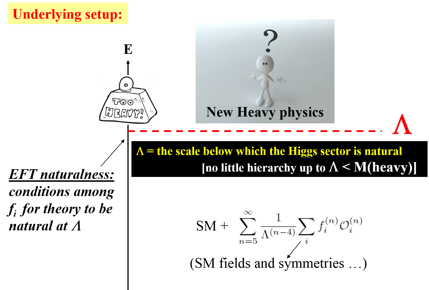
Figure 1: The “EFT Naturalness” setup.

2 Guidelines for EFT

Physics at $E\leq\Lambda$ is assumed to be described by ${\cal L}={\cal L}_{\rm SM}+{\cal L}_{\rm eff}$, where:

$${\cal L}_{\rm eff}=\sum_{n=5}^{\infty}\frac{1}{\Lambda^{(n-4)}}{\sum_{i}f_{i}^{(n)}{\cal O}_{i}^{(n)}}~{}.$$ (2)

and ${\cal O}_{i}^{\left(n\right)}$ are higher dimensional operators ($n$ denotes the dimension and $i$ all other distinguishing labels), which are local, gauge and Lorentz invariant combinations of SM fields and their derivatives. They result from integrating out the heavy degrees of freedom of the heavy NP theory that underlies the SM, and expanding in inverse powers of $\Lambda$ after appropriate renormalization of the SM parameters.

In particular,

• The “light fields” (i.e., at energies $E\leq\Lambda$) are the SM fields.

• The guage-symmetry at $E\leq\Lambda$ is taken to be the SM SU(3)$\times$SU(2)$\times$U(1) gauge symmetry. This is useful for classifying the higher dimensional effective operators [6, 7].

• The underlying NP is assumed to be weakly coupled, renormalizable, obeys gauge-invariance and preserves symmetries of the known dynamics (SM). This is also useful for classifying the higher dimensional effective operators, see e.g., [8].

Three more guiding principles can further simplify/reduce the number of relevant operators (we do not know the precise form of the underlying heavy physics and this leads to ambiguities in selecting the relevant operators for a given process) [6, 7]:

1. The use of equations of motion, also known as the “equivalence theorem”, which is useful when applied to strictly observable quantities. It is therefore not practical for our naturalness study.

2. Integration by parts to dismiss surface terms.

3. Loop Classification of operators (refers to the way they can be generated in the underlying heavy theory): loop-generated (LG) operators versus potentially tree-level generated (PTG) operators.

As it turns out, many operators can be constructed under these conditions, in particular $O(50)$ operators just at dimension 6 [9]. However, as we will show below, only very few can balance the SM’s 1-loop quadratic terms.

3 EFT and the one-loop Higgs mass corrections

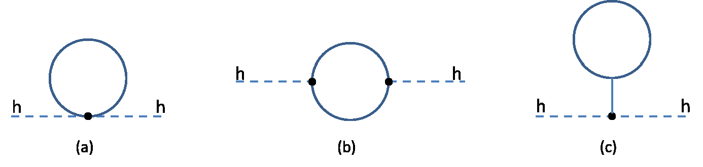
Figure 2: The 1-loop graphs generating $\delta m_{h}^{2}$. The internal lines represent bosons or fermions from either the SM or the heavy NP.

In general, all (SM and NP) one-loop corrections to $m_{h}^{2}$ are generated by the graphs in Fig. 2. In the scenarios we are interested in here, these corrections can be separated into 3 categories:

$\delta m_{h}^{2}({\rm SM})$: When all internal lines are the light SM fields. The contributions from this category are given in Eq. 1.

$\delta m_{h}^{2}({\rm Hvy})$: When all the internal lines are heavy fields of the underlying NP. The contributions from this category are contained in the renormalization of the parameters of the SM that follows upon integration of the heavy particles. This is included in what we denote here as “tree-level” parameters, i.e., $m_{h}^{2}({\rm tree})=m_{h}^{2}({\rm bare})+\delta m_{h}^{2}({\rm Hvy})$ (note that the tree-level mass parameter for $E<\Lambda$ within the EFT prescription need not be the same as the tree-level mass in the full theory, i.e., for $E>\Lambda$).

$\delta m_{h}^{2}({\rm eff})$: When one line is heavy and the other is light (in graphs (b) and (c) in Fig. 2). The contributions in this category are generated by the effective Lagrangian in Eq. 2 and are the ones we are interested in here.

Specifically, our EFT Naturalness approach corresponds to finding those effective interactions that can tame the little hierarchy problem, i.e, leading to $\delta m_{h}^{2}({\rm SM})+\delta m_{h}^{2}({\rm eff})\lesssim m_{h}^{2}$ when $m_{h}\ll\Lambda\leq M$, $M$ being the typical mass scale of the new heavy physics which lies at or above $\Lambda$.

Integrating out the heavy fields with mass $M$, one generates an infinite series of vertices suppressed by inverse powers of $\Lambda$ (recall $\Lambda<M$). This is schematically depicted in Fig. 3, where the effective 4-particle contact vertices on the right hand side correspond to those generated by the effective operators in Eq. 2. Thus, to calculate $\delta m_{h}^{2}({\rm eff})$, we need the set of operators ${\cal O}$ which are not LG and which give the leading contribution to the 1-loop diagrams in Fig. 2(a), where the vertex is generated by the effective operator.

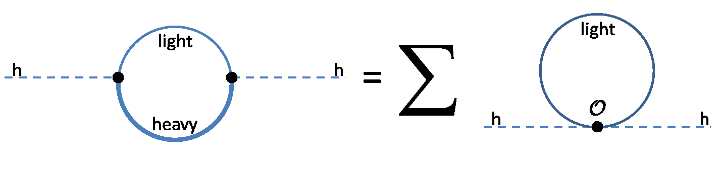
Figure 3: Description of the manner in which the effective Lagrangian Eq. 2 generates graphs in category $\delta m_{h}^{2}({\rm eff})$ defined in the text.

In [5] we have outlined the arguments used to identify all the higher dimensional effective operators that can generate the desired 1-loop $O(\Lambda^{2})$ contributions to $\delta m_{h}^{2}$, and found that they can be of only two types - both types can be derived by integrating out the heavy fields exchanged in the tree-level diagrams depicted in Fig. 4:

• Type I: ${\cal O}$ contains 4 scalar fields, any number of derivatives and is not LG.

• Type II: ${\cal O}$ contains 2 fermions and 2 scalar fields, any number of derivatives and is not LG.

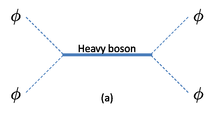
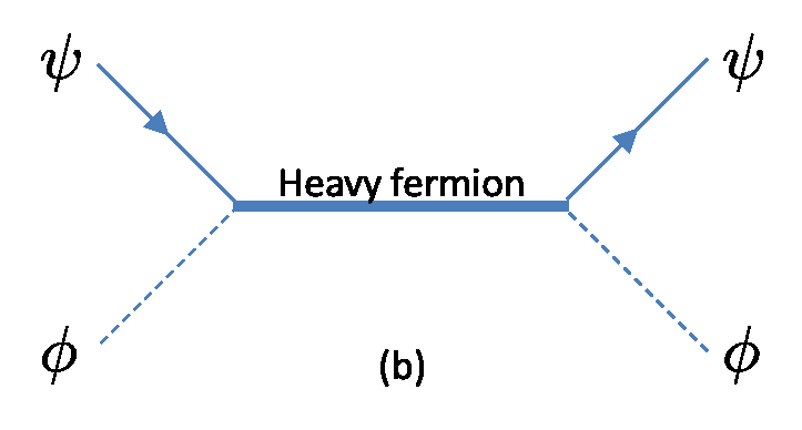
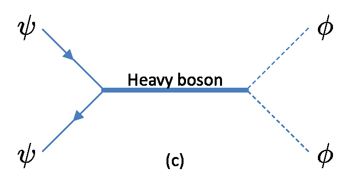
Figure 4: Tree-level graphs that generate the effective operators of type I (diagram a) and II (diagrams b and c), that can produce leading corrections to $\delta m_{h}^{2}$. $\phi$ and $\psi$ denote the SM scalar doublet and fermions, respectively and all vertices are understood to be invariant under SM gauge transformations.

The operators of type I can be further subdivided into those that are generated by tree-level heavy scalar or heavy vector exchanges in diagram Fig. 4(a). The heavy scalar exchanges gives

$${\cal O}_{S}^{\left(2k+4\right)} = \frac{1}{2}|\phi|^{2}\Box^{k}|\phi|^{2}~{},$$

$${\cal O}_{{\bm{\chi}}}^{\left(2k+4\right)} = \frac{1}{2}(\phi^{\dagger}\tau_{I}\phi)D^{2k}(\phi^{\dagger}\tau_{I}\phi)~{},$$

$${\cal O}_{\tilde{\bm{\chi}}}^{\left(2k+4\right)} = \frac{1}{4}(\phi^{\dagger}\tau_{I}\tilde{\phi})D^{2k}(\tilde{\phi}^{\dagger}\tau_{I}\phi)~{},$$ (3)

which correspond to the cases where the heavy scalar is a SM gauge singlet (labeled $S$) or an isotriplet of hypercharge 0 or 1 (labeled ${\bm{\chi}}$ and $\tilde{\bm{\chi}}$, respectively). In the following we denote these heavy scalars collectively by $\Phi$.

Similarly the operators generated by heavy vector exchanges in Fig. 4(a) are

$${\cal O}_{v}^{\left(2k+6\right)}=\frac{1}{2}j_{\mu}\Box^{k}j^{\mu}~{};~{}j^{\mu}\equiv i\phi^{\dagger}D^{\mu}\phi+{\rm H.c.}~{},$$

$${\cal O}_{\tilde{v}}^{\left(2k+6\right)}=\tilde{j}^{\dagger}_{\mu}\Box^{k}\tilde{j}^{\mu}~{};~{}\tilde{j}^{\mu}\equiv i\tilde{\phi}^{\dagger}D^{\mu}\phi~{},$$ (4)

$${\cal O}_{{\bf V}}^{\left(2k+6\right)}=\frac{1}{6}J_{I\mu}D^{2k}J^{\mu}_{I}~{};~{}J^{\mu}_{I}\equiv i\phi^{\dagger}\tau^{I}D^{\mu}\phi+{\rm H.c.}~{},$$

where the labels in Eq. 4 refer to heavy vector isosinglets ($v,\,\tilde{v}$) of hypercharge 0 or 1, respectively, and a heavy vector isotriplet (${\bf V}$) of hypercharge 0. In the following we will collectively denote these heavy vectors by $X$.

Finally, the type II operators are generated in the underlying heavy theory by the graph in Fig. 4(b), which involves an exchange of a heavy fermion $\Psi$ that may or may not be colored and has the same quantum numbers as $\phi\psi$ or $\tilde{\phi}\psi$. That is, $\Psi$ can be an isosinglet, doublet or triplet heavy lepton or quark of hypercharge $y_{\Psi}=y_{\psi}\pm 1/2$ ($y_{r}$ denotes the hypercharge of $r$). These $\Psi$-generated operators are

$${\cal O}^{\left(2k+4\right)}_{\Psi-\psi}=|\phi|^{2}\,\bar{\psi}\left(i\not\!\!D\right)^{2k-1}\psi,\quad(k\geq 1)~{},$$ (5)

where $\psi$ is any SM fermion.

Calculating now the 1-loop quadratic corrections to $m_{h}^{2}$ which are generated by the operators in Eqs. 3, 4 and 5, we obtain [5]:

$$\delta m_{h}^{2}({\rm eff})=-\frac{\Lambda^{2}}{16\pi^{2}}F^{\left(\rm eff\right)}~{},$$ (6)

where

$$F^{\left(\rm eff\right)} = \sum_{k=0}^{\infty}\frac{1}{k+1}\sum_{\Phi}f_{\Phi}^{\left(2k+4\right)}$$ (7)

$$- \sum_{k=0}^{\infty}\frac{1}{k+2}\sum_{X}f_{X}^{\left(2k+6\right)}$$

$$- \sum_{k=1}^{\infty}\frac{(-1)^{k}}{k+1}\sum_{\Psi,\psi}f_{\Psi-\psi}^{\left(2k+4\right)}~{}.$$

with $\Phi=S,~{}{\bm{\chi}},~{}\tilde{\bm{\chi}}$ and $X=v,~{}\tilde{v},~{}{\bf V}$.

4 The “road map” to EFT Naturalness

Let us define the measure for fine-tuning to be $\Delta_{h}\equiv|\delta m_{h}^{2}|/m_{h}^{2}$, where $\delta m_{h}^{2}=\delta m_{h}^{2}({\rm SM})+\delta m_{h}^{2}({\rm eff})$ and $m_{h}^{2}$ is the physical mass, $m_{h}^{2}=m_{h}^{2}({\rm tree})+\delta m_{h}^{2}$. We then have:

$$\Delta_{h}=\frac{\Lambda^{2}}{16\pi^{2}m_{h}^{2}}\left|F^{\left(\rm eff\right)}-8.2\right|~{},$$ (8)

using $24x_{t}^{2}-6\left(2x_{W}^{2}+x_{Z}^{2}+x_{h}^{2}\right)\sim 8.2$ in Eq. 1.

Re-writing the above defined fine-tuning condition as $|m_{h}^{2}({\rm tree})/\delta m_{h}^{2}+1|=1/\Delta_{h}$, we see that a cancellation must occur to a precision of $1/\Delta_{h}$, so that a larger $\Delta_{h}$ corresponds to a less natural theory. Inspection of Eq. 8 shows that, for naturalness to be restored at $\Lambda$, the cancellation must occur among the 1-loop contributions (i.e., leading to a natural $m_{h}({\rm tree})\sim m_{W}$) or else there should be a correlation between $m_{h}({\rm tree})$ and $\delta m_{h}$, in which case $m_{h}({\rm tree})\sim m_{W}$ will require fine-tuning.

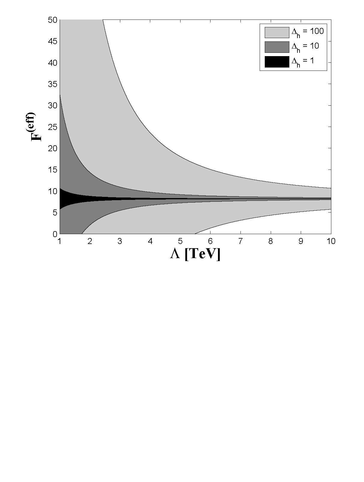
Figure 5: Regions in the $F^{\left(\rm eff\right)}-\Lambda$ plane where naturalness can be restored with no fine-tuning ($\Delta_{h}=\delta m_{h}^{2}/m_{h}^{2}=1$, in black) and with fine-tuning at the level of 10% (dark gray) and 1% (light gray), corresponding to $\Delta_{h}=\delta m_{h}^{2}/m_{h}^{2}=10$ and 100, respectively. See also text.

Therefore, a theory (i.e., $F^{\left(\rm eff\right)}$) for which $\Delta_{h}=1$ is natural, while one with $\Delta_{h}=10(100)$ suffers from fine-tuning of (no worse than) 10%(1%). In Fig. 5 we plot regions in the $F^{\left(\rm eff\right)}-\Lambda$ plane that correspond to NP theories which are natural (i.e., enclosed within the $\Delta_{h}=1$ region) and those that suffer from fine-tuning of no worse than 10% and 1%, corresponding to $\Delta_{h}=10$ and $\Delta_{h}=100$, respectively. We find, for example, that theories for which $8.17\lesssim F^{\left(\rm eff\right)}\lesssim 8.23$ are natural at $\Lambda\sim 10$ TeV, while theories with $7.95\lesssim F^{\left(\rm eff\right)}\lesssim 8.45$ or $5.73\lesssim F^{\left(\rm eff\right)}\lesssim 10.67$ will suffer from 10% or 1% fine-tuning, respectively, at $\Lambda\sim 10$ TeV. Clearly, if the NP scale for EFT Naturalness is $\Lambda\sim 5$ TeV, then a much wider range of theories are allowed if one is willing to tolerate 1% fine-tuning, in particular those giving $0\>\raisebox{-2.15277pt}{$\stackrel{{\scriptstyle\textstyle<}}{{\sim}}$}\>F^{\left(\rm eff\right)}\>\raisebox{-2.15277pt}{$\stackrel{{\scriptstyle\textstyle<}}{{\sim}}$}\>18$.

Finally, we emphasize that, for a specific heavy NP model, $F^{\left(\rm eff\right)}$ will be a dimensionless function of the NP parameters and $\Lambda$, such as the ratio $\Lambda/M$ (where $M$ denotes one of the heavy particle masses, see next section). Thus, $F^{\left(\rm eff\right)}$ is in general cutoff dependent, so that the cancellation conditions will depend on $\Lambda$ as well. Our requirement that $\Lambda$ be the scale below which the SM little-hierarchy problem is solved is consistent within our EFT Naturalness scenario because of the requirement $M>\Lambda$.

5 Less ignorance: insight for a natural heavy NP

Let us now examine the general content and properties of the heavy NP that can generate the effective operators in Eqs. 3, 4 and 5 at tree-level, and find the EFT Naturalness conditions within these theories. In particular, we can calculate the cutoff-dependent coefficients $f_{\Phi}^{\left(2k+4\right)}$, $f_{X}^{\left(2k+6\right)}$ and $f_{\Psi-\psi}^{\left(2k+4\right)}$ in Eq. 7, in terms of the parameters (masses and couplings) of the underlying NP theory.

The general form of the potentially natural NP which contains the relevant interactions of the heavy scalars ($S,~{}{\bm{\chi}},~{}\tilde{\bm{\chi}}$) to $\phi^{2}$, of the heavy vectors ($v,~{}\tilde{v},~{}{\bf V}$) and of the heavy fermions ($\Psi$) to $\psi\phi$ are [5]:

$$\Delta{\cal L}_{\Phi} = u_{S}S|\phi|^{2}+u_{\bm{\chi}}\phi^{\dagger}{\bm{\chi}}\phi+\frac{1}{2}\left(u_{\tilde{\bm{\chi}}}\tilde{\phi}^{\dagger}\tilde{\bm{\chi}}\phi+{\rm H.c}\right)~{},$$ (9)

$$\Delta{\cal L}_{\Psi} = \sum_{\Psi,\,\psi}\left(y_{\Psi-\psi}\bar{\psi}\Psi\phi+{\rm H.c}\right)~{},$$ (10)

$$\Delta{\cal L}_{X} = g_{v}v_{\mu}j^{\mu}+g_{\bf V}{\bf V}_{\mu}\cdot{\bf J}^{\mu}+\left(g_{\tilde{v}}{\tilde{v}}_{\mu}{\tilde{j}}^{\mu}+{\rm H.c.}\right)~{},$$ (11)

where the currents $j,~{}\tilde{j}$ and J (with components $J_{I}$) are defined in Eq. 4.

Using Eq. 11 to calculate the diagrams in Fig. 4 in the limit that the masses are larger than the typical momentum transfer involved, we find:

$$f_{\Phi}^{\left(2k+4\right)}(\Lambda) = \left|\frac{u_{\Phi}}{M_{\Phi}}\right|^{2}\left(\frac{-\Lambda^{2}}{M_{\Phi}^{2}}\right)^{k}~{},$$

$$f_{\Psi-\psi}(\Lambda)^{\left(2k+4\right)} = \frac{1}{2}I_{\Psi}|y_{\Psi-\psi}|^{2}\left(\frac{\Lambda^{2}}{M_{\Psi}^{2}}\right)^{k}~{},$$

$$f_{X}^{\left(2k+6\right)}(\Lambda) = I_{X}|g_{X}|^{2}\left(\frac{-\Lambda^{2}}{M_{X}^{2}}\right)^{k+1}~{},$$ (12)

where $I_{\zeta}=1,\,2,\,3$ when the field $\zeta$ is an isosinglet, doublet or triplet, respectively, and $M_{\Phi,\Psi,X}\gtrsim\Lambda$ are the masses of the heavy scalars, fermions and vectors, respectively.

Thus, matching the effective theory at $\Lambda$ and using the definition of $F^{\left(\rm eff\right)}$ in Eq. 7, we obtain the 1-loop corrections to the Higgs mass in terms of the parameters of the new heavy physics (i.e., from $\Delta{\cal L}_{NP}=\Delta{\cal L}_{\Phi}+\Delta{\cal L}_{\Psi}+\Delta{\cal L}_{X}$):

$$F^{\left(\rm eff\right)}(\Lambda) = \sum_{\Phi}\frac{|u_{\Phi}|^{2}}{M_{\Phi}^{2}}A\left(\frac{\Lambda^{2}}{M_{\Phi}^{2}}\right)$$ (13)

$$+ \frac{1}{2}\sum_{\Psi,\psi}I_{\Psi}|y_{\Psi-\psi}|^{2}\left[1-A\left(\frac{\Lambda^{2}}{M_{\Psi}^{2}}\right)\right]$$

$$+ \sum_{X}I_{X}|g_{X}|^{2}\left[1-A\left(\frac{\Lambda^{2}}{M_{X}^{2}}\right)\right]~{},$$

where $A(x)=\ln(1+x)/x$, so that $1>A(x)\geq 0$, from which it follows that $F^{\left(\rm eff\right)}>0$.

The upshot of this phenomenological study of EFT Naturalness is that, given the masses and couplings of the new heavy states (heavy fermions, scalars and/or vectors), we can derive the scale $\Lambda$ - below which the corresponding underlying theory is natural or has a certain degree of fine-tuning. In particular, the EFT Naturalness scale can be written as $\Lambda=\Lambda(\Delta_{h},g_{NP},M_{NP})$, where $g_{NP}$ and $M_{NP}>\Lambda$ are the couplings and masses of the new heavy states. Naturality at $\Lambda$ (i.e., below which the corresponding extension to the SM is natural) is, therefore, given by $\Lambda=\Lambda(\Delta_{h}=1,g_{NP},M_{NP})$.

To illustrate the above, let us consider the simplest model for EFT Naturalness, where the SM is minimally extended by one real scalar singlet $S$, with a mass $M_{S}$ and a super-renormalizable scalar coupling $u_{S}$ in Eq. 11, i.e., the case where ${\cal L}={\cal L}_{SM}+u_{S}S|\phi|^{2}$. In particular, we wish to find the scale $\Lambda$ below which this one singlet extension of the SM is natural? As we have shown above, this scale will depend on the mass ($M_{S}$) and coupling ($u_{S}$) of the singlet $S$ to $\phi^{2}$, i.e., $\Lambda=\Lambda(1,u_{S},M_{S})$.

From Eq. 13 we can obtain the 1-loop contribution of a heavy scalar singlet to the Higgs mass:

$$\delta m_{h}^{2}({\rm eff};S)=-\frac{|u_{S}|^{2}}{16\pi^{2}}\ln\left(1+\frac{\Lambda^{2}}{M_{S}^{2}}\right)~{},$$ (14)

so that the overall 1-loop correction to the Higgs mass in this model is (keeping only the top-quark loop for the SM contribution):

$$\delta m_{h}^{2} = \delta m_{h}^{2}({\rm SM})+\delta m_{h}^{2}({\rm eff};S)$$ (15)

$$\approx \frac{\Lambda^{2}}{16\pi^{2}}\cdot\left(24\frac{m_{t}^{2}}{v^{2}}-\frac{|u_{S}|^{2}}{\Lambda^{2}}\ln\left(1+\frac{\Lambda^{2}}{M_{S}^{2}}\right)\right)~{}.$$

In Fig. 6 we plot the regions in the $\Lambda/u_{S}-\Lambda/M_{S}$ plane which correspond to $\Delta_{h}=1,~{}10$ and 100, for a fixed NP naturalness scale of either $\Lambda=5$ TeV or $\Lambda=10$ TeV. Note that $0<\Lambda/M_{S}\leq 1$ (i.e., $M_{S}\geq\Lambda$ for the EFT prescription to be valid, see discussion above). Thus, we can find from Fig. 6 the values of ($M_{S},u_{S}$) for which the one scalar singlet extension of the SM can restore naturalness in the Higgs sector up to $\Lambda=5$ TeV or $\Lambda=10$ TeV. For example, as marked on the plot, if $M_{S}\sim 12$ TeV and $u_{S}\sim 36$ TeV, then the Higgs sector of this model is natural up to $\Lambda=5$ TeV, while it will require fine-tuning at the level of $\sim 4\%$ for $\Lambda\sim 10$ TeV, i.e., if no additional new physics appear below $\sim 10$ TeV. This result should be interpreted as follows: the one scalar singlet extension of the SM with this choice of parameters (i.e., $M_{S}\sim 12$ TeV and $u_{S}\sim 36$ TeV) is natural up to scales $\sim 5~{}\hbox{TeV}$ (an order of magnitude improvement over the pure SM).

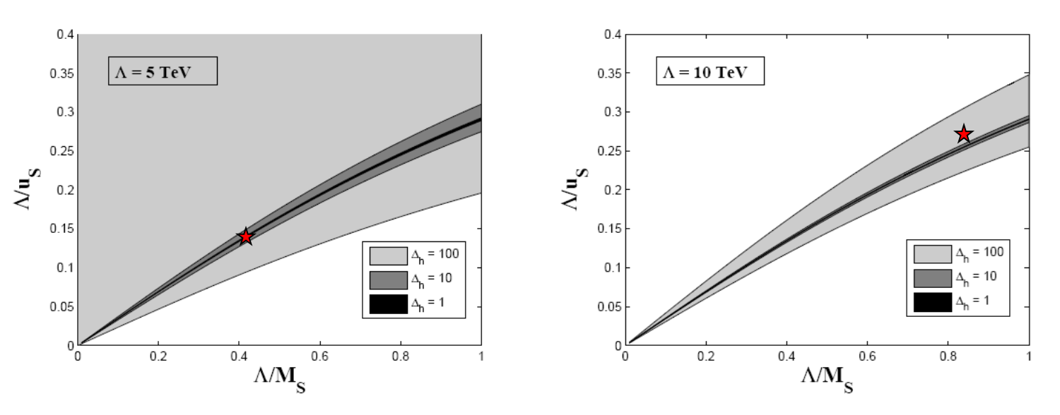
Figure 6: Regions in the $({\Lambda}/{u_{S}})-({\Lambda}/{M_{S}})$ plane, for $\Lambda=5$ TeV (left) and $\Lambda=10$ TeV (right), where naturalness can be restored with no fine-tuning ($\Delta_{h}=\delta m_{h}^{2}/m_{h}^{2}=1$, in black) and with fine-tuning at the level of 10% (dark gray) and 1% (light gray), corresponding to $\Delta_{h}=\delta m_{h}^{2}/m_{h}^{2}=10$ and 100, respectively. The red stars indicate the case where the scalar singlet has a mass $M_{S}=12$ TeV and a super-renormalizable coupling $u_{S}=36$ TeV.

6 Constraints from current data

In [5] we have studied the constraints that the present data imposes on our EFT Naturalness operators. We found that these operators can cause 2 types of effects that need to be considered: a shift to the $\rho$-parameter and a shift of the SM Higgs couplings to the SM fermions and gauge-bosons, which, therefore, needs to be confronted with the measured production and decay rates of the recently discovered 125 GeV Higgs state.

We have found that while in the latter case (i.e., the deviations of the Higgs production and decay rates) no useful limit can be obtained, the well measured value of the $\rho$-parameter imposes a bound of $\Lambda\>\raisebox{-2.15277pt}{$\stackrel{{\scriptstyle\textstyle>}}{{\sim}}$}\>10$ TeV on the scale of the operators involving the heavy scalar triplets and heavy vector exchanges.

7 Collider signals of EFT Naturalness

Let us briefly discuss the potential collider signals of our EFT Naturalness operators, or equivalently, of the NP that can restore naturalness at energy scales which are accessible to current and future high energy colliders.

As for the heavy singlet example discussed above, it is expected to have a small mixing with the CP-even component of the SM Higgs doublet (see e.g., [10, 11]) and is, therefore, unlikely to be detected at the 14 TeV LHC; whether it is produced through Higgs bremshtralung $h_{SM}^{\star}\rightarrow h_{SM}S$ or in the s-channel, leading e.g., to $pp\rightarrow S\rightarrow h_{SM}h_{SM}$ [12].

On the other hand, in the more general case (where the heavy new physics includes new heavy triplet bosons and/or new heavy fermions), the experimental signals of the new physics which can potentially be responsible for EFT Naturalness may be searched for in Higgs pair production, for example in $VV\rightarrow hh$ ($V=W,~{}Z$) due to an s-channel exchange of an off-shell heavy boson and in $\bar{\psi}\psi\rightarrow hh$ ($\psi$ is a SM lepton or quark) due to a t-channel exchange of an off-shell heavy fermion $\Psi$. Another interesting signature of the potential role that a heavy fermion may have in curing the little hierarchy problem of the SM, is the production of Higgs+quark(jet) or Higgs+lepton, via its (off-shell) coupling $\Psi^{\star}\rightarrow h\psi$.

8 Summary

We have used EFT techniques to analyse naturalness in the SM Higgs sector in a model independent way, by calculating the 1-loop contributions to the SM Higgs mass, generated by a set of higher dimensional effective operators. These higher dimensional effective operators correspond to exchanges of heavy fermions, scalars and gauge-bosons in generic underlying renormalizable gauge theories with a typical mass scale $M\geq\Lambda$, where $\Lambda$ is defined to be the scale below which these theories are natural.

This framework allows us to find the conditions under which the 1-loop corrections to $m_{h}$ from the new heavy physics can balance those created by SM loop effects up to the naturalness scale $\Lambda$, a condition we denote by “EFT Naturalness”. Our EFT Naturalness conditions, therefore, depends on the heavy particle spectrum and its interactions with the SM Higgs and it proved to be useful for acquiring insight regarding the underlying heavy theories that can address the naturalness problem of the SM, in particular, for deriving relations among the parameters of the underlying NP theory.

References

- [1] S. Chatrchyan et al., [CMS Collaboration], Phys. Lett. B716, 30 (2012); G. Aad et al., [ATLAS Collaboration], Phys. Lett. B716, 1 (2012).
- [2] B. Grzadkowski and J. Wudka, Phys. Rev. Lett. 103, 091802 (2009).
- [3] A. Drozd, B. Grzadkowski and J. Wudka, JHEP 1204, 006 (2012).
- [4] N. Craig, C. Englert and M. McCullough, Phys. Rev. Lett. 111, 121803 (2013); S. El Hedri and A. Hook, JHEP 1310, 105 (2013); M. Farina, M. Perelstein and N. Rey-Le Lorier, arXiv:1305.6068 [hep-ph]; A. de Gouvea, D. Hernandez and T.M.P. Tait, arXiv:1402.2658 [hep-ph].
- [5] S. Bar-Shalom, A. Soni and J. Wudka, arXiv:1405.2924 [hep-ph].
- [6] C. Arzt, M.B. Einhorn and J. Wudka, Nucl. Phys. B433, 41 (1995).
- [7] M. B Einhorn and J. Wudka, Nucl. Phys. B876, 556 (2013).
- [8] E. E. Jenkins, A. V. Manohar and M. Trott, JHEP 1309, 063 (2013).
- [9] B. Grzadkowski, M. Iskrzynski, M. Misiak and J. Rosiek, JHEP 1010, 085 (2010).
- [10] S. Profumo, M.J. Ramsey-Musolf, C.L. Wainwright and P. Winslow, arXiv:1407.5342 [hep-ph].
- [11] G.M. Pruna and T. Robens Phys. Rev. D88, 115012 (2013).
- [12] See e.g., J.M. No and M. Ramsey-Musolf, Phys. Rev. D89, 095031 (2014).