Void asymmetries in the cosmic web: a mechanism for bulk flows

Abstract

Bulk flows of galaxies moving with respect to the cosmic microwave background are well established observationally and seen in the most recent $\Lambda$CDM simulations. With the aid of an idealised Gadget-2 simulation, we show that void asymmetries in the cosmic web can exacerbate local bulk flows of galaxies. The Cosmicflows-2 survey, which has mapped in detail the 3D structure of the Local Universe, reveals that the Local Group resides in a “local sheet” of galaxies that borders a “local void” with a diameter of about 40 Mpc. The void is emptying out at a rate of 16 km s^-1 Mpc^-1. In a co-moving frame, the Local Sheet is found to be moving away from the Local Void at $\sim 260$ km s^-1. Our model shows how asymmetric collapse due to unbalanced voids on either side of a developing sheet or wall can lead to a systematic movement of the sheet. We conjectured that asymmetries could lead to a large-scale separation of dark matter and baryons, thereby driving a dependence of galaxy properties with environment, but we do not find any evidence for this effect.

1 Introduction

The physics of baryons across the universe is the grandest of all environmental sciences. This drama is played out against a backdrop of evolving dark matter structure from the Big Bang to the present day. Cold dark matter (CDM) simulations without baryons reveal a universe that looks structurally different from the observed universe defined by its baryons. The most recent CDM simulations that include baryons and hydrodynamics emphasise how little we know of baryonic processes throughout cosmic time (Schaye et al 2014; Vogelsberger et al 2014).

This meeting honours the 100th year since the birth of Y.B. Zel’dovich. In 1977, Tallinn, Estonia was the site of the first great conference on large-scale structure. Over the past week, much of the discussion centred on where next for studies of the cosmic web and galaxy redshift surveys. An interesting question is how the ratio of baryons to dark matter by mass ($\langle f_{b}\rangle$) varies across large-scale structure. Non-standard models do exist which predict baryon to dark matter variations (Malaney & Mathews 1993; Gordon & Lewis 2003). Variations in $\langle f_{b}\rangle$ of order 10% lead to only few percent variations in the matter power spectrum, but could conceivably lead to observable differences in some local galaxy properties (Nichols & Bland-Hawthorn 2013). In clusters, the baryon fraction approaches the universal average $\langle f^{o}_{b}\rangle\approx 15.5\%$ (Planck) with small scatter (Sun et al 2009). For most galaxies in groups, this ratio is more uncertain largely because the warm-hot gas phases are very difficult to detect. In some instances, the majority of the missing baryons may be in a warm circumgalactic medium (Tumlinson et al 2011; Shull et al 2012).

The next generation of large-scale galaxy surveys will seek to associate more of a galaxy’s properties with its large-scale environment (Croom et al 2012; Bundy et al 2014; Bland-Hawthorn 2014). While the distinction between clusters and the field is well defined, the dependence of a galaxy’s properties on a more graded local density has been hard to establish (e.g. Blanton & Moustakas 2009; Metuki et al 2014). The effects appear to exist only weakly, if at all. These include a weak dependence of the fundamental plane with environment, scatter in the mass-metallicity relation that correlates with environment (Cooper et al 2008), and mean star formation rates showing a trend with environment (Lewis et al 2002; Gomez et al 2003). The weakness of these trends may arise from any of the following: (i) the difficulty of defining environment; (ii) the wrong galaxy parameters are being explored; (iii) a strong local dependence does not exist in nature.

In light of recent simulations where void-void imbalances are observed to push material around (Pichon et al 2011; Codis et al 2012), we look more closely at the prospect of baryon-dark matter variations. While the effects look strong in our 1D toy model, they are essentially non-existent in 3D. But what we do find is a barycentric drift of the collapsed sheet and a possible mechanism for bulk flows in galaxies (e.g. Rubin et al 1976; Burstein et al 1990; Tully et al 2008).

In §2, we introduce our 1D toy model for asymmetric collapse that suggests a strong separation of dark matter and baryons. We investigate this idea further in §3 with a cosmologically motivated 3D model using Gadget-2. In §4, we conclude that there is no general case for baryon-dark matter separation on megaparsec scales, but we establish an interesting mechanism for bulk flows in the presence of void asymmetries in the cosmic web.

2 Toy model

Can baryons and dark matter separate on megaparsec scales? The short answer is yes in specific cases, for example, the Bullet Cluster (e.g. Mastropietro & Burkert 2008) where two massive clusters have passed through each other sweeping out the baryons in both systems. This provides us with our initial motivation for modelling the Local Sheet. To illustrate how the Local Sheet can be kinematically offset from the Local Void, initially, we reduce the the dynamics of a forming sheet to a one-dimensional problem (cf. Melott 1983). Before exploring a cosmologically motivated N-body simulation in co-moving coordinates, we develop a toy model using the “infinite sheets” approximation (Binney & Tremaine 2008, hereafter BT08). This approach has a long history dating back to theoretical work in plasma physics (Eldridge & Feix 1963) although its relevance to structure formation has been demonstrated in numerous papers (Yamashiro et al 1992). An up-to-date discussion is given by Teles et al (2011) who call for the sheets approximation to be explored in a cosmological context, as we do here.

We simulate the formation and evolution of the Local Sheet using thin sheets of dark matter and a matching set of (initially cospatial) sheets made of gas. The dark matter is treated as collisionless while the gas is assumed to undergo inelastic collisions. In the expanding universe, dark matter and baryons turn around and begin to collapse towards a local density perturbation. At turnaround, when no sheet crossing has occurred, the evolution is described by linear theory. But during the collapse phase, the sheets start to cross each other, and the evolution becomes non-linear. We start the simulation just after turn around. Initially we treat the symmetric case where the sheet separations have a Gaussian distribution in the normal ($x$-axis) direction. The gas and dark matter sheets are assumed to extend to infinity in the $y-z$ plane such that the force exerted by any sheet is constant at any point

The equation of motion for the sheets along the $x$ axis is given by

$$\ddot{x}=2\pi G\int_{-\infty}^{\infty}{\rm Sgn}(x^{\prime}-x)\sigma(x^{\prime})dx^{\prime}$$ (1)

or equivalently

$$\ddot{x}=f(x)=2\pi G(2\Sigma(>x)-\Sigma_{\rm tot})$$ (2)

where $\Sigma(>x)$ is the cumulative surface density and it is assumed that $\Sigma(<x)+\Sigma(>x)=\Sigma_{\rm tot}$. For a discretized system, one can think of $2N+1$ sheets distributed in space with $i$-th sheet having surface density $m_{i}$. $N$ must be large enough to render the system “collisionless” as discussed by Yamashiro et al (1992). The mass of the $i$-th sheet is assumed to be distributed evenly between $(x_{i-1}+x_{i})/2$ and $(x_{i+1}+x_{i})/2$. Here we assume that all dark matter sheets have the same constant surface density; the gas sheets also have a constant surface density defined to be a factor of 10 lower ($\langle f_{b}\rangle$=0.1) than for the dark matter. In our analysis, we set $G=1$ and choose $\Sigma_{\rm tot}=\int\sigma(x)dx=1/(2\pi)$.

Initial conditions. Let $\sigma(\xi)$ ($-1<\xi<1$) be the initial density distribution at shortly after the Big Bang ($t=0$). If no shell crossings have happened since the Big Bang, the acceleration is constant and is given by

$$a(\xi)=-2\pi G\int_{-1}^{1}{\rm Sgn}(\xi^{\prime}-\xi)\sigma(\xi^{\prime})d\xi^{\prime}.$$ (3)

Let $v(\xi)=v_{\rm tot}\xi$ be the initial velocity field. The collapse time is given by

$$t_{\rm collapse}=-\frac{2v(\xi=1)}{a(\xi=1)}=\frac{v_{\rm tot}}{\pi G\Sigma_{\rm tot}}$$ (4)

The position and velocity at a later time $\tau$ is given by

$$x(\xi,\tau)=v_{\rm tot}\xi\tau+\frac{a(\xi)\tau^{2}}{2}\\ \ v(\xi,\tau)=v_{\rm tot}\xi+a(\xi)\tau.$$ (5)

After BT08, we set $v_{\rm tot}=0.75$, which at $\tau=1$ gives max($v$)=max($x$)=0.25.

Let the initial sheet distribution be given by a function of form

$$\sigma(\xi)=\frac{k}{1-a{\rm cos}(b\pi\xi)}{\rm\ \ },-1<\xi<1.$$ (6)

Using $\int_{-1}^{1}\sigma(\xi)d\xi=1$, the normalization constant is given by

$$k=\frac{\pi b\sqrt{1-a^{2}}}{4{\rm tan^{-1}}((1+a){\rm tan}(b\pi/2)/\sqrt{1-a^{2}})}$$ (7)

To sample such a distribution we use the method of inverse transform sampling. Let $F(>\xi)$ be the cumulative distribution, then for $u$ uniformly sampled between 0 and 1, the $\xi$ is given by

$$\xi = F^{-1}(u)$$ (8)

$$= \frac{2}{b\pi}{\rm tan}^{-1}\left[\frac{\sqrt{1-a^{2}}}{1+a}{\rm tan}\left(\frac{(b\pi\sqrt{1-a^{2}})}{2k}(u-0.5)\right)\right]$$ (9)

Here we set $a=0.3$ and $b=0.3$ (BT08).

For the asymmetric case, the density is defined as follows

$$\Sigma^{\prime}(\xi)=\left\{\begin{array}[]{rl}\Sigma(\xi)&\mbox{ if $\xi<0$}\\ 2\Sigma(2\xi)&\mbox{ if $\xi>0$}\end{array}\right.$$

This is achieved by setting $\xi=\xi/2$ for $\xi>0$. The position and velocities are calculated as in the symmetric case. Note for the region $\xi>0$, the collapse time now decreases by a factor of two.

To evolve a system of sheets, we use the kick-drift-kick algorithm. For fixed time step $\Delta t$ this is given as

$$v_{i} = v_{i}+f(x_{i})\Delta t$$ (10)

$$x_{i} = x_{i}+v_{i}\Delta t$$ (11)

$$v_{i} = v_{i}+f(x_{i})\Delta t$$ (12)

A time step of $\Delta t=10^{-4}\tau$ was employed in all runs. The results were checked for convergence: choosing a lower time step did not yield any difference in results. For collisionless sheets, it is sufficient to just evolve the as shown above, but for gas one has to put in additional physics. We assume the gas sheets undergo fully inelastic collisions, which conserve mass and momentum, but not energy. The prescription to simulate this is as follows. In a given time step, we identify a contiguous set of gas sheets that criss-cross each other as predicted by the equation of motion. This can be easily accomplished by sorting the sheets before and after advancing. If $L_{1}$ and $L_{2}$ are lists that contain sorted indices, then two gas sheets are set to cross if $L_{1}-L_{2}$ is non-zero. Two (or more) gas sheets that are set to cross in the next step are joined to form a single particle whose position is given by the center of mass of the sheets in the set. The momentum and mass is assumed to be conserved.

Figure 1: Evolution in phase space of parallel infinite sheets. The time of the Big Bang is $-\tau$ and the units of time are in units of time $\tau$. (Left) Dark matter only, symmetric perturbation. (Right) Dark matter $+$ gas, asymmetric perturbation.

In our first test, we run a simulation with dark matter. In Fig. 1 (left), we accurately recover Fig. 9.14 in BT08. The curves are smooth and continuous in phase space, which tells us that the time integration is working correctly. We now study the evolution of sheets when both dark matter and gas are present together. We consider both the symmetric and asymmetric perturbations where the functional form of the perturbation is given by Equation (6).

Symmetric perturbation. The first panel in Fig. 2 (Left) shows the variation of the center of mass position and center of mass velocity with time; these are shown separately for gas ($x_{\rm gas}$, $v_{\rm gas}$) and dark matter ($x_{\rm DM}$, $v_{\rm DM}$). The middle panel shows the dispersion $\sigma_{x}$ or spread of the sheets along the $x$-axis. The dark matter sheets show oscillatory behaviour while the gas sheets stick after the first crossing. The bottom panel shows the variation in the mean kinetic energy. The kinetic energy of the gas sheets is assumed to be lost to internal energy within the sheets through shock heating. We explored different baryon fractions from $f_{b}=0.01$ to $f_{b}=0.1$. A larger value of $f_{b}$ increases the time required by dark matter to achieve the second turnaround and collapse. We observe that there is no offset between the center of mass of the dark matter and the gas $-$ all of the lines are overlaid (see top left panel).

Asymmetric perturbation. In Fig. 2, we compare our asymmetric collapse model with the symmetric case. Clear differences are evident. The asymmetric distribution of sheets leads to an initial (non-zero) offset in the velocity centroid of the gas and dark matter. As the collapse proceeds, the gas becomes progressively separated from the dark matter. The dark matter starts to exert a force on the gas and, at a later stage, gas tries to move towards the dark matter’s centre of mass. A larger value of $f_{b}$ increases the spatial offset and delays the time required by the baryons to turn around and fall towards the dark matter. The kinematic offset between the gas and dark matter is exaggerated here because of the artificial asymmetry built into our model. Now we turn our attention to sheet collapse in a 3D cosmological context.

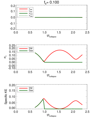
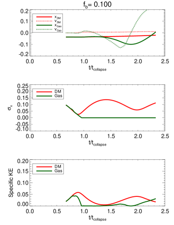
Figure 2: Evolution of position and velocity of the center of mass of dark matter, gas and the whole system. The middle panel shows the dispersion of sheets in space and the bottom panel shows the specific kinetic energy. The simulation explores the evolution of a symmetric perturbation (Left) and an asymmetric perturbation (Right). In the top left figure, all of the curves are overlaid.

3 Simulation with Gadget-2 in a cosmological context

3.1 Vacuum boundaries

We explore a collapsing sheet where the perturbation takes the form

$$\rho(z)=A\cos(2\pi z/L).$$ (13)

Note that the collapse is now along the $z$ axis. The amplitude $A$ was selected so that $\delta\rho/\rho=1$ at redshift ${\cal Z}={\cal Z}_{\rm collapse}=2$. This perturbation was evolved using linear theory till ${\cal Z}={\cal Z}_{\rm start}=6.6$, the point from where the simulation starts. To set up the perturbation, the particles were initially distributed uniformly in a box of size $L=10$ Mpc h^-1 and a spherical region was cut from this. We adopt a $\Omega_{m}=1$ and $\Omega_{b}=0.05$ co-moving cosmology. Here we use $N=32^{3}$ particles for the dark matter, and the same for the gas. The displacement field corresponding to the perturbation was calculated, viz.

$$S(z)={{-2\pi z}\over{LA}}\sin(2\pi z/L)$$ (14)

and the particles were accordingly displaced from the uniform distribution to generate the perturbation. The time integration was done in co-moving coordinates using Gadget-2. The results of the symmetric collapse (Fig. 3) are in good agreement with Dekel (1983).

The asymmetric case was set up by increasing the displacement field by a factor of two for $z>0$. In Fig. 3, we show the initial $z-v_{z}$ and density distribution of the particles. At ${\cal Z}=0.9$, there is a bump in the density distribution of dark matter particles at around 400 kpc h^-1. This behaviour is not seen in the gas. The gas centre of mass shows a slight displacement with respect to dark matter similar to our idealized 1D simulation, but the displacement is very small and is less than the softening parameter ($\epsilon=12.5$ kpc h^-1). An $N=64^{3}$ simulation with $\epsilon=6.25$ kpc h^-1 also shows similar behaviour. We note that the amount of displacement in the 1D case is much larger than for the 3D set-up in physically motivated co-moving coordinates.

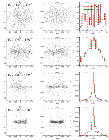
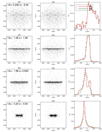
Figure 3: The distribution of particles in $x-z$ space as a function of time for a 10 Mpc h^-1 simulation with a symmetric cosine perturbation (left) and an asymmetric perturbation (right) along the $z$-direction. These are evolved with Gadget-2 with no gas cooling. The perturbation is imposed over a uniform sphere.

3.2 Periodic Boundaries

In earlier simulations, a plane wave perturbation was imposed on a uniform sphere and the asymmetry function had a discontinuity at $z=0$. We now employ a periodic box and use a better asymmetry function. The symmetric perturbation is a cosine function and we now add a $\tanh$ function to make it asymmetric (see §3.3), such that

$$\delta(z)=A\left[\left(1+\tanh\left(\frac{z2\pi}{\lambda\alpha}\right)\right)\left(1+\cos\left(\frac{z2\pi}{\lambda}\right)\right)-1\right]$$ (15)

For $\alpha\gg 1$, this reduces to the plane wave form $\delta(z)=A\cos(2\pi z/\lambda)$. The degree of asymmetry is controlled by the shape parameter $\alpha$. The smaller the value of $\alpha$, the higher the asymmetry. The functional form for different $\alpha$ is shown in Fig. 4 (Left). The function and its first derivative are continuous across the boundary of the box; more details are given in § 3.3.

We simulate 7 different types of perturbation: one is a symmetric cosine wave; the others use an asymmetry factor $\alpha=100,10,1,0.5,0.25$ and $0.1$. These were simulated with and without cooling. A smoothing length of 12.5 kpc h^-1 was used. $N=32^{3}$ particles were used once again for each constituent in the simulation and the cosmology adopted is $\Omega_{m}=1$ and $\Omega_{b}=0.05$. The amplitude of the perturbation was set so as to make the cosine perturbation collapse at redshift ${\cal Z}_{\rm collapse}=2$. A starting redshift of ${\cal Z}_{\rm start}=6.6$ was used. These last two parameters are the same as in our first Gadget-2 run with vacuum boundary conditions. Here we only show results for the symmetric case and with $\alpha=1$, $0.5$ and $0.25$.

In Fig. 5, we show the density distribution of the dark matter and gas along the $z-$axis (in co-moving coordinates). The type of perturbation and details about cooling are given on top of each figure. To simulate gas cooling, we set an upper bound on the temperature at $1000K$. The results with and without cooling are very similar. A notable feature is the occurrence of spikes at the edges due to the piling up of particles at turnaround after shell crossing. This was also noticed by Dekel (1983) in his simulations. The gas is not so able to criss-cross and thus forms a central peak. The fact that, even with cooling, the dispersion of the gas does not diminish is interesting. The gas appears to expand as the DM potential becomes shallower which may be why cooling does not seem to have a great effect on the final distribution of gas. For the asymmetric perturbation, the behaviour is similar except for the fact that the spikes are asymmetric.

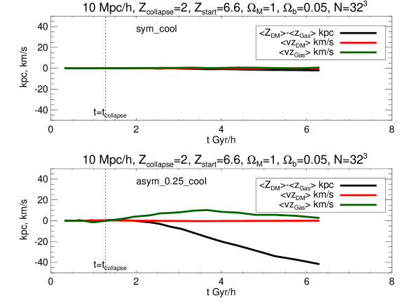
Figure 6: Evolution of the position and velocity (proper) of center of mass of dark mater and gas for a 10 Mpc h^-1, $N=32^{3}$ simulation with periodic boundaries. (Top) Symmetric case with cooling; (Bottom) Asymmetric perturbation $\alpha=0.25$ with cooling. Even under large asymmetry, the gas to a good approximation tracks the dark matter.

In the panels of Fig. 6, we plot as a function time the center of mass offset between gas and dark matter– defined as $\Delta_{z}=\langle z_{DM}\rangle-\langle z_{Gas}\rangle$. The velocity of center of mass of gas and dark matter is also shown on the same panel. All quantities in these set of figures are in physical coordinates, i.e. physical length and physical peculiar velocity (without hubble flow).

For $\alpha<0.5$, i.e., large asymmetry, one can see that the offset $\Delta_{z}$ reaches to about $40$ kpc at redshift zero. The dispersion in $z$ is around $1000$ kpc, or an offset that is about 4% of the dispersion. Overall, the offset and velocity of the center of mass are quite small. Nevertheless, it is interesting to explore the cause of the shift. First thing to note is that the offset occurs only after the collapse of the perturbation, i.e., after shell crossing. At this time, the dark matter particles move past each other rapidly and hence the shape of the distribution is also changing rapidly (rapid movement of asymmetric spikes). The gas is less able to criss-cross creates only a central peak and lags behind, thus creating an offset.

In Fig. 5, the vertical lines show the location of the peak in comoving coordinates. If there is no peculiar or bulk velocity associated with peak, then the peak should remain stationary. For the symmetric case this is true. However, for asymmetric case the peak is not stationary. The location of the peak changes rapidly at earlier time, i.e., before the perturbation has collapsed. In Fig. 7, we plot the velocity of the peak, computed as the mean velocity of the particles in and around the peak. For an asymmetric perturbation, a peculiar velocity as large as $260$ km s^-1 can be seen.

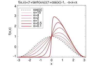
Figure 4: The density profile of the perturbations. A $\tanh$ function is used to introduce asymmetry. It has well behaved derivatives across the boundary and is suitable for periodic boundary conditions; see $\S 3.3$ for details.

3.3 Asymmetric Perturbation

The asymmetric perturbation is described by the following functional form.

$$f(\alpha,x)=\left(1+\tanh(x/\alpha)\right)(1+\cos{x})-1$$ (16)

The properties of this function are very similar to the $\cos$ function except that it is asymmetric. Some of the useful properties are as follows. It is defined in range $(-\pi,\pi)$ such that

$$f(\alpha,-\pi) = f(\alpha,\pi)=-1,$$ (17)

$$\frac{df(\alpha,x)}{dx}|_{x=-\pi} = \frac{df(\alpha,x)}{dx}|_{x=\pi}=0,$$ (18)

$$\langle f(\alpha,x)\rangle = \int_{-\pi}^{\pi}f(\alpha,x)dx=0$$ (19)

An asymmetric probability distribution for a periodic box of length $l$ with range $-l/2<x<l/2$, is given by

$$p(x)=\frac{l}{4\pi^{2}}\left(1+Af(\alpha,2\pi x/l)\right)$$

where $A$ is the amplitude of the perturbation. Note $p(x)>0$ only for $A\leq 1$. For $A>1$, this is the non-linear regime and then $p(x)$ can be negative. The amplitude of a cosine perturbation grows linearly with time. For simplicity, assuming the asymmetric perturbation to also behave in the same way, for our choice of ${\cal Z}_{\rm c}=2.0$ and ${\cal Z}_{\rm start}=6.36$, the amplitude $A$ from the growth factor is given by 0.3968.

4 Discussion

With apologies to John Donne, no galaxy is an island. Most galaxies are in groups and these accrete from the group environment which in turn accretes from the intergroup medium. This is a more accurate description for most galaxies than a simple statement of that galaxies accrete from the intergalactic medium. It is only in the last few years that modern simulations are able to show how this mechanism operates.

Our work was motivated by new large, ongoing surveys of galaxies (Bland-Hawthorn 2014; Bundy et al 2014) that seek to understand how the detailed properties of galaxies vary with the local environment. Motivated by the remarkable Bullet Cluster, we conjectured that asymmetries would lead to a large-scale separation of dark matter and baryons, thereby driving a dependence of galaxy properties with environment, but we do not find any evidence for this effect.

We do find, however, a mechanism for generating bulk flows in the galaxy population at a level that could explain the bulk flows of galaxies moving with respect to the cosmic microwave background. With our Gadget-2 simulation, we show that void asymmetries in the cosmic web can exacerbate local bulk flows of galaxies. The Cosmicflows-2 survey reveals that the Local Group resides in a “local sheet” of galaxies that borders a “local void” with a diameter of about 40 Mpc (Tully et al 2013). The void is found to be emptying out at a rate of 16 km s^-1 Mpc^-1. In a co-moving frame, the Local Sheet is found to be moving away from the Local Void at $\sim 260$ km s^-1. Our model shows how asymmetric collapse due to unbalanced voids on either side of a developing sheet or wall can lead to a systematic movement of the sheet, and the magnitude of the kinematic offset is (fortuitously) the same, at least in the early stages of the sheet collapse.

Our analysis seeks to honour the memory of Y.B. Zel’dovich whose published work continues to inspire astrophysicists around the world to the present day. We thank the organisers for putting together such an inspiring meeting.

JBH acknowledges an ARC Australian Laureate Fellowship and SS is funded by a University of Sydney DVC-R Fellowship. We are grateful to Merton College, Oxford for its hospitality in the final stages of writing up this work. We acknowledge insightful comments from T. Tepper-Garcia.

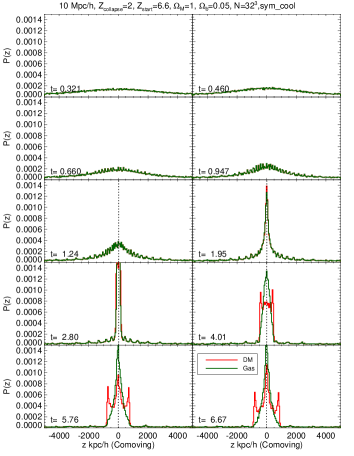
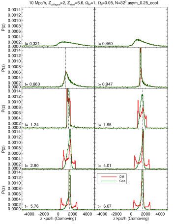
Figure 5: The $z$ distribution of particles as a function of time for a 10 Mpc h^-1, $N=32^{3}$ simulation. (Left) Symmetric case with cooling; (Right) Asymmetric perturbation $\alpha=0.25$ with cooling. The results for $\alpha\lesssim 1$ are very similar. The vertical lines show the location of the gas density peak. We do not mark the peak location at very early times, this is because it is difficult to locate the peak when the amplitude of the perturbation is very small.

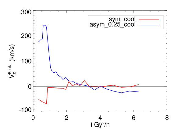
Figure 7: The evolution of the peculiar velocity of the peak (gas) for a 10 Mpc, $N=32^{3}$ simulation with periodic boundaries. For the case with the asymmetric perturbation the peak in density distribution is found to move with time. The peculiar velocity of peak is high at early times and then falls off with time.

References

- [Binney & Tremaine(2008)] Binney, J., & Tremaine, S. 2008, Galactic Dynamics: Second Edition, ISBN 978-0-691-13026-2, Princeton University Press, Princeton
- [Bland-Hawthorn(2014)] Bland-Hawthorn, J., in IAU Symp. 309, Galaxy in 3D across the Universe, B. L. Ziegler, F. Combes, H. Dannerbauer, M. Verdugo, Eds. (Cambridge: Cambridge Univ. Press), in press
- [Blanton & Moustakas(2009)] Blanton, M. R., & Moustakas, J. 2009, ARAA, 47, 159
- [Bundy et al.(2014)] Bundy K. et al. 2014, AJ, in press
- [Burstein et al.(1990)] Burstein, D., Faber, S. M., & Dressler, A. 1990, ApJ, 354, 18
- [Codis et al.(2012)] Codis, S., Pichon, C., Devriendt, J., et al. 2012, MNRAS, 427, 3320
- [Cooper et al.(2008)] Cooper, M. C., Tremonti, C. A., Newman, J. A., & Zabludoff, A. I. 2008, MNRAS, 390, 245
- [Croom S.(2012)] Croom, S.M., Lawrence, J.S., Bland-Hawthorn, J., Bryant, J.J. et al 2012, MNRAS, 421, 872
- [Dekel(1983)] Dekel, A. 1983, ApJ, 264, 373
- [Eldridge & Feix(1963)] Eldridge, O.C. & Feix, M. 1963, Phys. Fluids, 6, 398
- [Gómez et al.(2003)] Gómez, P. L., Nichol, R. C., Miller, C. J., et al. 2003, ApJ, 584, 210
- [Gordon & Lewis(2003)] Gordon, C., & Lewis, A. 2003, Phys. Rev. D, 67, 123513
- [Lewis et al.(2002)] Lewis, I., Balogh, M., De Propris, R., et al. 2002, MNRAS, 334, 673
- [Malaney & Mathews(1993)] Malaney, R. A., & Mathews, G. J. 1993, Phys. Rep., 229, 145
- [Mastropietro & Burkert(2008)] Mastropietro, C., & Burkert, A. 2008, MNRAS, 389, 967
- [Melott(1983)] Melott, A. L. 1983, MNRAS, 202, 595
- [Metuki et al.(2014)] Metuki, O., Libeskind, N.I., Hoffman, Y., Crain, R.A. & Theuns, T. 2014, astro-ph/1405.0281
- [Nichols & Bland-Hawthorn(2013)] Nichols, M., & Bland-Hawthorn, J. 2013, ApJ, 775, 97
- [Pichon et al.(2011)] Pichon, C., Pogosyan, D., Kimm, T. et al. 2011, MNRAS, 418, 2493
- [Rubin et al.(1976)] Rubin, V. C., Thonnard, N., Ford, W. K., Jr., & Roberts, M. S. 1976, AJ, 81, 719
- [Schaye et al.(2014)] Schaye, J., Crain, R. A., Bower, R. G., et al. 2014, arXiv:1407.7040
- [Shull et al.(2012)] Shull, J. M., Smith, B. D., & Danforth, C. W. 2012, ApJ, 759, 23
- [Sun et al.(2009)] Sun, M., Voit, G. M., Donahue, M., et al. 2009, ApJ, 693, 1142
- [Teles et al.(2011)] Teles, T. N., Levin, Y. & Pakter, R. 2011, MNRAS, 417, L21
- [Tully et al.(2008)] Tully, R. B., Shaya, E. J., Karachentsev, I. D., et al. 2008, ApJ, 676, 184
- [Tully et al.(2013)] Tully, R. B., Courtois, H. M., Dolphin, A. E., et al. 2013, AJ, 146, 86
- [Tumlinson et al.(2011)] Tumlinson, J., Thom, C., Werk, J. K., et al. 2011, Science, 334, 948
- [Vogelsberger et al.(2014)] Vogelsberger, M., Genel, S., Springel, V., et al. 2014, arXiv:1405.2921
- [Yamashiro et al.(1992)] Yamashiro, T., Gouda, N., & Sakagami, M. 1992, Progress of Theoretical Physics, 88, 269