Second-Order Asymptotic Optimality in
Multisensor Sequential Change Detection

Abstract

A generalized multisensor sequential change detection problem is considered, in which a number of (possibly correlated) sensors monitor an environment in real time, the joint distribution of their observations is determined by a global parameter vector, and at some unknown time there is a change in an unknown subset of components of this parameter vector. In this setup, we consider the problem of detecting the time of the change as soon as possible, while controlling the rate of false alarms. We establish the second-order asymptotic optimality (with respect to Lorden’s criterion) of various generalizations of the CUSUM rule; that is, we show that their additional expected worst-case detection delay (relative to the one that could be achieved if the affected subset was known) remains bounded as the rate of false alarm goes to 0, for any possible subset of affected components. This general framework incorporates the traditional multisensor setup in which only an unknown subset of sensors is affected by the change. The latter problem has a special structure which we exploit in order to obtain feasible representations of the proposed schemes. We present the results of a simulation study where we compare the proposed schemes with scalable detection rules that are only first-order asymptotically optimal. Finally, in the special case that the change affects exactly one sensor, we consider the scheme that runs in parallel the local CUSUM rules and study the problem of specifying the local thresholds.

1 Introduction

Suppose that a decision maker sequentially collects data from multiple streams, coming for example from sensors monitoring an environment. At some unknown point in time there is an abrupt change in the system that is perceived by either all or only a subset of the deployed sensors. The problem then is to combine the sequentially acquired observations from all streams in order to detect the change as quickly as possible, while controlling the rate of false alarms below an acceptable level. In what follows, we will refer to the various streams as “sensors”, although this general framework can be applied to various setups beyond environmental monitoring, such as intruder detection in computer security [1, 2, 3], epidemic detection in bio-surveillance [4, 5].

If the regime before and after the change is completely specified, one may apply a classical sequential change detection algorithm, such as the Cumulative Sum (CUSUM) rule, which was proposed by Page [6] and was shown by Moustakides [7] to be the best possible rule in Lorden’s [8] minimax setup in the case of iid observations before and after the change. However, in many applications that motivate this multisensor sequential change detection problem it is reasonable to assume that there is only partial information regarding the post-change regime. A typical assumption in the literature is that the change affects the distribution of only a subset of sensors whose identity is unknown. In this context, one needs to design detection rules that account for this uncertainty, and also to quantify how much is lost relative to the ideal case that the actual affected subset is known.

The simplest multisensor detection rule is the multichart CUSUM, according to which each sensor runs locally the CUSUM algorithm and the fusion center stops the first time an alarm is raised by any sensor. This is a one-shot scheme suitable for decentralized implementation, as each possibly remote sensor needs to communicate with the fusion center at most once, an important advantage in sensor networks that are characterized by limited bandwidth and energy. Tartakovksy et al. [1, 2] showed that this rule has a strong asymptotic optimality property when the change affects exactly one sensor (see also Section 9.2 in [9]). However, this rule is very inefficient when a large, or even a moderate, number of sensors are actually affected. This calls for detection rules that are robust, in the sense that they should perform well for a large class of scenarios regarding the subset of affected sensors.

In order to address this problem, Mei [10] proposed raising an alarm when the sum of the local CUSUM statistics exceeds a threshold, a rule to which we will refer as SUM-CUSUM. Under the assumptions of iid observations before/after the change, completely specified but arbitrary pre/post-change distributions (up to an integrability condition) and independent sensors it was shown that SUM-CUSUM is asymptotically optimal for every possible subset of affected sensors. Moreover, based on simulation experiments it was argued that SUM-CUSUM performs better than the multichart CUSUM unless a very small number of sensors is actually affected. This scheme was further refined by Mei in [11], where it was suggested to use the sum of only the top $L$ local CUSUM statistics when at most $L$ sensors can be affected. Liu et al. [12] and Banerjee and Veeravalli [13] considered further modifications that allow for only a subset of sensors to be employed at any given time.

A different, CUSUM-based, multisensor detection scheme was proposed by Xie and Siegmund [14]. Specifically, the proposed rule in this work was a modification of the CUSUM rule that corresponds to the case that the change occurs with probability $\pi$ in each sensor, where $\pi$ is the actual proportion of affected sensors. Asymptotic approximations for the operating characteristics of this detection rule were obtained in the case of independent sensors, each of which observes Gaussian iid observations whose mean may change from $0$ to some unknown value. Moreover, it was argued based on simulation experiments that this detection rule is more efficient than SUM-CUSUM and this phenomenon was explained on the basis that SUM-CUSUM does not incorporate the fact that all sensors are assumed to have the same change-point.

The main motivation for our work was to propose and study multisensor detection rules that enjoy a stronger asymptotic optimality property than SUM-CUSUM and are more efficient in practice. However, we consider a more general setup that incorporates applications that are not captured by the traditional multisensor framework, such as the power outage detection problem treated by Chen et al. [15]. Specifically, we assume that there is a global parameter vector that determines the joint distribution of the (possibly correlated) data streams and that the change modifies a subset of the components of this parameter vector. The affected subset of components is unknown, but it is assumed to belong to a given class of subsets, $\mathcal{P}$, that reflects our prior information regarding the location of the change. For example, in the extreme case that there is no information regarding the affected subset, $\mathcal{P}$ consists of all non-empty subsets of components.

In this generalized multisensor setup, we consider first of all the CUSUM-type rule that employs the Generalized Likelihood Ratio (GLR) statistic with respect to the unknown subset, to which we refer as GLR-CUSUM. Moreover, we consider two alternative, mixture-based CUSUM-type schemes. We show that all these detection rules enjoy a second-order asymptotic optimality property, i.e., that their additional worst-case detection delay (relative to the one that could be achieved if the affected subset was known) remains bounded as the rate of false alarms goes to 0 for any possible subset of affected components. This should be contrasted with the usual, weaker asymptotic optimality property, according to which the asymptotic relative efficiency goes to 1, and to which we refer as first-order asymptotic optimality.

Our general framework includes as a special case the traditional setup in which the change affects only an unknown subset of sensors, leaving the remaining ones completely unaffected. In this special case, assuming further independent sensors and an upper bound on the size of the affected subset, we obtain representations of the GLR-CUSUM (and one of the proposed mixture-based rule) which are feasible when the number of sensors is large. Moreover, we show that while the detection rule that was proposed by Xie and Siegmund [14] is also second-order asymptotically optimal for any choice of the parameter $\pi$, this parameter cannot be interpreted in this scheme as the proportion of affected sensors. Thus, we provide a theoretical explanation for the empirically observed superiority of this rule over SUM-CUSUM, which is only first-order asymptotically optimal, as well as its robustness with respect to $\pi$.

In the special case that it is known in advance that the change affects exactly one sensor, GLR-CUSUM reduces to the multichart CUSUM, according to which an alarm is raised when a local CUSUM statistic exceeds a local threshold. The selection of identical thresholds seems to be a default choice in the literature, although non-identical thresholds have also been considered (see, e.g. [9, p.467]). We address the problem of threshold selection in this setup and we show that seemingly reasonable threshold selections may lead to non-robust behavior, as the multichart CUSUM may fail to be even first-order asymptotically optimal. We then argue in favor of a specific selection of thresholds that equalizes the asymptotic relative performance loss under the various scenarios.

Let us discuss at this point the connection of our work with the literature of sequential change detection. Lorden [8] assumed (in a “single-sensor” setup) that the distribution of the observations belongs to an exponential family and is specified after the change up to an unknown parameter. In this context, he established the first-order asymptotic optimality of a CUSUM-type rule that is based on (a truncated away from 0 version of) the GLR statistic. In the special case of detecting a shift in the mean of Gaussian observations, Siegmund and Venkatraman [16] obtained approximations for the operating characteristics of the corresponding GLR-CUSUM. Our work differs from these two papers in that in our setup there is a finite number of scenarios in the post-change regime. Nevertheless, we also use the term GLR-CUSUM to describe the CUSUM-type rule whose detection statistic is based on maximizing with respect to the affected subset, which is the unknown parameter in our setup.

We should also mention an alternative formulation of the multisensor sequential change detection problem, in which the change-points in the various sensors are in generally different and the goal is to detect the first of them. This problem was considered from a Bayesian point of view by Ragavan and Veeravalli [17] and Ludkovski [18], where a model for the change propagation was assumed. A minimax approach was considered by Hadjiliadis et al. [19] and Zhang et al. [20], where it was shown that the multichart CUSUM has a strong asymptotic optimality property with respect to an extended Lorden criterion in which the worst case is taken with respect to all individual change-points and the history of observations up to the minimum of the change-points.

Another closely related problem to the one consider in this paper is the joint change detection and isolation problem, in which one is interested in isolating the affected subset upon detecting the change. While the GLR-CUSUM provides a natural estimator for this subset, a proper treatment of this problem requires a different formulation, in which the misclassification rate is also controlled together with the rate of false alarms. For more details on the joint sequential change detection and isolation problem we refer to Nikiforov [21, 22], Oskiper and Poor [23], Tartakovksy [24].

The rest of the paper is organized as follows: in Section 2 we formulate a general multisensor sequential change detection problem and establish the second-order asymptotic optimality of various CUSUM-based detection rules. In Section 3 we restrict ourselves to the traditional setup of independent sensors where only a subset of them is affected by the change. In Section 4 we focus on the case that the change affects exactly one sensor and the design of the multichart CUSUM. In Section 5 we present the findings of a simulation study that illustrates our asymptotic results. We conclude in Section 6, whereas we present the proofs of most results in Appendix. In what follows we set $x^{+}=\max\{x,0\}$, we use $|\cdot|$ to denote set cardinality, and we write $x\sim y$ when $x/y\rightarrow 1$, $x\simeq y$ when $x-y\rightarrow 0$.

2 A general multisensor sequential quickest detection problem

2.1 Problem formulation

Let $K$ be the number of sensors (streams) and $X_{t}^{k}$ the observation in sensor $k$ at time $t$, where $1\leq k\leq K$ and $t\in\mathbb{N}=\{1,2\ldots\}$. We assume that the random vectors $\{X_{t}\equiv(X_{t}^{1},\ldots,X_{t}^{K})\}_{t\in\mathbb{N}}$ are independent over time, but we allow observations from different sensors at the same time instant to be dependent. Moreover, we assume that the distribution of the sequence $\{X_{t}\}_{t\in\mathbb{N}}$ changes at some unknown deterministic time $\nu\in\mathbb{N}\cup\{0\}$. To be more specific, let $f(\cdot|\theta)$ be a family of densities with respect to some dominating $\sigma$-finite measure, where $\theta$ is a $N$-dimensional parameter vector and $N$ not necessarily equal to $K$. Then, we assume that $X_{t}\sim f(\cdot|\theta_{t})$, where $\theta_{t}:=(\theta_{t}^{1},\ldots,\theta_{t}^{N})$ is given by

$$\begin{split}\theta_{t}^{k}&=0\quad\forall\;1\leq k\leq N,\quad t\leq\nu,\\ \theta_{t}^{k}&=\begin{cases}1,&\quad k\in\mathcal{A},\\ 0,&\quad k\notin\mathcal{A},\end{cases}\qquad t>\nu,\end{split}$$ (1)

and $\mathcal{A}\subset\{1,\ldots,N\}$ is a subset of components of $\theta_{t}$. Note that the change may affect the observations in all sensors and that while the pre-change distribution is completely specified, the post-change distribution is specified up to subset $\mathcal{A}$ which is typically unknown. However, we will assume that the true affected subset belongs to a given class $\mathcal{P}$ of subsets of $\{1,\ldots,N\}$. For example, if it is known that the change will affect exactly (resp. at most) $L$ components of $\theta$, then $\mathcal{P}=\mathcal{P}_{L}$ (resp. $\mathcal{P}=\overline{\mathcal{P}}_{L}$), where

$$\begin{split}\mathcal{P}_{L}&:=\{\mathcal{A}:|\mathcal{A}|=L\},\\ \overline{\mathcal{P}}_{L}&:=\{\mathcal{A}:1\leq|\mathcal{A}|\leq L\},\end{split}$$ (2)

$|\mathcal{A}|$ being the cardinality of subset $\mathcal{A}$ and $1\leq L\leq N$. Note that $\overline{\mathcal{P}}_{N}$ corresponds to the case of complete ignorance regarding the affected subset. Moreover, any class $\mathcal{P}$ is a subset of a class of the form $\overline{\mathcal{P}}_{L}$ for some $1\leq L\leq N$. However, in what follows we do not make any assumption about $\mathcal{P}$ unless this is explicitly stated.

Let ${\sf P}_{\infty}$ and $\operatorname{{\sf E}}_{\infty}$ the probability measure and the expectation when the change never occurs ($\nu=\infty$) and ${\sf P}^{\mathcal{A}}_{\nu}$ and $\operatorname{{\sf E}}^{\mathcal{A}}_{\nu}$ the probability measure and the expectation when the change occurs at time $\nu$ only in subset $\mathcal{A}$. A sequential change detection rule is an $\{{\mathcal{F}}_{t}\}$-stopping time, $T$, at which the fusion center raises an alarm declaring that the change has occurred. Here, ${\mathcal{F}}_{t}$ the $\sigma$-algebra generated by all observations up to time $t$, i.e., ${\mathcal{F}}_{t}:=\sigma(X_{s};\;1\leq s\leq t)$. Following Lorden’s approach [8] we measure the performance of a detection rule $T$ when the change occurs in subset $\mathcal{A}$ with the worst (with respect to the change point) conditional expected delay given the worst possible history of observations up to the change point:

$$\mathcal{J}_{\mathcal{A}}[T]:=\sup_{\nu\geq 0}\operatorname*{ess\,sup}\operatorname{{\sf E}}^{\mathcal{A}}_{\nu}[(T-\nu)^{+}\,|\,\mathcal{F}_{\nu}].$$

Moreover, we control the rate of false alarms below an acceptable, user-specified level $\gamma\geq 1$, thus, we restrict ourselves to sequential detection rules in the class $\mathcal{C}_{\gamma}=\{T:\,\operatorname{{\sf E}}_{\infty}[T]\geq\gamma\}$. We will be interested in sequential detection rules that attain the optimal performance $\inf_{T\in\mathcal{C}_{\gamma}}\mathcal{J}_{\mathcal{A}}[T]$ for every $\mathcal{A}\in\mathcal{P}$ asymptotically as $\gamma\rightarrow\infty$.

Definition 1.

Suppose that the detection rule $T^{*}$ can be designed so that $T^{*}\in\mathcal{C}_{\gamma}$ for any given $\gamma\geq 1$. We will say that $T^{*}$ is asymptotically optimal of

1. first-order, if for every $\mathcal{A}\in\mathcal{P}$ we have as $\gamma\rightarrow\infty$

   $$\mathcal{J}_{\mathcal{A}}[T^{*}]\sim\inf_{T\in\mathcal{C}_{\gamma}}\mathcal{J}_{\mathcal{A}}[T],$$

2. second-order, if for every $\mathcal{A}\in\mathcal{P}$ we have

   $$\mathcal{J}_{\mathcal{A}}[T^{*}]-\inf_{T\in\mathcal{C}_{\gamma}}\mathcal{J}_{\mathcal{A}}[T]={\mathcal{O}}(1),$$

   where ${\mathcal{O}}(1)$ is a bounded term as $\gamma\rightarrow\infty$.

Remark: If $T^{*}$ is first-order asymptotically optimal, then it is possible that for some $\mathcal{A}\in\mathcal{P}$ we have $\mathcal{J}_{\mathcal{A}}[T^{*}]-\inf_{T\in\mathcal{C}_{\gamma}}\mathcal{J}_{\mathcal{A}}[T]\rightarrow\infty,$ since both terms go to infinity as $\gamma\rightarrow\infty$. In such a case, the additional (worst-case) expected number of observations that $T^{*}$ requires (relative to the corresponding optimal detection delay that would be achievable if the actual affected subset was known) is unbounded as the rate of false alarms goes to $0$. This motivates the stronger notion of second-order asymptotic optimality.

It is the main goal of this work to propose detection rules that are second-order asymptotically optimal. In order to do so, we need to characterize the optimal performance that is attained by the oracle detection rule.

2.2 The oracle rule

For any given subset $\mathcal{A}$, the solution to the constrained optimization problem $\inf_{T\in\mathcal{C}_{\gamma}}\mathcal{J}_{\mathcal{A}}[T]$ is well known. In order to describe it, let us set

$$\Lambda_{t}^{\mathcal{A}} :=\frac{d{\sf P}_{0}^{\mathcal{A}}}{d{\sf P}_{\infty}}({\mathcal{F}}_{t})\quad\text{and}\quad Z_{t}^{\mathcal{A}}:=\log\Lambda_{t}^{\mathcal{A}}$$ (3)

and note that due to the assumption of independence over time we have

$$\Lambda_{t}^{\mathcal{A}} =\Lambda_{t-1}^{\mathcal{A}}\cdot\exp\{\ell_{t}^{\mathcal{A}}\},\quad\Lambda_{0}^{\mathcal{A}}:=1,$$

$$Z_{t}^{\mathcal{A}} =Z_{t-1}^{\mathcal{A}}+\ell_{t}^{\mathcal{A}},\quad Z_{0}^{\mathcal{A}}:=0,$$

where $\ell_{t}^{\mathcal{A}}$ is the log-likelihood ratio

$$\ell_{t}^{\mathcal{A}} :=\log\frac{d{\sf P}_{0}^{\mathcal{A}}}{d{\sf P}_{\infty}}(X_{t}).$$ (4)

The CUSUM rule for detecting a change in subset $\mathcal{A}$ is

$$S^{\mathcal{A}}_{b} =\inf\left\{t\in\mathbb{N}:\tilde{Y}^{\mathcal{A}}_{t}\geq b\right\},$$ (5)

where $b\in\mathbb{R}$ is a deterministic threshold and $\tilde{Y}^{\mathcal{A}}$ is the so-called CUSUM statistic

$$\tilde{Y}^{\mathcal{A}}_{t}:=Z_{t}^{\mathcal{A}}-\min_{0\leq s<t}Z_{s}^{\mathcal{A}},\quad t\in\mathbb{N},$$ (6)

which may be equivalently defined through the following recursion

$$\tilde{Y}^{\mathcal{A}}_{t}=\max\{\tilde{Y}_{t-1}^{\mathcal{A}}\,,\,0\}+\ell_{t}^{\mathcal{A}},\quad\tilde{Y}_{0}^{\mathcal{A}}:=0.$$ (7)

Moustakides [7] showed that, for any given $\gamma\geq 1$, $S_{b}^{\mathcal{A}}$ optimizes Lorden’s criterion, $\mathcal{J}_{\mathcal{A}}$, in the class $\mathcal{C}_{\gamma}$, when threshold $b$ is chosen so that $\operatorname{{\sf E}}_{\infty}[S^{\mathcal{A}}_{b}]=\gamma$. Earlier, Lorden [8] had established the first-order asymptotic optimality of the CUSUM rule by showing that

$$\inf_{T\in\mathcal{C}_{\gamma}}\mathcal{J}_{\mathcal{A}}[T] \sim\frac{\log\gamma}{I_{\mathcal{A}}},\quad I_{\mathcal{A}}:=\operatorname{{\sf E}}_{0}^{\mathcal{A}}[\ell_{1}^{\mathcal{A}}],$$ (8)

under the assumption that $\ell_{1}^{\mathcal{A}}$ is ${\sf P}_{0}^{\mathcal{A}},{\sf P}_{\infty}$- integrable. However, the exact optimality of the CUSUM rule can be used to obtain a second-order characterization of the optimal performance. Indeed, if additionally we have $\operatorname{{\sf E}}_{0}^{\mathcal{A}}[(\ell_{1}^{\mathcal{A}})^{2}]<\infty$, it is well known (see, e.g., [9], [25]) that

$$\operatorname{{\sf E}}_{0}^{\mathcal{A}}[S_{b}^{\mathcal{A}}]=\frac{b}{I_{\mathcal{A}}}+\Theta(1),$$

where $\Theta(1)$ is a term that is bounded from above and below as $b\rightarrow\infty$. Moreover, from [26] it follows that $\operatorname{{\sf E}}_{\infty}[S_{b}^{\mathcal{A}}]\sim e^{b}/v_{\mathcal{A}}$ as $b\rightarrow\infty$, where $v_{\mathcal{A}}$ is a model-dependent, renewal-theoretic constant. Therefore, we conclude that

$$\inf_{T\in\mathcal{C}_{\gamma}}\mathcal{J}_{\mathcal{A}}[T]=\frac{\log\gamma}{I_{\mathcal{A}}}+\Theta(1).$$

We summarize these characterizations of first and second order asymptotic optimality in the following Lemma.

Lemma 1.

1. Suppose that $\ell_{1}^{\mathcal{A}}$ is integrable with respect to ${\sf P}_{\infty}$ and ${\sf P}_{0}^{\mathcal{A}}$ for every $\mathcal{A}\in\mathcal{P}$ and that, for any given $\gamma\geq 1$, a detection rule $T^{*}$ can be designed so that $T^{*}\in\mathcal{C}_{\gamma}$. If

   $$\mathcal{J}_{\mathcal{A}}[T^{*}]\leq\frac{\log\gamma}{I_{\mathcal{A}}}(1+o(1)),\quad\;\forall\;\mathcal{A}\in\mathcal{P},$$

   then $T^{*}$ is first-order asymptotically optimal with respect to class $\mathcal{P}$.

2. Suppose additionally that $\ell_{1}^{\mathcal{A}}$ is square-integrable with respect to ${\sf P}_{0}^{\mathcal{A}}$ for every $\mathcal{A}\in\mathcal{P}$. If

   $$\mathcal{J}_{\mathcal{A}}[T^{*}]\leq\frac{\log\gamma}{I_{\mathcal{A}}}+{\mathcal{O}}(1),\quad\;\forall\;\mathcal{A}\in\mathcal{P},$$

   then $T^{*}$ is second-order asymptotically optimal with respect to class $\mathcal{P}$.

Remark: It is useful to stress that the CUSUM statistic is often defined in the literature as

$$Y^{\mathcal{A}}_{t}:=Z_{t}^{\mathcal{A}}-\min_{0\leq s\leq t}Z_{s}^{\mathcal{A}},$$ (9)

or equivalently through the following recursion

$$Y^{\mathcal{A}}_{t}=\max\left\{Y_{t-1}^{\mathcal{A}}+\ell_{t}^{\mathcal{A}}\,,\,0\right\},\quad Y_{0}^{\mathcal{A}}:=0.$$

Thus, $Y^{\mathcal{A}}_{t}$ differs from $\tilde{Y}^{\mathcal{A}}_{t}$ only when the latter is negative, and the two statistics lead to the same stopping time when the threshold $b$ is positive. However, with the non-negative version of the CUSUM statistic it is not in general possible to satisfy the false alarm constraint for any $\gamma>1$. Since in this work we focus on asymptotic optimality results, we will use both versions of the CUSUM statistic, depending on which one is more technically convenient each time.

2.3 Generalized and Mixture based CUSUM rules

We now construct various multichannel detection rules that will be shown to be second-order asymptotically optimal with respect to any given class $\mathcal{P}$. In order to do so, suppose for the moment that the affected subset is $\mathcal{A}\in\mathcal{P}$. At some time $t>\nu$, the likelihood ratio of ${\sf P}_{\nu}^{\mathcal{A}}$ versus ${\sf P}_{\infty}$ is given by

$$\frac{\Lambda_{t}^{\mathcal{A}}}{\Lambda_{\nu}^{\mathcal{A}}}=\frac{d{\sf P}_{\nu}^{\mathcal{A}}}{d{\sf P}_{\infty}}({\mathcal{F}}_{t})=\prod_{s=\nu+1}^{t}\exp(\ell_{s}^{\mathcal{A}}),$$

and the corresponding log-likelihood ratio takes the form

$$Z_{t}^{\mathcal{A}}-Z_{\nu}^{\mathcal{A}}=\log\frac{\Lambda_{t}^{\mathcal{A}}}{\Lambda_{\nu}^{\mathcal{A}}}=\sum_{s=\nu+1}^{t}\ell_{s}^{\mathcal{A}},$$

where $\Lambda_{t}^{\mathcal{A}}$, $Z_{t}^{\mathcal{A}}$ and $\ell_{t}^{\mathcal{A}}$ are defined in (3) and (4), respectively. Maximizing with respect to both the unknown change-point, $\nu$, and the unknown subset, $\mathcal{A}$, suggests raising an alarm when the statistic

$$\max_{0\leq s<t}\max_{\mathcal{A}\in\mathcal{P}}(Z_{t}^{\mathcal{A}}-Z_{s}^{\mathcal{A}})$$

becomes larger than some threshold $b$. Interchanging the two maximizations reveals that this detection statistic can be equivalently expressed as

$$\max_{\mathcal{A}\in\mathcal{P}}\max_{0\leq s<t}(Z_{t}^{\mathcal{A}}-Z_{s}^{\mathcal{A}})=\max_{\mathcal{A}\in\mathcal{P}}\tilde{Y}_{t}^{\mathcal{A}},$$

where $\tilde{Y}^{\mathcal{A}}$ is defined in (6). Therefore, this rule stops the first time $t$ there is a subset $\mathcal{A}$ whose corresponding CUSUM statistic $\tilde{Y}_{t}^{\mathcal{A}}$ exceeds threshold $b$. If we only consider positive thresholds, we may equivalently consider the detection statistic $\max_{\mathcal{A}\in\mathcal{P}}Y_{t}^{\mathcal{A}}$, where $Y^{\mathcal{A}}$ is defined in (9) (see the remark in the end of the previous subsection).

We can generalize this scheme by allowing the thresholds that correspond to the various CUSUM statistics to differ. Thus, if $\{b_{\mathcal{A}},\mathcal{A}\in\mathcal{P}\}$ is a family of positive, constant thresholds, we obtain the following detection rule, to which we refer as GLR-CUSUM:

$$\min_{\mathcal{A}\in\mathcal{P}}S^{\mathcal{A}}_{b_{\mathcal{A}}} =\inf\left\{t\in\mathbb{N}:\max_{\mathcal{A}\in\mathcal{P}}\,(Y_{t}^{\mathcal{A}}-b_{\mathcal{A}})\geq 0\right\},$$ (10)

(Recall that $S^{\mathcal{A}}_{b}$ is the CUSUM rule defined in (5)). We will show in Proposition 3 that some intuitively reasonable threshold specifications, such as selecting each threshold $b_{\mathcal{A}}$ proportionally to the Kullback-Leibler divergence $I_{\mathcal{A}}$, may fail to guarantee even the first-order asymptotic optimality of GLR-CUSUM. For this reason, in what follows we restrict our attention to thresholds of the form

$$b_{\mathcal{A}}=b-\log p_{\mathcal{A}},$$

where $b$ is a positive threshold that is determined by the false alarm constraint and depends on $\gamma$, whereas $\{p_{\mathcal{A}},\mathcal{A}\in\mathcal{P}\}$ are constants (weights) that do not depend on $\gamma$ and satisfy

$$p_{\mathcal{A}}>0\quad\!\forall\;\mathcal{A}\in\mathcal{P}\quad\text{and}\quad\sum_{\mathcal{A}\in\mathcal{P}}p_{\mathcal{A}}=1.$$

With this threshold specification the GLR-CUSUM in (10) takes the form

$$S_{b} :=\inf\left\{t\in\mathbb{N}:\max_{\mathcal{A}\in\mathcal{P}}\left(Y_{t}^{\mathcal{A}}+\log p_{\mathcal{A}}\right)\geq b\right\}$$ (11)

and may be equivalently expressed as follows

$$S_{b} =\inf\left\{t\in\mathbb{N}:\max_{0\leq s\leq t}\max_{\mathcal{A}\in\mathcal{P}}\left(Z_{t}^{\mathcal{A}}-Z_{s}^{\mathcal{A}}+\log p_{\mathcal{A}}\right)\geq b\right\}$$

$$=\inf\left\{t\in\mathbb{N}:\max_{0\leq s\leq t}\max_{\mathcal{A}\in\mathcal{P}}p_{\mathcal{A}}\exp(Z_{t}^{\mathcal{A}}-Z_{s}^{\mathcal{A}})\geq e^{b}\right\}.$$ (12)

When the $p_{\mathcal{A}}$’s are identical, we will refer to $S_{b}$ as the unweighted GLR-CUSUM. However, the introduction of weights allows us to present the GLR-CUSUM together with competitive mixture-based CUSUM tests. Specifically, if we do not maximize but average with respect to the affected subset in (12), we obtain the following stopping time:

$$\bar{S}_{b} :=\inf\left\{t\in\mathbb{N}:\max_{0\leq s\leq t}\sum_{\mathcal{A}\in\mathcal{P}}p_{\mathcal{A}}\exp(Z_{t}^{\mathcal{A}}-Z_{s}^{\mathcal{A}})\geq e^{b}\right\}.$$ (13)

If we further interchange maximization and summation in the detection statistic in (13), we obtain the alternative detection statistic $\sum_{\mathcal{A}\in\mathcal{P}}p_{\mathcal{A}}\exp(Y_{t}^{\mathcal{A}}).$ For technical convenience, we replace $Y^{\mathcal{A}}$ with $\tilde{Y}^{\mathcal{A}}$ and set

$$\tilde{S}_{b}:=\inf\left\{t\in\mathbb{N}:\sum_{\mathcal{A}\in\mathcal{P}}p_{\mathcal{A}}\,\exp(\tilde{Y}_{t}^{\mathcal{A}})\geq e^{b}\right\}.$$ (14)

To sum up, we have introduced three distinct multichannel detection rules: the GLR-CUSUM, $S_{b}$, which can be equivalently defined by either (11) or (12), and two mixture-based CUSUM rules, $\bar{S}_{b}$ and $\tilde{S}_{b}$, defined in (13) and (14) respectively. In the following theorem, whose proof can be found in the Appendix, we establish their second-order asymptotic optimality property with respect to an arbitrary class $\mathcal{P}$.

Theorem 1.

For an arbitrary class $\mathcal{P}$,

1. if $b=\log\gamma$, then $S_{b},\bar{S}_{b},\tilde{S}_{b}\in\mathcal{C}_{\gamma}$;

2. if $\ell_{1}^{\mathcal{A}}$ is square-integrable with respect to ${\sf P}_{0}^{\mathcal{A}}$ for every $\mathcal{A}\in\mathcal{P}$, then $S,\bar{S},\tilde{S}$ are second-order asymptotically optimal with respect to $\mathcal{P}$.

Although it was not needed in the proof of the previous theorem, it is important (and useful for computational purposes) to note that the worst-case scenario for all the above detection rules is when $\nu=0$. This is the content of the following proposition, whose proof can be found in the Appendix.

Proposition 1.

For any $b>0$ and $\mathcal{A}\in\mathcal{P}$ we have

$$i)\;\mathcal{J}_{\mathcal{A}}[S_{b}]=\operatorname{{\sf E}}_{0}^{\mathcal{A}}[S_{b}],\quad ii)\;\mathcal{J}_{\mathcal{A}}[\bar{S}_{b}]=\operatorname{{\sf E}}_{0}^{\mathcal{A}}[\bar{S}_{b}],\quad iii)\;\mathcal{J}_{\mathcal{A}}[\tilde{S}_{b}]=\operatorname{{\sf E}}_{0}^{\mathcal{A}}[\tilde{S}_{b}].$$

2.4 Implementation

The two representations of the GLR-CUSUM, (11) and (12), suggest two possible approaches regarding its implementation. According to the first one, at each time $t$ we compute and maximize over the CUSUM statistics, $Y_{t}^{\mathcal{A}}$, $\mathcal{A}\in\mathcal{P}$. This approach requires running $|\mathcal{P}|$ recursions and is convenient when the cardinality of $\mathcal{P}$ is small. This is for example the case when only one component of the parameter vector $\theta$ is affected by the change ($\mathcal{P}=\mathcal{P}_{1}$), in which case $|\mathcal{P}|=N$. However, such an implementation may not be feasible for large values of $N$ when we have complete ignorance regarding the affected subset ($\mathcal{P}=\overline{\mathcal{P}}_{N}$). (This approach also applies to the mixture-based CUSUM rule defined in (14), which sums over the exponents of all CUSUM statistics).

According to the second approach, at each time $t$ we need to compute and maximizer over the statistics $Z_{t}^{\mathcal{A}}-Z_{s}^{\mathcal{A}}+\log p_{\mathcal{A}}$, $0\leq s<t$, $\mathcal{A}\in\mathcal{P}$. In the next section we will see that this computation is simplified in the special case that we have independent sensors and only a subset of which is affected by the change. Moreover, in the next lemma we show that, without any loss, we can always restrict the maximization to an adaptive time-window. Since a similar approach applies to the mixture-based CUSUM defined in (13), we state the following lemma in some generality.

Lemma 2.

Let $\mathcal{P}$ be an arbitrary class and consider the following sequence of stopping times

$$\begin{split}r_{n+1}&=\inf\left\{{t>r_{n}}\,:\,{Z_{t}^{\mathcal{A}}=\min_{0\leq s\leq t}Z_{s}^{\mathcal{A}},\quad\text{for all $\mathcal{A}\in\mathcal{P}$}}\right\};\;r_{0}=0.\end{split}$$ (15)

Then for any function $G:\mathbb{R}^{|\mathcal{P}|}\to\mathbb{R}$ that is non-decreasing in each of its arguments,

$$\inf\left\{{t\geq 0}\,:\,{\max_{0\leq s\leq t}G\left((Z_{t}^{\mathcal{A}}-Z_{s}^{\mathcal{A}})_{\mathcal{A}\in\mathcal{P}}\right)\geq b}\right\}$$

$$=\inf\left\{{t\geq 0}\,:\,{\max_{r(t)\leq s\leq t}G\left((Z_{t}^{\mathcal{A}}-Z_{s}^{\mathcal{A}})_{\mathcal{A}\in\mathcal{P}}\right)\geq b}\right\}$$ ,

where $(\cdot)_{\mathcal{A}\in\mathcal{P}}$ denotes a $\mathcal{P}$-tuple and $r(t)=\max\left\{{r_{n}}\,:\,{r_{n}\leq t}\right\}$.

Proof.

Fix $t>0$. Since $G$ is non-decreasing in each of its arguments, it suffices to show that for every $0\leq s\leq r(t)$ and $\mathcal{A}\in\mathcal{P}$ we have $Z_{t}^{\mathcal{A}}-Z_{s}^{\mathcal{A}}\leq Z_{t}^{\mathcal{A}}-Z_{r(t)}^{\mathcal{A}}$, or equivalently $Z_{r(t)}^{\mathcal{A}}\leq Z_{s}^{\mathcal{A}}$, which follows from the definition of $r(t)$. ∎

3 A special multisensor sequential change-detection problem

3.1 A special case of the general framework

In this section, we focus on the special case that the change affects the distribution of only a subset of sensors. In order to be more specific, let us recall that at each time $t$ we observe a random vector $X_{t}=(X_{t}^{1},\ldots,X_{t}^{K})$ with joint density $X_{t}\sim f(\cdot|\theta_{t})$, where $\theta_{t}=(\theta_{t}^{1},\ldots,\theta_{t}^{N})$ is an unobserved parameter vector. Let $f_{k}$ be the marginal density of the $k^{\text{th}}$ stream, i.e., $X_{t}^{k}\sim f_{k}(\cdot|\theta_{t})$. In what follows, we assume that the dimensions of $X_{t}$ and $\theta_{t}$ coincide, i.e., $N=K$, and that each marginal density $f_{k}(\cdot|\theta_{t})$ is determined only by the $k^{\text{th}}$ component of $\theta_{t}$, $\theta_{t}^{k}$. Specifically, we assume that

$$f_{k}(\cdot|\theta_{t}^{k}=0) =h_{k},\quad f_{k}(\cdot|\theta_{t}^{k}=1)=g_{k},$$

where $h_{k}$ and $g_{k}$ are completely specified densities with respect to some $\sigma$-finite measure $\lambda_{k}$. Note that $h_{k}$ and $g_{k}$ do not need to belong in the same parametric family, our only assumption is that their Kullback-Leibler information number,

$$I_{k}:=\int\log\left(\frac{g_{k}}{h_{k}}\right)\;g_{k}\;d\lambda_{k},$$ (16)

is positive and finite. Therefore, in this setup we have a change in the marginal distributions of a subset of sensors, while the remaining ones remain completely unaffected, and the change detection problem (1) takes the form

$$\begin{split}X_{t}^{k}&\sim h_{k},\quad\forall\;1\leq k\leq K,\quad t\leq\nu,\\ X_{t}^{k}&\sim\begin{cases}g_{k},&\quad k\in\mathcal{A},\\ h_{k},&\quad k\notin\mathcal{A},\end{cases}\quad t>\nu,\end{split}$$ (17)

where $\mathcal{A}\subset\{1,\ldots,K\}$ is a subset of sensors that belongs to some class $\mathcal{P}$. When in particular $\mathcal{P}=\mathcal{P}_{L}$ (resp. $\mathcal{P}=\overline{\mathcal{P}}_{L}$), the change affects exactly (resp. at most) $L$ sensors, where the classes $\mathcal{P}_{L}$ and $\overline{\mathcal{P}}_{L}$ are defined in (2).

In the literature of the multisensor quickest detection problem it is typically assumed that observations from different streams are independent. However, this is not necessary for the results of the previous section to hold. This is illustrated by the following example.

Example: Correlated normal streams

Let $\Sigma$ be an invertible covariance matrix of dimension $K$ with diagonal $(\sigma_{1}^{2},\ldots,\sigma_{K}^{2})$ and let $\mu_{1},\ldots,\mu_{K}$ be non-zero constants. For every non-empty subset $\mathcal{A}\subset\{1,\ldots,K\}$ we define the $K$-dimensional vector $\mu_{\mathcal{A}}:=(\mu_{1}^{\mathcal{A}},\ldots,\mu_{K}^{\mathcal{A}})$ such that

$$\mu_{k}^{\mathcal{A}}:=\begin{dcases}\mu_{k},&\;k\in\mathcal{A},\\ 0,&\;k\notin\mathcal{A},\end{dcases}$$

and we assume that under ${\sf P}_{\nu}^{\mathcal{A}}$ we have

$$X_{t}\sim\begin{dcases}\mathcal{N}(0,\Sigma),&t\leq\nu,\\ \mathcal{N}(\mu_{\mathcal{A}},\Sigma),&t>\nu.\end{dcases}$$

Then, this is a special case of (17) with $h_{k}=\mathcal{N}(0,\sigma_{k}^{2})$ and $g_{k}=\mathcal{N}(\mu_{k},\sigma_{k}^{2})$, for which

$$\ell_{t}^{\mathcal{A}}=\theta_{\mathcal{A}}\cdot X_{t}-\frac{1}{2}\theta_{\mathcal{A}}\cdot\mu_{\mathcal{A}},\quad\quad\theta_{\mathcal{A}}:=\Sigma^{-1}\mu_{\mathcal{A}},$$

where $\ell_{t}^{\mathcal{A}}$ is the log-likelihood ratio defined in (4).

3.2 The case of independent sensors

We now restrict ourselves to the case of independent sensors. Specifically, we assume that the local filtrations $\{\mathcal{F}_{t}^{1}\},\ldots,\{\mathcal{F}_{t}^{K}\}$ are independent, where ${\mathcal{F}}_{t}^{k}:=\sigma(X_{s}^{k},\;1\leq s\leq t)$, $1\leq k\leq K$. Under this assumption, the log-likelihood ratio statistic $\ell_{t}^{\mathcal{A}}$, defined in (4), admits the following decomposition

$$\ell_{t}^{\mathcal{A}}=\sum_{k\in\mathcal{A}}\ell_{t}^{k},\quad\quad\ell_{t}^{k}:=\log\frac{g_{k}}{h_{k}}(X_{t}^{k}),$$ (18)

which implies that the likelihood and log-likelihood ratio statistics, $\Lambda_{t}^{\mathcal{A}}$ and $Z_{t}^{\mathcal{A}}$, defined in (3), take the form

$$\Lambda_{t}^{\mathcal{A}} =\prod_{k\in\mathcal{A}}\Lambda_{t}^{k},\quad\Lambda_{t}^{k}:=\Lambda_{t-1}^{k}\,\exp\{\ell_{t}^{k}\},\quad\Lambda_{0}^{k}=1,$$

$$Z_{t}^{\mathcal{A}} =\sum_{k\in\mathcal{A}}Z_{t}^{k},\quad Z_{t}^{k}:=Z_{t-1}^{k}+\ell_{t}^{k},\quad Z_{0}^{k}=0.$$

Moreover, we have $I_{\mathcal{A}}=\sum_{k\in\mathcal{A}}I_{k}$, where $I_{\mathcal{A}}$ is the Kullback-Leibler information number defined in (8) and $I_{k}$ the local Kullback-Leibler information number defined in (16). If we further select weights of the form

$$p_{\mathcal{A}} =\frac{p^{|\mathcal{A}|}}{\sum_{\mathcal{B}\in\mathcal{P}}p^{|\mathcal{B}|}},$$ (19)

where $p$ is some arbitrary positive parameter, then from (12) and (13) it follows that the GLR-CUSUM and the mixture-based CUSUM rule, $\bar{S}_{b}$, can be expressed as follows:

$$S_{b} :=\inf\left\{t\in\mathbb{N}:\max_{0\leq s\leq t}\,\max_{\mathcal{A}\in\mathcal{P}}\sum_{k\in\mathcal{A}}\left(Z_{t}^{k}-Z_{s}^{k}+\log p\right)\geq b+\log(C(\mathcal{P}))\right\},$$ (20)

$$\bar{S}_{b} :=\inf\left\{t\in\mathbb{N}:\max_{0\leq s\leq t}\sum_{\mathcal{A}\in\mathcal{P}}p^{|\mathcal{A}|}\prod_{k\in\mathcal{A}}\exp(Z_{t}^{k}-Z_{s}^{k})\geq e^{b}\,C(\mathcal{P})\right\},$$ (21)

where $C(\mathcal{P}):=\sum_{\mathcal{B}\in\mathcal{P}}p^{|\mathcal{B}|}$. In the following proposition, whose proof is presented in the Appendix, we show that the latter expressions can be further simplified for classes of the form $\mathcal{P}_{L}$ and $\overline{\mathcal{P}}_{L}$. In order to do so, for any $0\leq s\leq t$ we set

$$Z_{s:t}^{k}:=Z_{t}^{k}-Z_{s}^{k},\quad 1\leq k\leq K,$$

and we introduce the corresponding order statistics $Z_{s:t}^{(1)}\geq\ldots\geq Z_{s:t}^{(K)}.$

Proposition 2.

Consider the change detection problem (17) and suppose that the independence assumption (18) holds.

(i) The GLR-CUSUM in (20) takes the form

$$\inf\Bigl{\{}t\in\mathbb{N}:\max_{0\leq s\leq t}\sum_{k=1}^{L}Z_{s:t}^{(k)}\geq b+\log|\mathcal{P}_{L}|\Bigr{\}}\quad\text{when}\quad\mathcal{P}=\mathcal{P}_{L},$$ (22)

$$\inf\left\{t\in\mathbb{N}:\max_{0\leq s\leq t}\sum_{k=1}^{L}\left(Z_{s:t}^{(k)}+\log p\right)^{+}\geq b+\log\left(\sum_{k=1}^{L}|\mathcal{P}_{k}|\,p^{k}\right)\right\}\quad\text{when}\quad\mathcal{P}=\overline{\mathcal{P}}_{L}.$$ (23)

(ii) When $\mathcal{P}=\overline{\mathcal{P}}_{K}$, the mixture rule $\bar{S}_{b}$ in (21) takes the form

$$\hat{S}_{\hat{b}}(\pi) :=\inf\left\{t\in\mathbb{N}:\max_{0\leq s\leq t}\prod_{k=1}^{K}\left[1-\pi+\pi\,\exp(Z_{t}^{k}-Z_{s}^{k})\right]\geq\exp\{\hat{b}\}\right\},$$ (24)

where $\pi=p/(1+p)$ and

$$\exp\{\hat{{b}}\}:=(1-\pi)^{-K}\left(\exp\{b\}\sum_{\mathcal{B}\in\mathcal{P}}p^{|\mathcal{B}|}+1\right).$$

Remark: From Lemma 2 we know that we can replace $\max_{0\leq s\leq t}$ in the above detection rules by $\max_{r(t)\leq s\leq t}$, where $r(t)=\max\{n:r_{n}\leq t\}$ and the sequence of stopping times $(r_{n})$ are defined in (15). In the case of independent sensors that consider in this section we have $Y_{t}^{\mathcal{A}}\leq\sum_{k\in\mathcal{A}}Y_{t}^{k}$ for every $t$ and $\mathcal{A}$, which implies that for a class of the form $\overline{\mathcal{P}}_{L}$ the times $(r_{n})$ can be defined as follows:

$$r_{n} =\inf\left\{{t>r_{n-1}}\,:\,{Z_{t}^{k}=\min_{0\leq s\leq t}Z_{s}^{k},\quad\forall\,1\leq k\leq K}\right\},$$

where $r_{0}:=0$. From Proposition 1 in [10] it follows that $(r_{n}-r_{n-1})_{n\in\mathbb{N}}$ are iid random variables with finite expectation under ${\sf P}_{\infty}$, which however grows exponentially in $K$. This implies that the above window may not be very useful for computational purposes. A more appropriate approach for practical implementation when $K$ is large is to use instead the window $\sigma(t):=\max\{\sigma_{n}:\sigma_{n}\leq t\},$ where

$$\sigma_{n}:=\inf\left\{t>\sigma_{n-1}:Z_{t}^{k}<Z_{\sigma_{n-1}}^{k},\quad\forall\;1\leq k\leq K\right\};\quad\sigma_{0}:=0.$$

Again, $(\sigma_{n}-\sigma_{n-1})_{n\in\mathbb{N}}$ is a sequence of iid random variables with finite expectation under ${\sf P}_{\infty}$, which however seems to grow logarithmically in $K$ (based on empirical observations). However, we should emphasize that the resulting detection rules are not equivalent to the original ones and their asymptotic performance requires separate analysis. For similar adaptive window-limited modifications of CUSUM-type rules we refer to Yashchin [27, 28, 29].

Remark: When the weights are selected according to (19), all subsets of the same size have the same weight. It is straightforward to generalize the previous results when $p_{\mathcal{A}}$ is proportional to $\prod_{k\in\mathcal{A}}p_{k}$, where $p_{k}$, $1\leq k\leq K$ are arbitrary positive parameters. However, setting $p_{k}=p$ offers an intuitive way of selecting the parameter $\pi$, or equivalently $p$, in the mixture-based CUSUM, $\hat{S}_{\hat{b}}(\pi)$, in (24) Indeed, $\hat{S}_{b}(\pi)$ can be obtained by repeated application of the one-sided sequential test

$$\begin{split}\hat{T}_{b}(\pi)&:=\inf\left\{t\in\mathbb{N}:\hat{\Lambda}_{t}\geq e^{b}\right\},\quad\text{where}\\ \hat{\Lambda}_{t}&:=\prod_{k=1}^{K}\left(1-\pi+\pi\,\Lambda_{t}^{k}\right).\end{split}$$ (25)

This is the one-sided SPRT for testing ${\sf P}_{\infty}$ against the auxiliary probability measure

$$\hat{{\sf P}}=\times_{k=1}^{K}\left[(1-\pi){\sf P}_{\infty}^{k}+\pi{\sf P}_{0}^{k}\right],$$

according to which the density in sensor $k$ is $g_{k}$ with probability $\pi$ and $h_{k}$ with probability $1-\pi$. This implies that the parameter $\pi$ in $\hat{S}_{\hat{b}}(\pi)$ can be interpreted as the proportion of affected sensors and suggests setting $\pi=L/K$ when we know in advance that exactly $L$ sensors are affected $(\mathcal{P}=\mathcal{P}_{L})$. On the other hand, if it is known that at most $L$ sensors are affected $(\mathcal{P}=\overline{\mathcal{P}}_{L})$, a reasonable default choice seems to be $\pi=L/(2K)$.

Remark: It is interesting to compare the detection rule $\hat{S}_{b}$, defined in (24), with the detection rule

$$\check{S}_{b}(\pi) :=\inf\Bigl{\{}t\in\mathbb{N}:\max_{0\leq s\leq t}\sum_{k=1}^{K}\log\left(1-\pi+\pi\,\exp\{(Z_{t}^{k}-Z_{s}^{k})^{+}\}\right)\geq b\Bigr{\}},$$ (26)

which was proposed by Xie and Siegmund [14]. In the following theorem, whose proof is presented in the Appendix, we show that the latter is also second-order asymptotically optimal with respect to $\overline{\mathcal{P}}_{K}$ for any choice of $\pi$ in $(0,1]$, a result that explains the (empirically observed in [14]) robustness of this rule with respect to $\pi$.

Theorem 2.

Consider the change detection problem (17) and suppose that the independence assumption (18) holds. Consider the detection rules $\hat{S}_{b}(\pi)$ with some $\pi\in(0,1)$ and $\check{S}_{b}(\pi)$ with some $\pi\in(0,1]$, defined in (24) and (26), respectively. Then,

1. $\hat{S}_{b}(\pi)\in\mathcal{C}_{\gamma}$ if $b=\log\gamma$ and $\check{S}_{b}(\pi)\in\mathcal{C}_{\gamma}$ if $b=\log\gamma+\log|\overline{\mathcal{P}}_{K}|$;

2. if also $\ell_{1}^{\mathcal{A}}$ is square-integrable under ${\sf P}_{0}^{\mathcal{A}}$ for every $\mathcal{A}\in\overline{\mathcal{P}}_{K}$, both $\check{S}_{b}(\pi)$ and $\hat{S}_{b}(\pi)$ are second-order asymptotically optimal with respect to $\overline{\mathcal{P}}_{K}$.

Remark: We stress that the parameter $\pi$ in the detection rule proposed by Xie and Siegmund [14], $\check{S}_{b}(\pi)$, cannot be interpreted as the proportion of affected sensors. Indeed, if we set $\pi=1$ in (26) we recover the unweighted GLR-CUSUM in the case of complete uncertainty, that is the detection rule obtained by setting $L=K$ and $p=1$ in (23). On the other hand, if we set $\pi=1$ in $\hat{S}_{b}(\pi)$, defined in (24), we recover the optimal CUSUM rule in the case that all sensors are affected, which is exactly what one would expect if $\pi$ is to be interpreted as the proportion of affected sensors.

3.3 Scalable schemes

We close this section by highlighting the connection between the GLR-CUSUM and the SUM-CUSUM proposed by Mei in [10]. Recall that the detection statistic of the unweighted GLR-CUSUM in the case of complete ignorance, that is the detection rule obtained by setting $L=K$ and $p=1$ in (23), is

$$\max_{0\leq s\leq t}\sum_{k=1}^{K}\left(Z_{t}^{k}-Z_{s}^{k}\right)^{+}.$$

If we interchange max and sum in this statistic, we obtain the sum of the local CUSUM statistics, $\sum_{k=1}^{K}Y_{t}^{k}$. This is the detection statistic of SUM-CUSUM, which was shown in [10] to be first-order asymptotically optimal with respect to $\overline{\mathcal{P}}_{K}$, i.e., in the case of complete ignorance. The main advantage of this rule is that it is much easier to implement than the corresponding GLR-CUSUM and mixture-based CUSUM rules, as it requires running only $K$ recursions. However, it is reasonable to expect that SUM-CUSUM should be less efficient, since it is only first-order asymptotically optimal. This intuition will be corroborated by the results of a simulation study in Section 5.

Remark: If we interchange, in a similar way, max and product in the mixture-based CUSUM rule (24), we obtain

$$M_{b}(\pi) :=\inf\Bigl{\{}t\in\mathbb{N}:\sum_{k=1}^{K}\log\left(1-\pi+\pi\,\exp\{Y_{t}^{k}\}\right)\geq b\Bigr{\}}.$$

This is another scalable rule comparable with SUM-CUSUM, however the parameter $\pi$ can no longer be interpreted as proportion of affected sensors.

Remark: From Mei [11] it follows that the detection rule

$$M_{b}(L) =\inf\left\{t\in\mathbb{N}:\sum_{k=1}^{L}Y_{t}^{(k)}\geq b\right\},$$ (27)

where $Y_{t}^{(1)}\geq Y_{t}^{(2)}\geq\cdots\geq Y_{t}^{(K)},$ is first-order asymptotically optimal with respect to $\overline{\mathcal{P}}_{L}$ (at most $L$ sensors affected). This rule should be compared with the corresponding GLR-CUSUM and mixture-based CUSUM that correspond to class $\overline{\mathcal{P}}_{L}$.

4 Multichart CUSUM

In this section we remain in the change-detection problem (17), where the change affects only a subset of sensors. Moreover, we assume that the various sensors are independent, i.e., (18) holds. Our focus will be on the GLR-CUSUM, defined in (10), in the special case that the change can affect exactly one sensor $(\mathcal{P}=\mathcal{P}_{1})$, where it takes the form

$$S=\min_{1\leq k\leq K}S^{k}_{b_{k}},$$ (28)

each $b_{k}$ being a positive threshold. The detection rule (28) is also known as multichart CUSUM in the literature of statistical quality control and has been well studied (see, e.g., [1, 2]), especially in the case that all thresholds are equal. However, unless the sensors are homogeneous in the sense that $h_{k}=h$ and $g_{k}=g$, it is intuitively clear that it should be preferable to have unequal thresholds. The results of Section 2 imply that there is a large family of non-identical thresholds for which the multichart CUSUM is second-order asymptotically optimal. Specifically, if we set

$$b_{k}=b-\log p_{k},\quad 1\leq k\leq K,$$ (29)

where $b$ is determined by the false alarm constraint and the $p_{k}$’s are arbitrary positive constants that add up to 1 and do not depend on $\gamma$, then from Theorem 1 it follows the resulting detection rule is second-order asymptotically optimal for any selection of the $p_{k}$’s. Our first goal in this section is to show that there are reasonable, alternative threshold specifications with which the multichart CUSUM may fail to be even first-order asymptotically optimal. The second goal is to compare various choices for the $p_{k}$’s when the thresholds are selected according to (29).

In order to establish these results, we will rely on some well known facts about the performance characteristics of the multichart CUSUM. Thus, let $T^{k}_{b}=\inf\left\{t\geq 0:Z^{k}_{t}\geq b\right\}$ and let $\eta^{k}_{b}$ be the corresponding overshoot, i.e., $\eta^{k}_{b}:=Z_{T^{k}_{b}}^{k}-b.$ Since $Z^{k}$ is a random walk with a finite second moment, the limiting expected overshoot is well defined and we have

$$\rho_{k} :=\lim_{b\rightarrow\infty}\operatorname{{\sf E}}_{0}^{k}[\eta^{k}_{b}].$$

Moreover, we have the following representation (see [25, p.32] or [9, p.44]) for the expected infinum of $Z^{k}$ under ${\sf P}_{0}^{k}$:

$$\beta_{k}:=\operatorname{{\sf E}}_{0}^{k}\left[\inf_{t\in\mathbb{N}}Z_{t}^{k}\right]=\frac{\operatorname{{\sf E}}_{0}^{k}[(Z_{1}^{k})^{2}]}{2I_{k}}-\rho_{k}.$$

Finally, we introduce the Laplace transform of the limiting distribution of the overshoot under ${\sf P}_{0}^{k}$:

$$\delta_{k}:=\lim_{b\rightarrow\infty}\operatorname{{\sf E}}_{0}^{k}[e^{-\eta^{k}_{b}}].$$

Then, it is well known (see, e.g., [9, p.471]) that as $b_{k}\rightarrow\infty$

$$\mathcal{J}_{k}[S]=\operatorname{{\sf E}}_{0}^{k}[S]\simeq\frac{b_{k}+\rho_{k}+\beta_{k}}{I_{k}},$$ (30)

where $x\simeq y$ means $x-y=o(1)$. On the other hand, under ${\sf P}_{\infty}$ we have (see, e.g., [26], [9, p.467])

$$\operatorname{{\sf E}}_{\infty}[S] \sim\frac{1}{\sum_{k=1}^{K}e^{-b_{k}}I_{k}\delta_{k}^{2}}.$$ (31)

From (30) it is clear that if the $b_{k}$’s are chosen proportionally to the Kullback-Leibler information numbers, i.e., $b_{k}\propto I_{k}$, then the first-order asymptotic performance of the multichart CUSUM under the various scenarios is equalized, i.e., $\mathcal{J}_{k}[S]\sim\mathcal{J}_{m}[S]$ for every $1\leq k\neq m\leq K$. However, as we show in the following proposition, with this threshold specification the multichart CUSUM loses even its first-order asymptotic optimality property with respect to $\mathcal{P}_{1}$, unless the $I_{k}$’s are identical.

Proposition 3.

Suppose that $b_{k}=c_{\gamma}I_{k}$ for every $1\leq k\leq K$, where $c_{\gamma}$ is a constant that does not depend on $k$ and is chosen so that the false alarm constraint be satisfied with equality, i.e., $\operatorname{{\sf E}}_{\infty}[S]=\gamma$. Then, for every $1\leq k\leq K$ we have:

$$\lim_{\gamma\rightarrow\infty}\frac{\mathcal{J}_{k}[S]}{\inf_{T\in\mathcal{C}_{\gamma}}\;\mathcal{J}_{k}[T]}=\frac{I_{k}}{\min_{1\leq j\leq K}I_{j}}.$$

Proof.

Setting $b_{k}=c_{\gamma}I_{k}$ in (30) and (31) we obtain that $\mathcal{J}_{k}[S]=c_{\gamma}+{\mathcal{O}}(1),$ where ${\mathcal{O}}(1)$ is an asymptotically bounded term as $\gamma\rightarrow\infty$, and

$$\gamma=\operatorname{{\sf E}}_{\infty}[S] \sim\frac{1}{\sum_{k=1}^{K}e^{-c_{\gamma}I_{k}}I_{k}\delta_{k}^{2}}.$$ (32)

Let $I^{*}:=\min_{1\leq j\leq K}I_{j}$. Then (32) becomes

$$\gamma\sim\frac{e^{c_{\gamma}I^{*}}}{\sum_{k:I_{k}=I_{*}}I_{k}\delta_{k}^{2}+\sum_{k:I_{k}>I_{*}}e^{-c_{\gamma}(I_{k}-I_{*})}I_{k}\delta_{k}^{2}},$$

which implies that $c_{\gamma}=(\log\gamma)/I_{*}+{\mathcal{O}}(1)$ and completes the proof.
∎

Let us now focus on specification (29) for the thresholds. While we have seen in Theorem 1 that setting $b=\log\gamma$ guarantees $S\in\mathcal{C}_{\gamma}$, it is clear that this choice can be very conservative, as it does not take into account the particular pre/post-change distributions. The asymptotic expression (31) can be used to provide a much more accurate approximation for $\operatorname{{\sf E}}_{\infty}[S]$, even though it may not guarantee that $\operatorname{{\sf E}}_{\infty}[S]\geq\gamma$. Specifically, from (30) and (31) it follows that if we select threshold $b$ in (29) as

$$b=\log\gamma+\log\Bigl{(}\sum_{k=1}^{K}p_{k}I_{k}\delta_{k}^{2}\Bigr{)},$$ (33)

then $\operatorname{{\sf E}}_{\infty}[S]\sim\gamma$ and

$$\mathcal{J}_{k}[S] \simeq\frac{\log\gamma+\log\Bigl{(}\sum_{j=1}^{K}p_{j}I_{j}\delta_{j}^{2}\Bigr{)}-\log p_{k}+\rho_{k}+\beta_{k}}{I_{k}}.$$ (34)

We can then use this high-order approximation in order to obtain an intuitive selection of the $p_{k}$’s. Indeed, such a selection can be obtained if we equalize, up to a first order, the asymptotic relative performance loss under each scenario. To be more specific, let us set

$$\bar{\mathcal{J}}_{k}[S]:=\frac{\mathcal{J}_{k}[S]-\mathcal{J}_{k}[S^{k}]}{\mathcal{J}_{k}[S^{k}]},\quad 1\leq k\leq K,$$

where $S^{k}$ is the optimal CUSUM test for detecting a change in sensor $k$. Assuming that the thresholds for the multichart CUSUM are selected according to (29) and (33) and that $S^{k}$ is also designed so that $\operatorname{{\sf E}}_{\infty}[S^{k}]\sim\gamma$, then from (34) we obtain

$$\bar{\mathcal{J}}_{k}[S] \simeq\frac{C_{k}(p)}{\log\gamma+\rho_{k}+\beta_{k}+\log(I_{k}\delta_{k})^{2}},$$ (35)

and consequently

$$\bar{\mathcal{J}}_{k}[S]\sim\frac{C_{k}(p)}{\log\gamma},$$

where $C_{k}(p)$ is defined as follows:

$$C_{k}(p):=\log\left(\frac{\sum_{j=1}^{K}p_{j}\,I_{j}\delta_{j}^{2}}{p_{k}\,I_{k}\delta_{k}^{2}}\right).$$

This reveals that $\bar{\mathcal{J}}_{k}[S]\sim\bar{\mathcal{J}}_{m}[S]$ for every $1\leq k\neq m\leq K$ when

$$p_{k}\propto\left(I_{k}\delta_{k}^{2}\right)^{-1}.$$ (36)

In fact, the latter specification was proposed in [24, p.223] on the basis of the observation that it guarantees $\operatorname{{\sf E}}_{\infty}[S^{k}_{b_{k}}]\sim\operatorname{{\sf E}}_{\infty}[S^{m}_{b_{m}}],$ for every $1\leq k\neq m\leq K$.

An alternative specification for the $p_{k}$’s has been proposed in [9, p.467], according to which thresholds are selected so that $I_{k}\mathcal{J}_{k}[S]\simeq I_{m}\mathcal{J}_{m}[S].$ for every $1\leq k\neq m\leq K$. From (34) it is clear that this is the case when

$$p_{k}\propto e^{\rho_{k}+\beta_{k}}.$$

Finally, if we want to have larger thresholds for sensors with larger Kullback-Leibler information numbers, which is the underlying logic in the threshold specification of Proposition 3, we can set

$$p_{k}\propto 1/I_{k}.$$

In the remainder of this section we compare the effect that the above mentioned specifications have on the asymptotic relative performance loss of a multichart CUSUM whose thresholds are selected according to (29) and (33). Specifically, we assume that $h_{k}=\mathcal{N}(0,1)$ and $g_{k}=\mathcal{N}(\theta_{k},1)$, where $\theta_{k}\neq 0$. We let $K=2$, $\gamma=10^{3}$ and we compute $\bar{\mathcal{J}}_{1}[S]$ and $\bar{\mathcal{J}}_{2}[S]$, based on the asymptotic approximation (35), fixing the post-change mean in the first sensor at $\theta_{1}=1$, and letting the post-change mean in the second sensor, $\theta_{2}$, vary. In this way, we examine the relative performance loss as the relative magnitude of the anticipated change in the two sensors varies. In the Gaussian case we have the following, easily computable expressions (see, e.g., [25, p.32]) for the renewal-theoretic quantities that are included in this asymptotic approximation:

$$\beta_{k} =-\sum_{n=1}^{\infty}\Bigl{[}\frac{\theta_{k}}{\sqrt{n}}\,\phi(c_{n,k})-\frac{\theta_{k}^{2}}{2}\,\Phi(-c_{n,k})\Bigr{]},$$

$$\delta_{k} =\frac{2}{\theta_{k}^{2}}\exp\Bigl{\{}\sum_{n=1}^{\infty}\frac{-2}{n}\,\Phi(-c_{n,k})\Bigr{\}},$$

where $c_{n,k}:=\theta_{k}\sqrt{n}/2$. The results of this computation are summarized in Fig. 1, where we see that selecting the $p_{k}$’s according to (36) leads to a more robust behavior in comparison to the other specifications when $\theta_{2}$ differs significantly from $\theta_{1}$. Of course, all specifications approach the behavior of identical thresholds when $\theta_{2}$ is close to $\theta_{1}$.

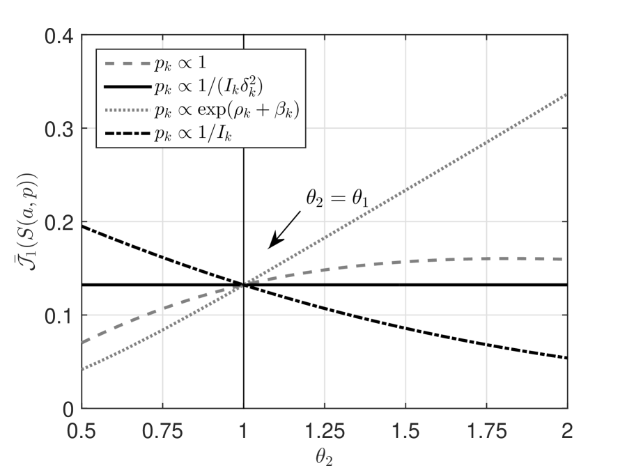
(a) The change occurs in the first sensor.

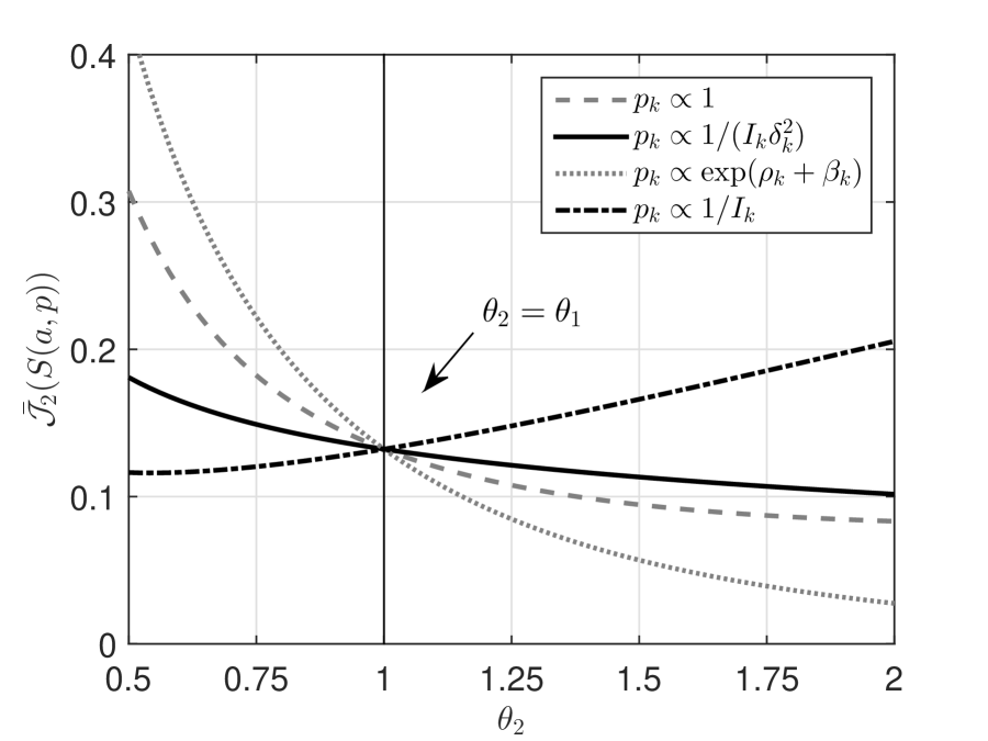
(b) The change occurs in the second sensor.

Figure 1: The horizontal axis in both graphs represents $\theta_{2}$, the post-change mean in the second sensor when it is the one affected by the change. The post-change mean in the first sensor, $\theta_{1}$, when this is the one affected by the change, is fixed to 1. The vertical axis in (a) (resp. (b)) represents the asymptotic relative performance loss of the multichart CUSUM when the first (resp. second) sensor is affected.

5 A simulation study

5.1 Description

In this section we present the results of a simulation study whose main goal is to compare the GLR-CUSUM, $S$, given by (11), the mixture-based CUSUM rules, $\tilde{S}$ and $\hat{S}$, given by (14) and (24), respectively, and the SUM-CUSUM, $M$, defined in (27). We set $K=5$ and $h_{k}=\mathcal{N}(0,1)$, $g_{k}=\mathcal{N}(1,1)$. That is, all sensors initially observe iid Gaussian observations with variance $1$, and at the time of the change the mean changes from $0$ to $1$ in an unknown subset of these sensors. For our comparisons to be fair, we need to guarantee that all detection rules have access to the same amount of prior information. We consider the following regimes: (i) no prior information ($\mathcal{P}=\overline{\mathcal{P}}_{K})$; (ii) knowing that at most $L$ sensors can be affected ($\mathcal{P}=\overline{\mathcal{P}}_{L}$), where $1\leq L\leq K$.

For the implementation of $S$ and $\tilde{S}$ we follow the first approach described in Subsection 2.4. For the implementation of $\hat{S}$ we use the second approach, together with the adaptive-window based on regeneration times (15).

For all detection rules we have considered in this work, the worst case scenario is when the change occurs at time $0$. Thus, when the actual affected subset is $\mathcal{A}$, in order to compute the worst-case detection delay of each rule we simply need to simulate it under ${\sf P}_{0}^{\mathcal{A}}$.

In order to have a direct comparison of the various detection rules and also to illustrate the second-order asymptotic optimality property, we plot the additional number of observations required by each rule in order to detect the change relative to the optimal CUSUM test for which the affected subset is known in advance. Thus, if $T$ represents a generic detection rule and $\mathcal{A}$ the true subset of affected sensors, we plot $\operatorname{{\sf E}}_{0}^{\mathcal{A}}[T]-\operatorname{{\sf E}}_{0}^{\mathcal{A}}[S^{\mathcal{A}}]$ against $\text{ARL}[T]:=\operatorname{{\sf E}}_{\infty}[T]$ for various threshold choices. In order to illustrate the first-order asymptotic optimality property, we plot the ratio $\operatorname{{\sf E}}_{0}^{\mathcal{A}}[T]/\operatorname{{\sf E}}_{0}^{\mathcal{A}}[S^{\mathcal{A}}]$ against $\text{ARL}[T]=\operatorname{{\sf E}}_{\infty}[T]$ again for various threshold choices. In Table 1, we present numerical results for all detection rules when we choose their thresholds so that their target for the expected time to false alarm is $\gamma=10^{5}$. Standard errors are given based on $50,000$ Monte Carlo simulation runs.

5.2 Results

5.2.1 No prior information

We present the results that correspond to the case of no prior information in Fig. 2–Fig. 3, illustrating the notion of first-order and second-order asymptotic optimality with respect to class  $\overline{\mathcal{P}}_{K}$, respectively. We see that when $2$ sensors are affected, the mixture-based CUSUM procedures are slightly worse than the GLR-CUSUM, whereas when $4$ sensors are affected, the mixture CUSUMs take the lead. In both cases the proposed schemes perform much better than SUM-CUSUM, $M(5)$, whose inflicted performance loss (relative to the optimal performance) increases much faster as $\gamma$ increases. Nevertheless, its ratio over the optimal performance decreases, which supports the result that SUM-CUSUM is first-order asymptotically optimal.

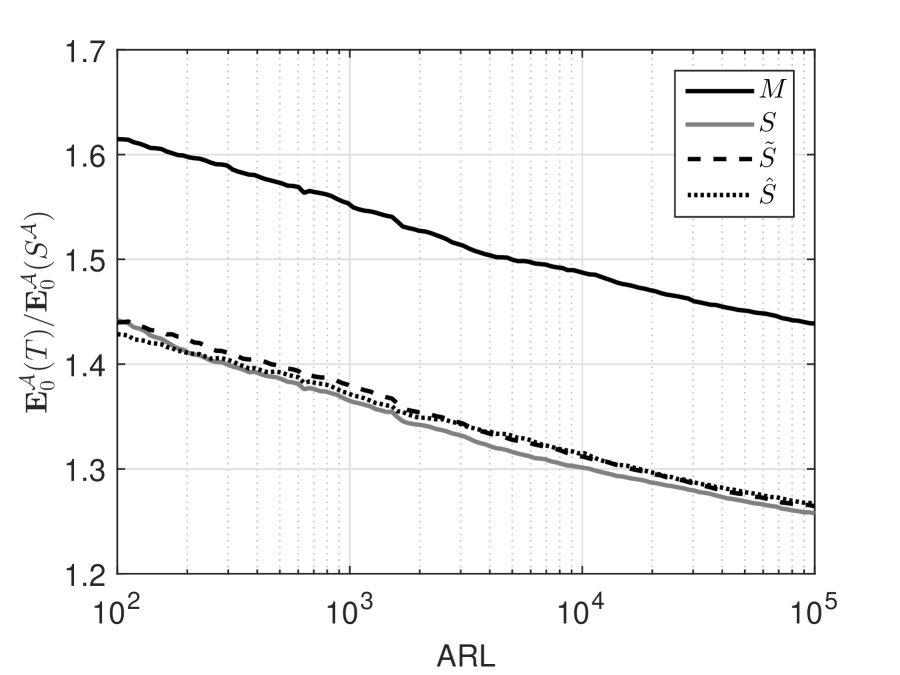
(a) $2$ affected sensors.

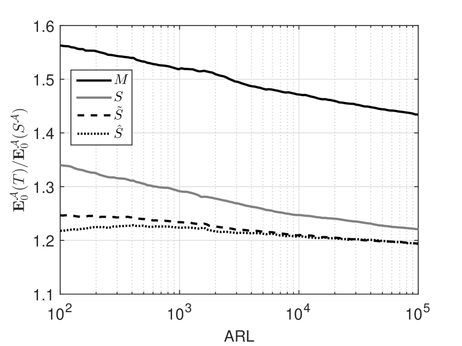
(b) $4$ affected sensors.

Figure 2: First-order asymptotic optimality is illustrated in the case of no prior information. The performance ratio (vertical axis) of each rule is plotted against the expected time for a false alarm (horizontal axis).

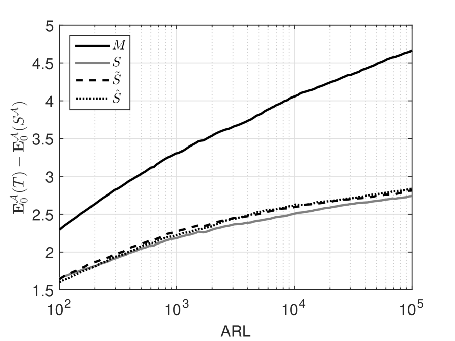
(a) $2$ affected sensors.

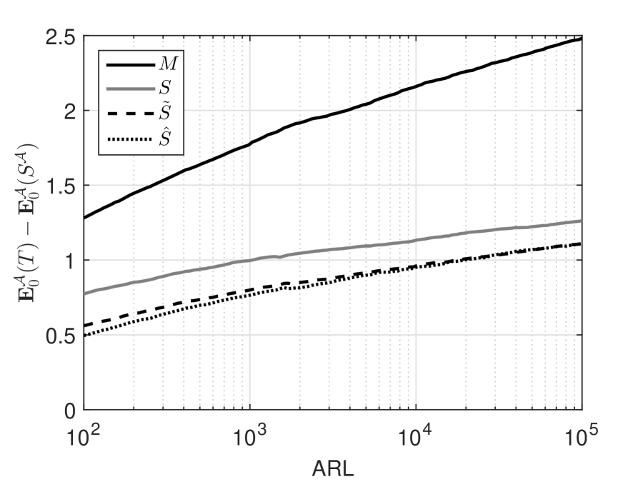
(b) $4$ affected sensors.

Figure 3: Second-order asymptotic optimality is illustrated in the case of no prior information. The performance loss (vertical axis) of each rule is plotted against the expected time for a false alarm (horizontal axis).

5.2.2 An upper bound on the number of affected sensors is known

In Fig. 4–5 we assume that we know in advance that at most $L$ sensors can be affected and we compare the GLR-CUSUM procedure, $S$, the mixture-based CUSUM procedures, $\tilde{S}$ and $\hat{S}(L/(2K))$, and the scalable scheme $M(L)$. Again, we see that $M(L)$ performs uniformly worse than the proposed schemes in all cases.

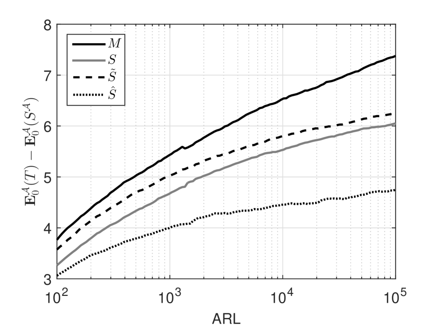
(a) $1$ sensor actually affected

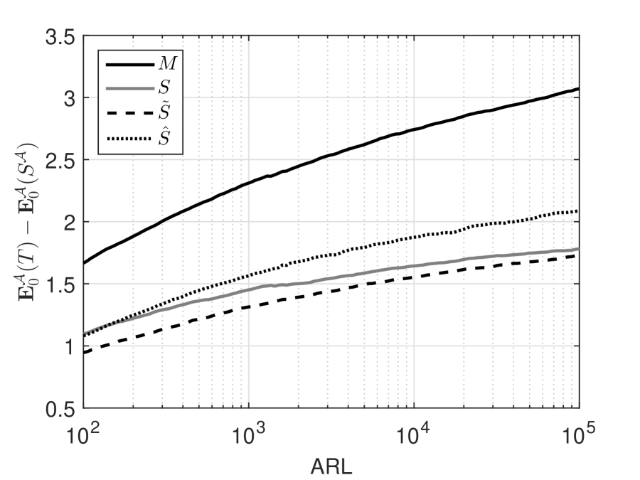
(b) $3$ sensors actually affected

Figure 4: Second-order asymptotic optimality illustrated when it is known that at most $3$ sensors may be affected. The performance loss (vertical axis) of each rule is plotted against the expected time for a false alarm (horizontal axis).

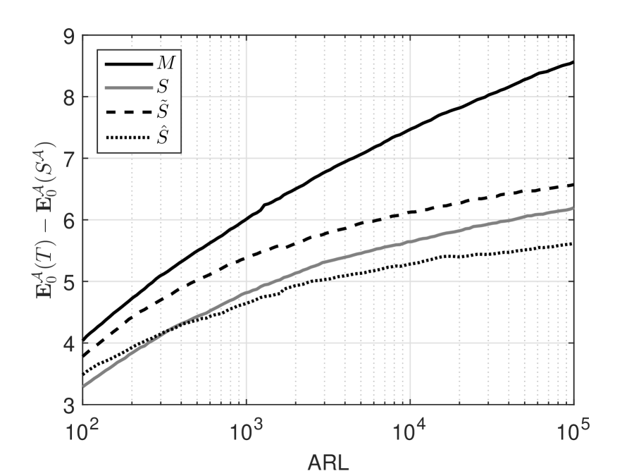
(a) $1$ sensor actually affected

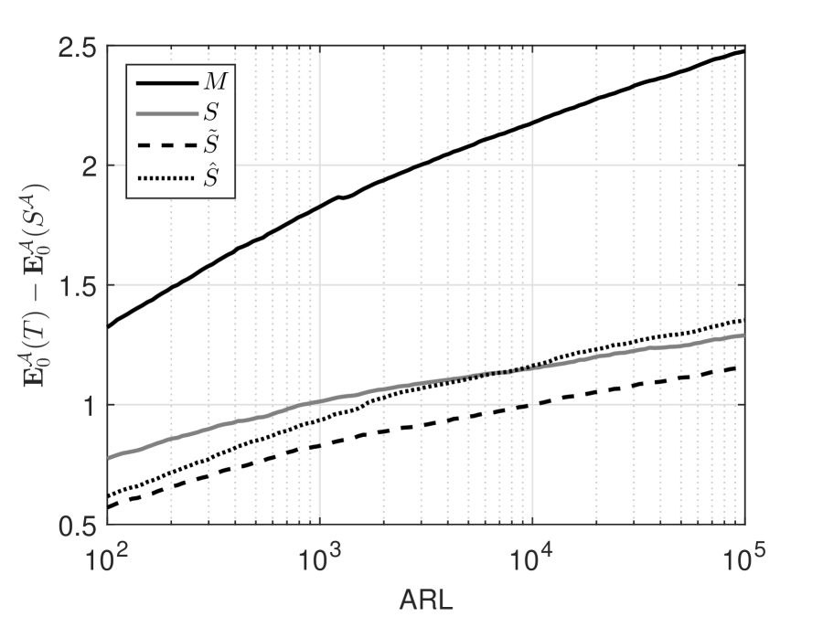
(b) $4$ sensors actually affected

Figure 5: Second-order asymptotic optimality illustrated when it is known that at most $4$ sensors may be affected. The performance loss (vertical axis) of each rule is plotted against the expected time for a false alarm (horizontal axis)

Table 1: Performance of various procedures when $|\mathcal{A}|$ sensors are affected. The thresholds are selected so that the expected time to false alarm is approximately $\gamma=10^{5}$ .

   $|\mathcal{A}|$ $b$ $\operatorname{{\sf E}}_{\infty}(T)$ $\operatorname{{\sf SE}}$ $\operatorname{{\sf E}}_{0}^{\mathcal{A}}(T)$ $\operatorname{{\sf SE}}$ $S_{b}^{\mathcal{A}}$ $2$ $9.88$ $100090$ $450$ $10.64$ $0.02$ $M_{b}(5)$ $2$ $17.1$ $100010$ $455$ $15.30$ $0.03$ $M_{b}(2)$ $2$ $14.2$ $100065$ $450$ $14.21$ $0.03$ $\hat{S}_{b}(0.5)$ $2$ $9.85$ $100065$ $450$ $13.47$ $0.03$ $\hat{S}_{b}(0.2)$ $2$ $9.35$ $100105$ $450$ $13.57$ $0.03$ $\tilde{S}_{b}(\overline{\mathcal{P}}_{5})$ $2$ $9.91$ $100105$ $450$ $13.45$ $0.03$ $\tilde{S}_{b}(\overline{\mathcal{P}}_{2})$ $2$ $9.86$ $100115$ $465$ $13.12$ $0.03$ $S_{b}(\overline{\mathcal{P}}_{5})$ $2$ $9.58$ $100005$ $445$ $13.38$ $0.03$ $S_{b}(\overline{\mathcal{P}}_{2})$ $2$ $9.78$ $100005$ $460$ $13.15$ $0.03$ $S_{b}^{\mathcal{A}}$ $3$ $9.94$ $100065$ $450$ $7.369$ $0.02$ $M_{b}(5)$ $3$ $17.1$ $100010$ $455$ $10.59$ $0.02$ $M_{b}(3)$ $3$ $15.9$ $100025$ $450$ $10.44$ $0.02$ $\hat{S}_{b}(0.5)$ $3$ $9.85$ $100065$ $450$ $9.040$ $0.02$ $\hat{S}_{b}(0.3)$ $3$ $9.63$ $100075$ $460$ $9.458$ $0.02$ $\tilde{S}_{b}(\overline{\mathcal{P}}_{5})$ $3$ $9.91$ $100105$ $450$ $9.054$ $0.02$ $\tilde{S}_{b}(\overline{\mathcal{P}}_{3})$ $3$ $9.90$ $100115$ $450$ $9.098$ $0.02$ $S_{b}(\overline{\mathcal{P}}_{5})$ $3$ $9.58$ $100005$ $445$ $9.136$ $0.02$ $S_{b}(\overline{\mathcal{P}}_{3})$ $3$ $9.67$ $100060$ $450$ $9.150$ $0.02$ $S_{b}^{\mathcal{A}}$ $4$ $9.93$ $100010$ $450$ $5.716$ $0.02$ $M_{b}(5)$ $4$ $17.1$ $100010$ $455$ $8.197$ $0.02$ $M_{b}(4)$ $4$ $16.8$ $100050$ $450$ $8.192$ $0.02$ $\hat{S}_{b}(0.5)$ $4$ $9.85$ $100065$ $450$ $6.821$ $0.02$ $\hat{S}_{b}(0.4)$ $4$ $9.75$ $100050$ $450$ $7.068$ $0.02$ $\tilde{S}_{b}(\overline{\mathcal{P}}_{5})$ $4$ $9.91$ $100105$ $450$ $6.826$ $0.02$ $\tilde{S}_{b}(\overline{\mathcal{P}}_{4})$ $4$ $9.91$ $100070$ $450$ $6.870$ $0.02$ $S_{b}(\overline{\mathcal{P}}_{5})$ $4$ $9.58$ $100005$ $445$ $6.977$ $0.02$ $S_{b}(\overline{\mathcal{P}}_{4})$ $4$ $9.60$ $100010$ $450$ $7.006$ $0.02$  

6 Conclusions

We considered a generalized multisensor sequential change detection problem, in which a number of possibly correlated sensors are monitored on line, a global parameter vector determines their joint distribution and there is a change in an unknown subset of the components of this parameter vector. In this context, we established a strong asymptotic optimality property for various CUSUM-based detection rules. In the special case that the sensors are independent and only a subset of them is affected by the change, we proposed feasible versions of the above procedures. We showed using simulation experiments that the proposed detection rules always outperform scalable detection rules, such as the one proposed in [10], and we argued that this phenomenon can be explained theoretically by the fact that the latter scheme enjoys a weaker form of asymptotic optimality. Moreover, we proposed a modification of a detection rule in [14] that is able to incorporate prior information. Finally, we considered the design of the multichart CUSUM in the special case that the change is known to affect exactly one sensor.

7 Acknowledgments

We would like to thank Drs. Alexander Tartakovsky, George Moustakides, Venu Veeravalli and Emmanuel Yashchin for stimulating discussions and helpful suggestions, as well as the two referees whose comments helped us improve significantly an earlier version of this paper. The work of the first author was supported by the US National Science Foundation under Grant CCF 1514245, as well as by a collaboration grant from the Simons Foundation.

Appendix

Proof of Theorem 1.

From the definition of the three detection rules it is clear that $\tilde{S}_{b}\leq S_{b}$ and $\bar{S}_{b}\leq S_{b}$, therefore for any $b$ and $\mathcal{A}$ we have:

$$\mathcal{J}_{\mathcal{A}}[\bar{S}_{b}]\leq\mathcal{J}_{\mathcal{A}}[S_{b}]\quad\text{and}\quad\operatorname{{\sf E}}_{\infty}[S_{b}]\geq\operatorname{{\sf E}}_{\infty}[\bar{S}_{b}]$$

and

$$\mathcal{J}_{\mathcal{A}}[\tilde{S}_{b}]\leq\mathcal{J}_{\mathcal{A}}[S_{b}]\quad\text{and}\quad\operatorname{{\sf E}}_{\infty}[S_{b}]\geq\operatorname{{\sf E}}_{\infty}[\tilde{S}_{b}].$$

Consequently, in order to prove (i), it suffices to show that for any $b>0$

$$\operatorname{{\sf E}}_{\infty}[\bar{S}_{b}]\geq e^{b}\quad\text{and}\quad\operatorname{{\sf E}}_{\infty}[\tilde{S}_{b}]\geq e^{b},$$ (37)

and in order to establish (ii), it suffices to show that as $b\rightarrow\infty$

$$\mathcal{J}_{\mathcal{A}}[S_{b}]\leq\frac{b}{I_{\mathcal{A}}}+{\mathcal{O}}(1).$$ (38)

(i) In order to prove the first inequality in (37), we introduce the mixture probability measure

$$\bar{{\sf P}}:=\sum_{\mathcal{A}\in\mathcal{P}}p_{\mathcal{A}}{\sf P}_{0}^{\mathcal{A}},$$

and denote by $\overline{\operatorname{{\sf E}}}$ the corresponding expectation. The mixture-based CUSUM rule $\bar{S}_{b}$ results from repeated application, in the spirit of Lorden’s [8] construction, of the one-sided sequential test:

$$\bar{T}_{b} :=\inf\left\{t\geq 0:\bar{\Lambda}_{t}\geq e^{b}\right\},$$

where $\bar{\Lambda}$ is the likelihood ratio process of $\bar{{\sf P}}$ versus ${\sf P}_{\infty}$, i.e.,

$$\bar{\Lambda}_{t}:=\frac{d\bar{{\sf P}}}{d{\sf P}_{\infty}}({\mathcal{F}}_{t})=\sum_{\mathcal{A}\in\mathcal{P}}p_{\mathcal{A}}\Lambda_{t}^{\mathcal{A}},\quad t\in\mathbb{N}.$$

Consequently, from [8, Th. 2] it follows that for every $b>0$ we have

$$\operatorname{{\sf E}}_{\infty}[\bar{S}_{b}]\geq\frac{1}{{\sf P}_{\infty}(\bar{T}_{b}<\infty)},$$

and from Wald’s likelihood ratio identity we obtain

$${\sf P}_{\infty}(\bar{T}_{b}<\infty) =\overline{\operatorname{{\sf E}}}\left[\bar{\Lambda}^{-1}_{T_{b}}\,\mathchoice{\rm 1\mskip-4.2mul}{\rm 1\mskip-4.2mul}{\rm 1\mskip-4.6mul}{\rm 1\mskip-5.2mul}_{\{\bar{T}_{b}<\infty\}}\right]\leq e^{-b},$$

which completes the proof of the first inequality in (37). In order to establish the second inequality, we introduce for each subset $\mathcal{A}\in\mathcal{P}$ the corresponding Shiryaev-Roberts statistic

$$R_{t}^{\mathcal{A}}:=\sum_{s=0}^{t-1}\exp(Z_{t}^{\mathcal{A}}-Z_{s}^{\mathcal{A}}),\quad R_{0}^{\mathcal{A}}:=0$$

and observe that

$$R_{t}^{\mathcal{A}}\geq\max_{0\leq s<t}\exp(Z_{t}^{\mathcal{A}}-Z_{s}^{\mathcal{A}})=\exp(\tilde{Y}_{t}^{\mathcal{A}}).$$

We also introduce the mixture Shiryaev-Roberts statistic $R_{t}:=\sum_{\mathcal{A}\in\mathcal{P}}p_{\mathcal{A}}R_{t}^{\mathcal{A}}$ and the corresponding stopping time $\mathcal{R}_{b}:=\inf\left\{t\geq 0:R_{t}\geq e^{b}\right\}.$ Then, for any $b>0$ we obtain

$$\tilde{S}_{b} =\inf\left\{t\in\mathbb{N}:\sum_{\mathcal{A}\in\mathcal{P}}p_{\mathcal{A}}\exp(\tilde{Y}_{t}^{\mathcal{A}})\geq e^{b}\right\}$$

$$\geq\inf\left\{t\in\mathbb{N}:\sum_{\mathcal{A}\in\mathcal{P}}p_{\mathcal{A}}R_{t}^{\mathcal{A}}\geq e^{b}\right\}=\mathcal{R}_{b},$$

thus, it suffices to show that $\operatorname{{\sf E}}_{\infty}[\mathcal{R}_{b}]\geq e^{b}$. In order to see this, note that for any $b$ and $t$ we have $0\leq R_{t}<e^{b}$ on the event $\{\mathcal{R}_{b}>t\}$, therefore

$$\int_{\{\mathcal{R}_{b}>t\}}|R_{t}-t|\,d{\sf P}_{\infty} \leq\int_{\{\mathcal{R}_{b}>t\}}R_{t}\,d{\sf P}_{\infty}+\int_{\{\mathcal{R}_{b}>t\}}t\,d{\sf P}_{\infty}$$

$$\leq e^{b}\,{\sf P}_{\infty}(\mathcal{R}_{b}>t)+\int_{\{\mathcal{R}_{b}>t\}}\mathcal{R}_{b}\,d{\sf P}_{\infty}.$$

For any given $b$, the upper bound goes to 0 as $t\rightarrow\infty$ as long as $\operatorname{{\sf E}}_{\infty}[\mathcal{R}_{b}]<\infty$. But this can be assumed without any loss of generality, since otherwise the desired inequality holds trivially. Therefore, we can apply the optional sampling theorem to the ${\sf P}_{\infty}$-martingale $\{R_{t}-t\}_{t\in\mathbb{N}}$ and the stopping time $\mathcal{R}_{b}$ and obtain $\operatorname{{\sf E}}_{\infty}[\mathcal{R}_{b}]=\operatorname{{\sf E}}_{\infty}[R_{\mathcal{R}_{b}}]\geq e^{b},$ where the inequality holds from the definition of the stopping rule $\mathcal{R}_{b}$. This completes the proof of the second inequality in (37).

(ii) For any $b>0$ and $\mathcal{A}\in\mathcal{P}$, from the definition of $S_{b}$ in (11) it follows that $S_{b}\leq S_{b-\log p_{\mathcal{A}}}^{\mathcal{A}}$, where $S_{b-\log p_{\mathcal{A}}}^{\mathcal{A}}$ is the CUSUM rule defined in (5) with threshold $b-\log p_{\mathcal{A}}$. Consequently, as $b\rightarrow\infty$ we have

$$\mathcal{J}_{\mathcal{A}}[S_{b}] \leq\frac{b-\log p_{\mathcal{A}}}{I_{\mathcal{A}}}+{\mathcal{O}}(1)=\frac{b}{I_{\mathcal{A}}}+{\mathcal{O}}(1),$$

which completes the proof of (38).

∎

Proof of Proposition 1.

Fix $b>0$ and $\mathcal{A}\in\mathcal{P}$. (i) We will first prove the result for the GLR-CUSUM, $S_{b}$. On the event $\{S_{b}>\nu\}$ we have

$$S_{b}=\inf\left\{t>\nu:\max_{\mathcal{B}\in\mathcal{P}}\left(Y_{t}^{\mathcal{B}}-Y_{\nu}^{\mathcal{B}}+Y_{\nu}^{\mathcal{B}}+\log p_{\mathcal{B}}\right)\geq b\right\}.$$

For each $\mathcal{B}\in\mathcal{P}$, $\{Y_{t}^{\mathcal{B}}-Y_{\nu}^{\mathcal{B}}\}_{t>\nu}$ depends only on the post-change observations. Therefore, the detection statistic depends on the pre-change observations only through the non-negative random variables $Y_{\nu}^{\mathcal{B}}$, $\mathcal{B}\in\mathcal{P}$. Moreover, the detection statistic is increasing in these quantities, which means that, for any possible change point $\nu$, the worst-possible scenario for the history of observations up to $\nu$ is that $Y_{\nu}^{\mathcal{B}}=0$ for every $\mathcal{B}\in\mathcal{P}$:

$$\operatorname*{ess\,sup}\operatorname{{\sf E}}^{\mathcal{A}}_{\nu}[\left(S_{b}-\nu\right)^{+}|\mathcal{F}_{\nu}] =\operatorname{{\sf E}}^{\mathcal{A}}_{\nu}[\left(S_{b}-\nu\right)^{+}|\,Y^{\mathcal{B}}_{\nu}=0,\,\forall\,\mathcal{B}\in\mathcal{P}].$$

However, when $Y_{\nu}^{\mathcal{B}}=0$ for every $\mathcal{B}\in\mathcal{P}$, each sequence $\{Y_{t}^{\mathcal{B}}-Y_{\nu}^{\mathcal{B}}\}_{t\geq\nu}$ under ${\sf P}_{\nu}^{\mathcal{A}}$ has the same distribution as $\{Y^{\mathcal{B}}_{t}\}_{t\geq 0}$ under ${\sf P}_{0}^{\mathcal{A}}$. Thus, for every change-point $\nu$ we have

$$\operatorname{{\sf E}}^{\mathcal{A}}_{\nu}[\left(S_{b}-\nu\right)^{+}|\,Y^{\mathcal{B}}_{\nu}=0,\,\forall\,\mathcal{B}\in\mathcal{P}] =\operatorname{{\sf E}}_{0}^{\mathcal{A}}[S_{b}],$$

which proves that $\mathcal{J}_{\mathcal{A}}[S_{b}]=\operatorname{{\sf E}}_{0}^{\mathcal{A}}[S_{b}]$.

(ii) In order to prove the corresponding result for $\bar{S}_{b}$, we note that on the event $\{\bar{S}_{b}>\nu\}$ we have

$$\bar{S}_{b} =\inf\left\{t>\nu:\max_{0\leq s\leq t}\sum_{\mathcal{B}\in\mathcal{P}}p_{\mathcal{B}}\exp(Z_{t}^{\mathcal{B}}-Z_{s}^{\mathcal{B}})\geq e^{b}\right\}$$

$$\leq\inf\left\{t>\nu:\max_{\nu\leq s\leq t}\sum_{\mathcal{B}\in\mathcal{P}}p_{\mathcal{B}}\exp(Z_{t}^{\mathcal{B}}-Z_{s}^{\mathcal{B}})\geq e^{b}\right\}$$

$$:=\bar{S}_{b}^{(\nu)}.$$

For every change point $\nu$, $\bar{S}_{b}^{(\nu)}$ under ${\sf P}_{\nu}^{\mathcal{A}}$ has the same distribution as $\bar{S}_{b}$ under ${\sf P}_{0}^{\mathcal{A}}$ and is independent of $\mathcal{F}_{\nu}$. Therefore,

$$\operatorname{{\sf E}}_{\nu}^{\mathcal{A}}\left[(\bar{S}_{b}-\nu)^{+}|\mathcal{F}_{\nu}\right] \leq\operatorname{{\sf E}}_{\nu}^{\mathcal{A}}[\bar{S}_{b}^{(\nu)}]=\operatorname{{\sf E}}_{0}^{\mathcal{A}}[\bar{S}_{b}],$$

which proves that $\mathcal{J}_{\mathcal{A}}[\bar{S}_{b}]\leq\operatorname{{\sf E}}_{0}^{\mathcal{A}}[\bar{S}_{b}]$, and consequently $\mathcal{J}_{\mathcal{A}}[\bar{S}_{b}]=\operatorname{{\sf E}}_{0}^{\mathcal{A}}[\bar{S}_{b}]$.

(iii) Finally, on the event $\{\tilde{S}_{b}>\nu\}$ we have

$$\tilde{S}_{b} =\inf\left\{t>\nu:\sum_{\mathcal{B}\in\mathcal{P}}p_{\mathcal{B}}\,\exp\{\tilde{Y}_{t}^{\mathcal{B}}\}\geq b\right\}$$

$$=\inf\left\{t>\nu:\sum_{\mathcal{B}\in\mathcal{P}}p_{\mathcal{B}}\,\exp\{\tilde{Y}_{t}^{\mathcal{B}}-\tilde{Y}_{\nu}^{\mathcal{B}}+\tilde{Y}_{\nu}^{\mathcal{B}}\}\geq b\right\}.$$

Fix $\mathcal{B}\in\mathcal{P}$. When $\tilde{Y}_{\nu}^{\mathcal{B}}<0$, then from recursion (7) it follows that $\{\tilde{Y}_{t}^{\mathcal{B}}\}_{t>\nu}$ is independent of $\mathcal{F}_{\nu}$ and that its distribution under ${\sf P}_{\nu}^{\mathcal{A}}$ is the same as that of $\{\tilde{Y}_{t}^{\mathcal{B}}\}_{t>0}$ under ${\sf P}_{0}^{\mathcal{A}}$. When $\tilde{Y}_{\nu}^{\mathcal{B}}\geq 0$, a similar argument as in (i) shows that the worst case is $\tilde{Y}_{\nu}^{\mathcal{B}}=0$. Thus, we conclude that $\mathcal{J}_{\mathcal{A}}[\tilde{S}_{b}]=\operatorname{{\sf E}}_{0}^{\mathcal{A}}[\tilde{S}_{b}]$.

∎

Proof of Proposition 2.

Recall the notation $C(\mathcal{P}):=\sum_{\mathcal{B}\in\mathcal{P}}p^{|\mathcal{B}|}$.

(i) We observe that $\log C(\mathcal{P}_{L})=L\log p+\log|\mathcal{P}_{L}|$ and

$$\max_{\mathcal{A}\in\mathcal{P}_{L}}\sum_{k\in\mathcal{A}}\left(Z_{t}^{k}-Z_{s}^{k}+\log p\right) =\sum_{k=1}^{L}\left(Z_{s:t}^{(k)}+\log p\right),$$

which proves (22). Moreover, we observe that $\log C(\overline{\mathcal{P}}_{L})=\log\left(\sum_{k=1}^{L}|\mathcal{P}_{k}|\,p^{k}\right)$ and that

$$\max_{\mathcal{A}\in\mathcal{P}}\sum_{k\in\mathcal{A}}\left(Z_{t}^{k}-Z_{s}^{k}+\log p\right)=\sum_{k=1}^{L}\left(Z_{s:t}^{(k)}+\log p\right)^{+}$$

whenever there is at least one $k$ such that $Z_{t}^{k}-Z_{s}^{k}+\log p>0$. On the other hand, if $Z_{t}^{k}-Z_{s}^{k}+\log p\leq 0$ for every $1\leq k\leq K$, the detection statistic cannot reach a positive threshold, which completes the proof of (23).

(ii) We observe that for any $\pi\in(0,1)$ and $p=\pi/(1-\pi)$ we have

$$\prod_{k=1}^{K}\left(1-\pi+\pi\,\frac{\Lambda_{t}^{k}}{\Lambda_{s}^{k}}\right)$$

$$=(1-\pi)^{K}+\sum_{\mathcal{A}\in\overline{\mathcal{P}}_{K}}(1-\pi)^{K-|\mathcal{A}|}\,\pi^{|\mathcal{A}|}\prod_{k\in\mathcal{A}}\frac{\Lambda_{t}^{k}}{\Lambda_{s}^{k}}$$

$$=(1-\pi)^{K}\left[1+\sum_{\mathcal{A}\in\overline{\mathcal{P}}_{K}}p^{|\mathcal{A}|}\,\frac{\Lambda_{t}^{\mathcal{A}}}{\Lambda_{s}^{\mathcal{A}}}\right],$$

which proves (24).

∎

Proof of Theorem 2.

(i) Fix $b$. We need to show that

$$\operatorname{{\sf E}}_{\infty}[\hat{S}_{b}(\pi)] \geq e^{b}\quad\text{and}\quad\operatorname{{\sf E}}_{\infty}[\check{S}_{b}(\pi)]\geq\frac{e^{b}}{|\overline{\mathcal{P}}_{K}|},$$ (39)

where $\pi\in(0,1)$ in the first and $\pi\in(0,1]$ in the second inequality. In order to prove the first inequality, we recall that $\hat{S}_{b}(\pi)$ can be obtained with the repeated application of the one-sided sequential test $\hat{T}_{b}(\pi)$, defined in (25). Therefore, from [8, Th. 2] it follows that

$$\operatorname{{\sf E}}_{\infty}[\hat{S}_{b}(\pi)]\geq\frac{1}{{\sf P}_{\infty}(\hat{T}_{b}(\pi)<\infty)}$$

and from Wald’s likelihood ratio identity we obtain

$${\sf P}_{\infty}(\hat{T}_{b}(\pi)<\infty) =\hat{\operatorname{{\sf E}}}\left[\exp\left\{-\hat{Z}_{\hat{T}_{b}(\pi)}\right\}\;\mathchoice{\rm 1\mskip-4.2mul}{\rm 1\mskip-4.2mul}{\rm 1\mskip-4.6mul}{\rm 1\mskip-5.2mul}_{\{\hat{T}_{b}(\pi)<\infty\}}\right]\leq e^{-b},$$

where $\hat{Z}$ is the logarithm of the likelihood ratio $\hat{\Lambda}^{\pi}$ defined in (25), i.e.,

$$\hat{Z}_{t} :=\log\hat{\Lambda}_{t}=\sum_{k=1}^{K}\log\left(1-\pi+\pi\,\Lambda_{t}^{k}\right).$$

This completes the proof of the first inequality in (39). In order to prove the second inequality, it suffices to observe that for any $b>0$ and $\pi\in(0,1]$ we have

$$\hat{S}_{b}(\pi)\geq\check{S}_{b}(\pi)\geq\inf\Bigl{\{}t\geq 0:\max_{0\leq s\leq t}\sum_{k=1}^{K}(Z_{t}^{k}-Z_{s}^{k})^{+}\geq b\Bigr{\}}$$

and that the lower bound coincides (up to a constant) with the unweighted GLR-CUSUM in the case of complete uncertainty, that is the detection rule obtained by setting $L=K$ and $\pi=1$ in (23).

(ii) When $\pi=1$, $\check{S}_{b}(\pi)$ coincides with the GLR-CUSUM in the case of complete uncertainty, whose asymptotic optimality has already been established. Therefore, without loss of generality, we assume that $\pi\in(0,1)$. Due to the pathwise inequality $\hat{S}_{b}(\pi)\geq\check{S}_{b}(\pi)$, it suffices to show that for every subset $\mathcal{A}$ we have

$$\mathcal{J}_{\mathcal{A}}[\hat{S}_{b}(\pi)] \leq\frac{b}{I_{\mathcal{A}}}+{\mathcal{O}}(1),$$

where ${\mathcal{O}}(1)$ is a bounded term as $b\rightarrow\infty$. From [8, Th. 2] it follows that $\mathcal{J}_{\mathcal{A}}[\hat{S}_{b}(\pi)]\leq\operatorname{{\sf E}}_{0}^{\mathcal{A}}[\hat{T}_{b}(\pi)]$ for every $b>0$, whereas for every $t$ we observe that

$$\hat{Z}_{t} =\sum_{k=1}^{K}\log\left(1-\pi+\pi\,\exp(Z_{t}^{k})\right)$$

$$\geq\sum_{k\in\mathcal{A}}(Z_{t}^{k}+\log\pi)+\sum_{k\notin\mathcal{A}}\log(1-\pi)$$

$$=Z_{t}^{\mathcal{A}}+c_{\mathcal{A}},$$

where $c_{\mathcal{A}}:=|\mathcal{A}|\,\log\pi+(K-|\mathcal{A}|)\,\log(1-\pi)$. Therefore, $\hat{T}_{b}(\pi)\leq\inf\{t:Z_{t}^{\mathcal{A}}\geq b+c_{\mathcal{A}}\}$ for every $b>0$, and consequently

$$\operatorname{{\sf E}}_{0}^{\mathcal{A}}[\hat{T}_{b}(\pi)] \leq\frac{b+c_{\mathcal{A}}}{I_{\mathcal{A}}}+{\mathcal{O}}(1),$$

which completes the proof. ∎

References

• [1] A. G. Tartakovsky, B. L. Rozovskii, R. B. Blažek, and H. Kim, “A novel approach to detection of intrusions in computer networks via adaptive sequential and batch-sequential change-point detection methods,” IEEE Transactions on Signal Processing, vol. 54, no. 9, pp. 3372–3382, 2006.
• [2] ——, “Detection of intrusions in information systems by sequential changepoint methods (with discussion),” Statistical Methodology, vol. 3, no. 3, pp. 252–340, 2006.
• [3] C. Lévy-Leduc and F. Roueff, “Detection and localization of change-points in high-dimensional network traffic data,” Annals of Applied Statisticss, vol. 3, no. 2, pp. 637–662, 2009.
• [4] C. Sonesson and D. Bock, “A review and discussion of prospective statistical surveillance in public health,” Journal of the Royal Statistical Society. Series A (Statistics in Society), vol. 166, no. 1, pp. 5–21, 2003.
• [5] G. Shmueli and H. Burkom, “Statistical challenges facing early outbreak detection in biosurveillance,” Technometrics, vol. 52, no. 1, pp. 39–51, February 2010.
• [6] E. S. Page, “Continuous inspection schemes,” Biometrika, vol. 41, no. 1, pp. 100–115, 1954.
• [7] G. V. Moustakides, “Optimal stopping times for detecting changes in distributions,” The Annals of Statistics, vol. 14, no. 4, pp. 1379–1387, 1986.
• [8] G. Lorden, “Procedures for reacting to a change in distribution,” The Annals of Mathematical Statistics, vol. 42, no. 6, pp. 1897–1908, 1971.
• [9] A. Tartakovsky, I. Nikiforov, and M. Basseville, Sequential Analysis: Hypothesis Testing and Changepoint Detection.   CRC Press, 2014.
• [10] Y. Mei, “Efficient scalable schemes for monitoring a large number of data streams,” Biometrika, vol. 97, no. 2, pp. 419–433, 2010.
• [11] ——, “Quickest detection in censoring sensor networks,” in IEEE International Symposium on Information Theory, 2011, pp. 2148–2152.
• [12] K. Liu, Y. Mei, and J. Shi, “An adaptive sampling strategy for online high-dimensional process monitoring,” Technometrics, 2015, to appear.
• [13] T. Banerjee and V. V. Veeravalli, “Data-efficient quickest outlying sequence detection in sensor networks.”
• [14] Y. Xie and D. Siegmund, “Sequential multi-sensor change-point detection,” The Annals of Statistics, vol. 41, no. 2, pp. 670–692, 2013.
• [15] Y. C. Chen, T. Banerjee, A. D. Dominguez-Garcia, and V. V. Veeravalli, “Quickest line outage detection and identification,” Power Systems, IEEE Transactions on, vol. PP, no. 99, pp. 1–10, 2015.
• [16] D. Siegmund and E. S. Venkatraman, “Using the generalized likelihood ratio statistic for sequential detection of a change-point,” Annals of Statistics, vol. 23, no. 1, pp. 255–271, 1995.
• [17] V. Raghavan and V. V. Veeravalli, “Quickest change detection of a markov process across a sensor array,” Information Theory, IEEE Transactions on, vol. 56, no. 4, pp. 1961–1981, April 2010.
• [18] M. Ludkovski, “Bayesian quickest detection in sensor arrays,” Sequential Analysis, vol. 31, no. 4, pp. 481–504, 2012.
• [19] O. Hadjiliadis, H. Zhang, and H. V. Poor, “One shot schemes for decentralized quickest change detection,” Information Theory, IEEE Transactions on, vol. 55, no. 7, pp. 3346–3359, July 2009.
• [20] H. Zhang, N. Rodosthenous, and O. Hadjiliadis, “Robustness of the $N$-CUSUM stopping rule in a wiener disorder problem,” The Annals of Applied Probability, 2015, to appear.
• [21] I. V. Nikiforov, “A generalized change detection problem,” Information Theory, IEEE Transactions on, vol. 41, no. 1, pp. 171–187, January 1995.
• [22] ——, “Two strategies in the problem of change detection and isolation,” Information Theory, IEEE Transactions on, vol. 43, no. 2, pp. 770–776, March 1997.
• [23] T. Oskiper and H. V. Poor, “Online activity detection in a multiuser environment using the matrix CUSUM algorithm,” Information Theory, IEEE Transactions on, vol. 48, no. 2, pp. 477–493, February 2002.
• [24] A. G. Tartakovsky, “Multidecision quickest changepoint detection: Previous achievements and open problems,” Sequential Analysis, vol. 27, pp. 201––231, 2008.
• [25] M. Woodroofe, Nonlinear Renewal Theory in Sequential Analysis.   Philadelphia, PA: Society for Industrial and Applied Mathematics, 1982.
• [26] R. A. Khan, “Detecting changes in probabilities of a multi-component process,” Sequential Analysis, vol. 14, no. 4, pp. 375–388, 1995.
• [27] E. Yashchin, “Regenerative likelihood ratio control schemes,” in Frontiers in Statistical Quality Control 11, ser. Frontiers in Statistical Quality Control, S. Knoth and W. Schmid, Eds., 2015, vol. 11.
• [28] ——, “Change-point models in industrial applications,” in Proceedings of the Second World Congress of Nonlinear Analysts, vol. 30, no. 7, December 1997, pp. 3997–4006.
• [29] ——, “Likelihood ratio methods for monitoring parameters of a nested random effect model,” Journal of the American Statistical Association, vol. 90, no. 430, pp. 729–738, June 1995.