Vector form factor of the pion in chiral effective field theory

Abstract

The vector form factor of the pion is calculated in the framework of chiral effective field theory with vector mesons included as dynamical degrees of freedom. To construct an effective field theory with a consistent power counting, the complex-mass scheme is applied.

I Introduction

Chiral perturbation theory (ChPT) is a well-established low-energy effective field theory (EFT) of quantum chromodynamics in the vacuum sector Weinberg:1978kz ; Gasser:1984yg . The extension of this method to also include heavy degrees of freedom beyond the Goldstone bosons is a non-trivial task, which requires both the construction of the relevant most general Lagrangian and a suitable renormalization procedure, resulting in a self-consistent expansion scheme for observables. While for the nucleon and the $\Delta(1232)$ resonance the problem of a self-consistent momentum expansion was solved using various approaches (see, e.g., Refs. Bernard:2007zu ; Scherer:2009bt for a review), the treatment of the $\rho$ meson is more complicated. This is mainly due to the fact that the $\rho$ meson decays into two pions, with vanishing masses in the chiral limit. As a consequence of this decay mode, loop diagrams, when evaluated at energies of the order of the $\rho$-meson mass, develop large power-counting-violating imaginary parts. These parts cannot be absorbed in the redefinition of the parameters of the Lagrangian, as long as the usual renormalization procedure is used. Despite this feature, the heavy-particle approach was considered in Refs. Jenkins:1995vb ; Bijnens:1996kg ; Bijnens:1997ni ; Bijnens:1997rv ; Bijnens:1998di , treating the vector mesons as heavy static matter fields.

A self-consistent solution to the power-counting problem for chiral EFT with explicit vector-meson degrees of freedom is provided by the complex-mass scheme (CMS) Stuart:1990 ; Denner:1999gp ; Denner:2006ic ; Denner:2005fg ; Actis:2006rc ; Actis:2008uh ; Denner:2014zga , which is an extension of the on-mass-shell renormalization scheme to unstable particles. As applications of this approach in chiral EFT with heavy degrees of freedom, the masses and widths of the $\rho$ meson and the Roper resonance were discussed in Refs. Djukanovic:2009zn ; Djukanovic:2010zz , respectively, as well as electromagnetic properties in Refs.  Bauer:2012at ; Djukanovic:2013mka ; Bauer:2014cqa . Different approaches to the inclusion of spin-1 fields have been discussed in, for example, Refs. Rosell:2004mn ; Bruns:2004tj ; Bruns:2008 ; Leupold:2009nv ; Terschluesen:2010ik .

In the present work, we consider the vector form factor of the pion in the time-like region up to $q^{2}\sim 1\,{\rm GeV^{2}}$ in chiral EFT with vector mesons as dynamical degrees of freedom using the CMS. Historically, the existence of a neutral vector meson with isospin zero—nowadays called the $\omega$ meson—was predicted by Nambu Nambu:1957vw to explain the electromagnetic structure of the nucleon. An isoscalar piece was needed to compensate the contribution to the mean square charge radii originating from the pion cloud. Shortly afterwards, Frazer and Fulco Frazer:1959gy realized that, within a dispersion-theoretical treatment of the form factors, an isovector resonance would explain some features of the isovector electromagnetic form factors of the nucleon. The concept of the $\rho$-meson dominance model of the pion form factor was established by Gell-Mann and Zachariasen GellMann:1961tg . For an overview of the vector-meson dominance hypothesis, see Refs. Sakurai:1969 ; Feynman:1972 . In recent years, the pion vector form factor has attracted considerable interest, in particular because of its impact on the determination of the hadronic contribution to the anomalous magnetic moment of the muon Actis:2010gg . From the theoretical side, numerous descriptions of the pion vector form factor exist. For example, in Ref. Brandt:2013dua the pion vector form factor has been studied in the space-like region within lattice QCD and next-to-next-to-leading-order ChPT, while a new approach to the parametrization of the pion vector form factor has been presented in Ref. Hanhart:2012wi .

In this work, we fit the parameters of the effective theory to the $\tau$ decay and describe the pion form factor data. However, to describe the data from $e^{+}e^{-}\to\pi^{+}\pi^{-}$ process we need to take into account the isospin symmetry breaking. This is done by including the $\rho^{0}$-$\omega$-$\gamma$ mixing.

II Lagrangian

To begin with, we specify the Lagrangian of pions ($\pi_{a}$) and $\rho$ mesons ($\rho^{\mu}_{a}$) relevant for the calculation of the vector form factor of the pion Djukanovic:2009zn ; Ecker:1989yg :

$${\cal L} =\frac{F^{2}}{4}\,{\rm Tr}\left[D_{\mu}U\left(D^{\mu}U\right)^{\dagger}\right]+\frac{F^{2}\,M^{2}}{4}\,{\rm Tr}\left(U^{\dagger}+U\right)$$

$$\quad+i\,\frac{l_{6}}{2}\,\text{Tr}\left[f_{R\mu\nu}D^{\mu}U(D^{\nu}U)^{\dagger}+f_{L\mu\nu}(D^{\mu}U)^{\dagger}D^{\nu}U\right]$$

$$\quad-\frac{1}{2}\,{\rm Tr}\left(\rho_{\mu\nu}\rho^{\mu\nu}\right)+\left[M_{\rho}^{2}+\frac{c_{x}\,M^{2}\,{\rm Tr}\left(U^{\dagger}+U\right)}{4}\right]{\rm Tr}\left[\left(\rho_{\mu}-\frac{i\,\Gamma_{\mu}}{g}\right)\left(\rho^{\mu}-\frac{i\,\Gamma^{\mu}}{g}\right)\right]$$

$$\quad+i\,d_{x}{\rm Tr}\left[\rho^{\mu\nu}\Gamma_{\mu\nu}\right]-\frac{f_{V}}{\sqrt{2}}{\rm Tr}\left\{\rho_{\mu\nu}f^{\mu\nu}_{+}\right\}+\cdots,$$ (1)

where the individual elements are defined as

$$U =u^{2}={\rm exp}\left(\frac{i\tau_{a}\pi_{a}}{F}\right),$$

$$D_{\mu}U =\partial_{\mu}U-iv_{\mu}U+iUv_{\mu},$$

$$f_{R\mu\nu} =f_{L\mu\nu}=\partial_{\mu}v_{\nu}-\partial_{\nu}v_{\mu},$$

$$\rho_{\mu} =\frac{\tau_{a}\rho_{a\mu}}{2},$$

$$\rho_{\mu\nu} =\partial_{\mu}\rho_{\nu}-\partial_{\nu}\rho_{\mu}-ig\left[\rho_{\mu},\rho_{\nu}\right],$$

$$\Gamma_{\mu} =\frac{1}{2}\left[u^{\dagger}\partial_{\mu}u+u\partial_{\mu}u^{\dagger}-i\left(u^{\dagger}v_{\mu}u+uv_{\mu}u^{\dagger}\right)\right],$$

$$\Gamma_{\mu\nu} =\partial_{\mu}\Gamma_{\nu}-\partial_{\nu}\Gamma_{\mu}+[\Gamma_{\mu},\Gamma_{\nu}],$$

$$f_{+\mu\nu} =u(\partial_{\mu}v_{\nu}-\partial_{\nu}v_{\mu})u^{\dagger}+u^{\dagger}(\partial_{\mu}v_{\nu}-\partial_{\nu}v_{\mu})u.$$ (2)

In Eq. (1), the ellipses stand for terms containing more fields and higher orders of derivatives. In fact, at the beginning all the fields and parameters of Eqs. (1) and (2) should be regarded as bare quantities which are usually indicated by a subscript 0. However, to increase the readability of the expressions we have omitted this index. The external electromagnetic four-vector potential ${\cal A}_{\mu}$ enters into $v_{\mu}=-e\,{\cal A}_{\mu}\tau_{3}/2$ [$e^{2}/(4\pi)\approx 1/137,e>0$]. In Eq. (1), $F$ denotes the pion-decay constant in the chiral limit, $M^{2}$ is the lowest-order expression for the squared pion mass, $M_{\rho}$ is the $\rho$-meson mass in the chiral limit, $g$, $c_{x}$, $d_{x}$, and $f_{V}$ are coupling constants. Demanding that the dimensionless and dimensionfull couplings are independent, the consistency condition for the $\rho\pi\pi$ coupling Djukanovic:2004mm leads to the Kawarabayashi-Suzuki-Riazuddin-Fayyazuddin (KSRF) relation Kawarabayashi:1966kd ; Riazuddin:sw ,

$$M_{\rho}^{2}=2\,g^{2}F^{2}.$$ (3)

To carry out the renormalization, we use the CMS, which we implement by the following substitution in the effective Lagrangian:

$$\rho^{\mu}_{0} =\sqrt{Z_{\rho}}\,\rho^{\mu}\,,\ \ \ Z_{\rho}=1+\delta Z_{\rho}\,,$$

$$\pi^{a}_{0} =\sqrt{Z_{\pi}}\,\pi^{a}\,,\ \ \ Z_{\pi}=1+\delta Z_{\pi}\,,$$

$$M_{\rho 0} =M_{R}+\delta M_{R}\,,$$

$$c_{x0}\left(1+\delta Z_{\rho}\right) =c_{x}+\delta c_{x}\,,$$

$$g_{0} =g+\delta g\,,$$

$$F_{0} =F+\delta F\,,$$

$$d_{x0} =d_{x}+\delta d_{x}\,,$$

$$f_{V0} =f_{V}+\delta f_{V}.$$ (4)

We choose the renormalized mass of the vector meson as the pole of the propagator in the chiral limit, $M_{R}^{2}=(M_{\rho}-i\Gamma/2)^{2}$. The loop expansions of $\delta Z_{\rho}$, $\delta Z_{\pi}$, $\delta M_{R}$, $\delta c_{x}$, $\delta g$, $\delta F$, $\delta d_{x}$, and $\delta f_{V}$ generate counter terms. We include $M_{R}^{2}$ in the $\rho$-meson propagator and treat the counter terms perturbatively. The finite parts of the counter terms are fixed such that the loop diagrams with external vector mesons are subtracted at their complex “on-shell” points in the chiral limit, specified by the pole position of the vector meson propagator.

The power-counting rules turn out to be more involved than in standard ChPT in the vacuum sector. We use the rules specified in Ref. Djukanovic:2009zn . To determine the chiral order of a given diagram, we need to consider all possible flows of the external momenta through the internal lines of the diagram. Counting the powers assigned to the propagators and vertices discussed below, we then determine the chiral order for each flow of external momenta. The chiral order of the diagram is defined as the smallest amongst these orders.

Let $q$ generically denote small quantities with the dimension of a mass such as the pion mass, which we count as ${\cal O}(q^{1})$. The property small is with reference to a scale, which we take to be the mass of the $\rho$ meson ($\sim 770$ MeV), and which we count as ${\cal O}(q^{0})$. The width of the $\rho$ meson counts as ${\cal O}(q^{1})$. Pion propagators that do not carry large external momenta count as ${\cal O}(q^{-2})$, whereas pion propagators carrying large momenta count as ${\cal O}(q^{0})$. In contrast, a vector meson propagator not carrying a large external momentum counts as ${\cal O}(q^{0})$, and as ${\cal O}(q^{-1})$ if it carries a large external momentum. Vertices generated by the effective Lagrangian of Goldstone bosons ${\cal L}_{\pi}^{(n)}$ count as ${\cal O}(q^{n})$ if no large external momenta are flowing through them and as ${\cal O}(q^{0})$ otherwise. Finally, a loop integration in $n$ dimensions counts as ${\cal O}(q^{n})$.

Figure 1: Tree and one-loop diagrams contributing to the electromagnetic form factor of the pion. The dashed, curly, and wiggly lines correspond to pions, vector mesons, and the vector source, respectively.

III Pion form factor

At one-loop order, the pion form factor is given by the following expression:

$$F(q^{2})=F_{\rm tree}\,(1+\delta Z_{\pi})+F_{\rm 1loop}\,,$$ (5)

where $F_{\rm tree}$ and $F_{\rm 1loop}$ are the contributions of the tree and one-loop diagrams, respectively, and $1+\delta Z_{\pi}$ is the wave function renormalization constant of the pion at one-loop order. The explicit expression for $\delta Z_{\pi}$ is given in the appendix.

The tree-level contributions to the electromagnetic form factor of the pion are shown in diagrams $t1$ and $t2$ of Fig. 1. The corresponding expressions are given by

$$D_{t1} = \frac{\left(c_{x}M_{\pi}^{2}+M_{R}^{2}-gd_{x}q^{2}\right)\left(c_{x}M_{\pi}^{2}+M_{R}^{2}-gD_{x}q^{2}\right)}{2F_{\pi}^{2}g^{2}\left(c_{x}M_{\pi}^{2}+M_{R}^{2}-q^{2}\right)}\,,$$ (6)

$$D_{t2} = \frac{2F_{\pi}^{2}g^{2}+2q^{2}l_{6}g^{2}-c_{x}M_{\pi}^{2}-M_{R}^{2}}{2F_{\pi}^{2}g^{2}},$$ (7)

where $D_{x}=d_{x}-\sqrt{2}f_{V}.$

The one-loop contributions to the pion form factor relevant for this work are shown in diagrams $l1-l11$ in Fig. 1. The corresponding expressions are given in the appendix.

IV $\rho^{0}$-$\omega$-$\gamma$ mixing

As emphasized in Ref. Jegerlehner:2011ti , the $\rho^{0}$-$\omega$-$\gamma$ mixing plays an important role in describing the pion form factor extracted from $e^{+}e^{-}\to\pi^{+}\pi^{-}$ data. Within the formalism of QFT, the above mixing is taken into account by solving a system of coupled equations for the dressed propagators. We parameterize the proper self-energy contributions as

$$i\,\Pi_{xy}^{\mu\nu}(p)=i\left[\Pi_{1,xy}(p^{2})g^{\mu\nu}+\Pi_{2,xy}(p^{2})\,p^{\mu}p^{\nu}\right],$$ (8)

where $x$ and $y$ stand for either $\rho$, $\omega$ or $\gamma$, and solve the system of equations for the dressed propagators. The dressed propagator is given by the solution to the equation

$$S^{\alpha\beta}_{xy}(p)=S_{0,xy}^{\alpha\beta}(p)-S^{\alpha\gamma}_{0,xv}(p)\Pi^{\gamma\delta}_{vw}(p)S^{\delta\beta}_{wy}(p),$$ (9)

where the matrix containing the undressed propagators is given by

$$S_{0}^{\alpha\beta}(p)=\left(\begin{matrix}S_{0,\rho}^{\alpha\beta}(p)&0&0\\ 0&S_{0,\omega}^{\alpha\beta}(p)&0\\ 0&0&S_{0,\gamma}^{\alpha\beta}(p)\end{matrix}\right),$$ (10)

and

$$S^{\alpha\beta}_{0,\rho/\omega}(p) =-\frac{1}{p^{2}-z_{\rho/\omega}^{2}}\left(g^{\alpha\beta}-\frac{p^{\alpha}p^{\beta}}{z_{\rho/\omega}^{2}}\right),$$ (11)

$$S^{\alpha\beta}_{0,\gamma}(p) =-\frac{1}{p^{2}}\left(g^{\alpha\beta}-\frac{p^{\alpha}p^{\beta}}{p^{2}}\right),$$ (12)

where $z_{\rho/\omega}^{2}$ denotes the position of the pole of the dressed $\rho$- or $\omega$-meson propagator. Neglecting the $\gamma$-$\omega$ mixing, the dressed propagator of the $\rho^{0}$ meson has the form

$$S^{\alpha\beta}_{\rho^{0}}(p):=S^{\alpha\beta}_{\rho\rho}(p)=-\left[g^{\alpha\beta}\,D^{1}_{\rho\rho}(p^{2})+p^{\alpha}p^{\beta}\,D^{2}_{\rho\rho}(p^{2})\right],$$ (13)

where

$$D^{1}_{\rho\rho}(p^{2})=\frac{N(p^{2})}{D(p^{2})}\,,$$ (14)

with

$$N(p^{2}) =-\left[p^{2}-\Pi_{1,\gamma\gamma}(p^{2})\right]\left[p^{2}-z_{\omega}^{2}-\Pi_{1,\omega\omega}(p^{2})\right],$$ (15)

$$D(p^{2}) =-(p^{2})^{3}+\left[z_{\rho}^{2}+z_{\omega}^{2}+\Pi_{1,\gamma\gamma}\left(p^{2}\right)+\Pi_{1,\rho\rho}\left(p^{2}\right)+\Pi_{1,\omega\omega}\left(p^{2}\right)\right](p^{2})^{2}$$

$$\quad-\left\{\left[\Pi_{1,\gamma\gamma}\left(p^{2}\right)+\Pi_{1,\omega\omega}\left(p^{2}\right)\right]z_{\rho}^{2}-\Pi_{1,\rho\gamma}^{2}\left(p^{2}\right)-\Pi_{1,\rho\omega}^{2}\left(p^{2}\right)\right.$$

$$\quad+\left.z_{\omega}^{2}\left[z_{\rho}^{2}+\Pi_{1,\gamma\gamma}\left(p^{2}\right)+\Pi_{1,\rho\rho}\left(p^{2}\right)\right]+\Pi_{1,\rho\rho}(p^{2})\Pi_{1,\omega\omega}(p^{2})\right.$$

$$\quad+\left.\Pi_{1,\gamma\gamma}(p^{2})\left[\Pi_{1,\rho\rho}(p^{2})+\Pi_{1,\omega\omega}(p^{2})\right]\right\}p^{2}-z_{\omega}^{2}\Pi_{1,\rho\gamma}^{2}(p^{2})$$

$$\quad-\Pi_{1,\gamma\gamma}(p^{2})\Pi_{1,\rho\omega}^{2}(p^{2})+z_{\rho}^{2}z_{\omega}^{2}\Pi_{1,\gamma\gamma}(p^{2})+z_{\omega}^{2}\Pi_{1,\gamma\gamma}(p^{2})\Pi_{1,\rho\rho}(p^{2})$$

$$\quad+\left[\Pi_{1,\gamma\gamma}(p^{2})\Pi_{1,\rho\rho}(p^{2})-\Pi_{1,\rho\gamma}^{2}(p^{2}){}\right]\Pi_{1,\omega\omega}(p^{2})+z_{\rho}^{2}\Pi_{1,\gamma\gamma}(p^{2})\Pi_{1,\omega\omega}(p^{2}).$$ (16)

We do not give the explicit form of $D^{2}_{\rho\rho}(p^{2})$, because due to the current conservation it does not contribute to the calculation of the form factor of the pion.

In the following, the $\rho^{0}$-$\omega$-$\gamma$ mixing is only taken into account at tree level. This amounts to putting $\Pi_{1,xx}(p^{2})$ to zero in Eqs. (15) and (IV), and keeping only $\Pi_{1,\rho\gamma}$ and $\Pi_{1,\rho\omega}$:

$$D^{1,\text{tree}}_{\rho\rho}(p^{2})=\frac{p^{2}(p^{2}-z_{\omega}^{2})}{(p^{2})^{3}-(p^{2})^{2}(z_{\rho}^{2}+z_{\omega}^{2})+p^{2}[-\Pi_{1,\rho\gamma}^{2}(p^{2})-\Pi_{1,\rho\omega}^{2}(p^{2})+z_{\omega}^{2}z_{\rho}^{2}]+z_{\omega}^{2}\Pi_{1,\rho\gamma}^{2}(p^{2})}.$$

For a transverse self energy, we define the functions $\Pi_{\rho\gamma}$ and $\Pi_{\rho\omega}$ by $\Pi_{1,xy}(p^{2})=-p^{2}\Pi_{2,xy}(p^{2})=p^{2}\Pi_{xy}(p^{2})$. In fact, at tree level the functions $\Pi_{\rho\gamma}$ and $\Pi_{\rho\omega}$ are constants and we denote them as mixing parameters. We allow the renormalized mixing parameters to become complex, thus incorporating the contributions of the loop diagrams in the renormalization of the mixing parameters. Finally, by substituting $-D^{1,\text{tree}}_{\rho\rho}(p^{2})$ for $1/(c_{x}M_{\pi}^{2}+M_{R}^{2}-q^{2})$, in Eq. (6), we obtain the following expression for the tree-level diagrams:

$$1+\frac{1}{2F_{\pi}^{2}g^{2}}\left[\frac{\left(z_{\omega}^{2}-q^{2}\right)\left(z_{\rho}^{2}-gd_{x}q^{2}\right)\left(z_{\rho}^{2}-gD_{x}q^{2}\right)}{(q^{2})^{2}\left(1-\Pi_{\rho\gamma}^{2}-\Pi_{\rho\omega}^{2}\right)-q^{2}\left[z_{\rho}^{2}+z_{\omega}^{2}\left(1-\Pi_{\rho\gamma}^{2}\right)\right]+z_{\rho}^{2}z_{\omega}^{2}}+2g^{2}l_{6}q^{2}-z_{\rho}^{2}\right].$$

Fit	$d_{x}\times 10^{-2}$	$l_{6}\times 10^{-4}$	$\Pi_{\rho\omega}\times 10^{-2}$	$\Pi_{\rho\gamma}\times 10^{-2}$	$M_{\rho}$ [GeV]	$\Gamma$ [GeV]	$M_{\omega}$ [GeV]	$\chi^{2}_{\rm red}({\rm dof})$
1	$-2.98(4)$	3.4(4)	$0.90(3)-i1.38(3)$	$-6.7(5)-i1.6(4)$	$0.7621(3)$	$0.1421(5)$	$-$	$1.54(88)$
2	$-2.95(4)$	3.4(4)	$1.05(4)-i1.34(3)$	$-6.6(6)-i1.4(4)$	$0.7622(3)$	$0.1419(5)$	$0.7838(2)$	$1.32(88)$

Table 1: Fit parameters for the simultaneous fits of the pion vector form factors. Data is taken from Fujikawa:2008ma ; Ambrosino:2010bv .

V Fits

We perform simultaneous fits of the coupling constants and the complex mixing parameters $\Pi_{\rho\gamma}$ and $\Pi_{\rho\omega}$ to the $\tau$ decay Fujikawa:2008ma and $e^{+}e^{-}$ scattering data Ambrosino:2010bv , where we use a range in $q^{2}$ up to 1.125 $\mathrm{GeV}^{2}$ and $0.845$ $\mathrm{GeV}^{2}$, respectively. For the pion mass and the pion decay constant we use $M_{\pi}=0.1395$ GeV and $F_{\pi}=0.0922$ GeV. Moreover, we make use of the KSRF relation [Eq. (3)] to eliminate $g$, and set $D_{x}=0$ as suggested in Ref. Djukanovic:2005ag . The loop diagrams are subtracted at the physical pion mass, instead of being subtracted at chiral limit. This eliminates numerical instabilities and the difference is of higher order for the calculation at hand. The coupling $g$ always appears quadratically except for the combination $gd_{x}$ and $gD_{x}$ in the tree-level contribution. Our result for $d_{x}$ corresponds to a positive value of $g$.

In the first fit, we fix $z_{\omega}=(0.7827-i\,0.0085/2)$ GeV. In the second fit, we allow for a floating $\omega$ mass, resulting in an improved description with only a modest change of 1.1 MeV in the $\omega$ mass. In Tab. 2, we show the results for the fit parameters obtained for these two fits. The fitted values for the $\rho$ mass and the width are consistent with earlier determinations of the $\rho$-meson pole parameters, e.g. Ref. SanzCillero:2002bs . The results for the pion form factor are plotted in Fig. 2 together with the experimental data and the form factor at tree order for the same values of the parameters.

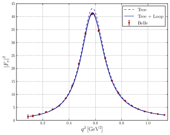
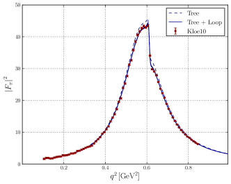
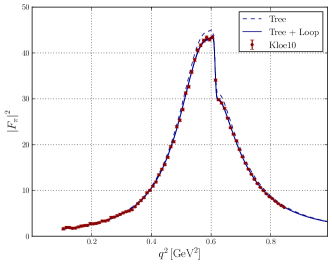
Figure 2: Fits to the pion form factor data extracted from $\tau$ decay Fujikawa:2008ma (left) and $e^{+}e^{-}$ scattering Ambrosino:2010bv (right). The systematic and statistical errors were added in quadrature for the $\tau$ decay data. In the first (second) row the $\omega$ mass is fixed (floating).

VI Conclusions

We have calculated the vector form factor of the pion in the framework of chiral EFT with vector mesons included as dynamical degrees of freedom. To renormalize the loop diagrams, we applied the CMS. Within this renormalization scheme, the given EFT has a consistent power counting. By fitting the available parameters of the Lagrangian, a satisfactory description of the data extracted from $\tau^{-}\rightarrow\nu_{\tau}\pi^{-}\pi^{0}$ decay has been obtained. On the other hand, to achieve a reasonable accuracy in describing the form factor extracted from $e^{+}e^{-}\to\pi^{+}\pi^{-}$ data, it is necessary to incorporate the $\rho^{0}$-$\omega$-$\gamma$ mixing. We included this mixing only at the tree level. While a satisfactory fit to the data has been obtained by fitting the mixing parameters, more work needs to be done to incorporate the isospin-symmetry-breaking effects in a systematic fashion. This is subject of a future project. From our results we conclude that a chiral EFT with explicitly incorporated resonance states is a promising candidate for a successful phenomenological description of data beyond the low-energy region of ChPT.

VII Appendix

The loop functions $A_{0}$, $B_{0}$, and $C_{0}$ contributing to the pion form factor diagrams are defined as follows:

$$A_{0}(m^{2}) =\frac{(2\pi)^{4-n}}{i\,\pi^{2}}\,\int\frac{d^{n}k}{k^{2}-m^{2}+i0^{+}}\,,$$

$$B_{0}(p^{2},m_{1}^{2},m_{2}^{2}) =\frac{(2\pi)^{4-n}}{i\,\pi^{2}}\,\int\frac{d^{n}k}{\left[k^{2}-m_{1}^{2}+i0^{+}\right]\left[(p+k)^{2}-m_{2}^{2}+i0^{+}\right]}\,,$$

$$C_{0}(p_{1}^{2},(p_{2}-p_{1})^{2},p_{2}^{2},m_{1}^{2},m_{2}^{2},m_{3}^{2})$$

$$=\frac{(2\pi)^{4-n}}{i\,\pi^{2}}\int\frac{d^{n}k}{\left[k^{2}-m_{1}^{2}+i0^{+}\right]\left[(p_{1}+k)^{2}-m_{2}^{2}+i0^{+}\right]\left[(p_{2}+k)^{2}-m_{3}^{2}+i0^{+}\right]}\,,$$

where $n$ is the space-time dimension.

To one-loop order, the wave function renormalization constant of the pion, $1+\delta Z_{\pi}$, is given by

$$\delta Z_{\pi} =\frac{1}{96F_{\pi}^{4}g^{2}\pi^{2}}\Biggl{(}\frac{3(M_{R}^{2}+c_{x}M_{\pi}^{2})^{2}}{M_{R}^{2}M_{\pi}^{2}}\biggl{\{}M_{R}^{2}[-M_{\pi}^{2}+A_{0}(M_{\pi}^{2})+(M_{R}^{2}-M_{\pi}^{2})B_{0}(M_{\pi}^{2},M_{R}^{2},M_{\pi}^{2})]$$

$$\quad-(M_{R}^{2}-3M_{\pi}^{2})A_{0}(M_{R}^{2})\biggr{\}}+[3(M_{R}^{2}+c_{x}M_{\pi}^{2})-4F_{\pi}^{2}g^{2}]A_{0}(M_{\pi}^{2})\Biggr{)}.$$ (17)

The contributions of the loop diagrams to the form factor read

$$D_{l1} =\frac{5(8F_{\pi}^{2}g^{2}-7M_{R}^{2})A_{0}(M_{\pi}^{2})}{384F_{\pi}^{4}g^{2}\pi^{2}}\,,$$

$$D_{l2+l3} =\frac{3M_{R}^{4}[A_{0}(M_{\pi}^{2})-A_{0}(M_{R}^{2})+(M_{R}^{2}-4M_{\pi}^{2})B_{0}(M_{\pi}^{2},M_{R}^{2},M_{\pi}^{2})]}{128F_{\pi}^{4}g^{2}M_{\pi}^{2}\pi^{2}}\,,$$

$$D_{l4} =-\frac{M_{R}^{6}}{128F_{\pi}^{6}g^{4}M_{\pi}^{2}\pi^{2}(M_{R}^{2}-q^{2})(q^{2}-4M_{\pi}^{2})}\Biggl{(}M_{R}^{2}\Biggl{\{}(M_{R}^{2}-4M_{\pi}^{2}+2q^{2})M_{\pi}^{2}$$

$$\quad\times[2B_{0}(q^{2},M_{\pi}^{2},M_{\pi}^{2})+(2M_{R}^{2}-4M_{\pi}^{2}+q^{2})C_{0}(M_{\pi}^{2},M_{\pi}^{2},q^{2},M_{\pi}^{2},M_{R}^{2},M_{\pi}^{2})]$$

$$\quad+(4M_{\pi}^{2}-q^{2})[A_{0}(M_{R}^{2})-A_{0}(M_{\pi}^{2})]+[16M_{\pi}^{4}-6q^{2}M_{\pi}^{2}+M_{R}^{2}(q^{2}-6M_{\pi}^{2})]$$

$$\quad\times B_{0}(M_{\pi}^{2},M_{R}^{2},M_{\pi}^{2})\Biggr{\}}+(M_{\pi}^{2}q^{2}-4M_{\pi}^{4})A_{0}(M_{R}^{2})\Biggr{)},$$

$$D_{l5} =\frac{M_{R}^{2}}{2304F_{\pi}^{4}g^{2}M_{\pi}^{2}\pi^{2}(M_{R}^{2}-q^{2})(q^{2}-4M_{\pi}^{2})}\,\Biggl{[}18M_{R}^{4}(4M_{\pi}^{2}-q^{2})A_{0}(M_{\pi}^{2})$$

$$\quad+18M_{R}^{4}[-16M_{\pi}^{4}+(8M_{R}^{2}+6q^{2})M_{\pi}^{2}-M_{R}^{2}q^{2}]B_{0}(M_{\pi}^{2},M_{\pi}^{2},M_{R}^{2})$$

$$\quad-18M_{\pi}^{2}M_{R}^{4}(-2M_{R}^{2}+8M_{\pi}^{2}-q^{2})(2M_{R}^{2}+q^{2})C_{0}(M_{\pi}^{2},M_{\pi}^{2},q^{2},M_{R}^{2},M_{\pi}^{2},M_{R}^{2})$$

$$\quad-2M_{\pi}^{2}(4M_{\pi}^{2}-q^{2})(12M_{R}^{4}-8q^{2}M_{R}^{2}+(q^{2})^{2})$$

$$\quad+6(4M_{\pi}^{2}-q^{2})[M_{\pi}^{2}(10M_{R}^{2}+q^{2})-3M_{R}^{4}]A_{0}(M_{R}^{2})$$

$$\quad-3M_{\pi}^{2}[24M_{R}^{6}+28q^{2}M_{R}^{4}-18(q^{2})^{2}M_{R}^{2}-(q^{2})^{3}+M_{\pi}^{2}(-64M_{R}^{4}+72q^{2}M_{R}^{2}+4(q^{2})^{2})]$$

$$\quad\times B_{0}(q^{2},M_{R}^{2},M_{R}^{2})\Biggr{]},$$

$$D_{l6} =\frac{5M_{R}^{4}A_{0}(M_{\pi}^{2})}{384F_{\pi}^{4}g^{2}\pi^{2}(M_{R}^{2}-q^{2})},$$

$$D_{l7} =\frac{M_{R}^{4}(3M_{R}^{2}-4F_{\pi}^{2}g^{2})[12M_{\pi}^{2}-2q^{2}+6A_{0}(M_{\pi}^{2})+3(4M_{\pi}^{2}-q^{2})B_{0}(q^{2},M_{\pi}^{2},M_{\pi}^{2})]}{2304F_{\pi}^{6}g^{4}\pi^{2}(M_{R}^{2}-q^{2})}\,,$$

$$D_{l8} =\frac{M_{R}^{4}A_{0}(M_{\pi}^{2})}{32F_{\pi}^{4}g^{2}\pi^{2}(M_{R}^{2}-q^{2})}\,,$$

$$D_{l9} =-\frac{3M_{R}^{4}[5M_{R}^{2}-6A_{0}(M_{R}^{2})]}{128F_{\pi}^{2}\pi^{2}(M_{R}^{2}-q^{2})^{2}}\,,$$

$$D_{l10} =\frac{M_{R}^{8}[2(q^{2}-6M_{\pi}^{2})-6A_{0}(M_{\pi}^{2})+3(q^{2}-4M_{\pi}^{2})B_{0}(q^{2},M_{\pi}^{2},M_{\pi}^{2})]}{1152F_{\pi}^{6}g^{4}\pi^{2}(M_{R}^{2}-q^{2})^{2}}\,,$$

$$D_{l11} =-\frac{1}{1152F_{\pi}^{2}\pi^{2}(M_{R}^{2}-q^{2})^{2}}\Biggl{[}9M_{R}^{6}-48q^{2}M_{R}^{4}+20(q^{2})^{2}M_{R}^{2}-2(q^{2})^{3}$$

$$\quad+6(3M_{R}^{4}+8q^{2}M_{R}^{2}+(q^{2})^{2})A_{0}(M_{R}^{2})$$

$$\quad+3(48M_{R}^{6}+68q^{2}M_{R}^{4}-16(q^{2})^{2}M_{R}^{2}-(q^{2})^{3})B_{0}(q^{2},M_{R}^{2},M_{R}^{2})\Biggr{]}.$$ (18)

References

• (1) S. Weinberg, Physica A 96, 327 (1979).
• (2) J. Gasser and H. Leutwyler, Ann. Phys. (N.Y.) 158, 142 (1984).
• (3) V. Bernard, Prog. Part. Nucl. Phys.  60, 82 (2008).
• (4) S. Scherer, Prog. Part. Nucl. Phys.  64, 1 (2010).
• (5) E. E. Jenkins, A. V. Manohar, and M. B. Wise, Phys. Rev. Lett.  75, 2272 (1995).
• (6) J. Bijnens and P. Gosdzinsky, Phys. Lett.  B 388, 203 (1996).
• (7) J. Bijnens, P. Gosdzinsky, and P. Talavera, Nucl. Phys.  B501, 495 (1997).
• (8) J. Bijnens, P. Gosdzinsky, and P. Talavera, JHEP 9801, 014 (1998).
• (9) J. Bijnens, P. Gosdzinsky, and P. Talavera, Phys. Lett.  B 429, 111 (1998).
• (10) R. G. Stuart, in ${\rm Z}^{0}$ Physics, ed. J. Tran Thanh Van (Editions Frontieres, Gif-sur-Yvette, 1990), p.41.
• (11) A. Denner, S. Dittmaier, M. Roth, and D. Wackeroth, Nucl. Phys.  B560, 33 (1999).
• (12) A. Denner and S. Dittmaier, Nucl. Phys. Proc. Suppl.  160, 22 (2006).
• (13) A. Denner, S. Dittmaier, M. Roth, and L. H. Wieders, Nucl. Phys.  B724, 247 (2005).
• (14) S. Actis and G. Passarino, Nucl. Phys.  B777, 100 (2007).
• (15) S. Actis, G. Passarino, C. Sturm, and S. Uccirati, Phys. Lett.  B 669, 62 (2008).
• (16) A. Denner and J. N. Lang, arXiv:1406.6280 [hep-ph].
• (17) D. Djukanovic, J. Gegelia, A. Keller, and S. Scherer, Phys. Lett.  B 680, 235 (2009).
• (18) D. Djukanovic, J. Gegelia, and S. Scherer, Phys. Lett.  B 690, 123 (2010).
• (19) T. Bauer, J. Gegelia, and S. Scherer, Phys. Lett. B 715, 234 (2012).
• (20) D. Djukanovic, E. Epelbaum, J. Gegelia, and U.-G. Meißner, Phys. Lett. B 730, 115 (2014).
• (21) T. Bauer, S. Scherer, and L. Tiator, Phys. Rev. C 90, 015201 (2014).
• (22) I. Rosell, J. J. Sanz-Cillero, and A. Pich, JHEP 0408, 042 (2004).
• (23) P. C. Bruns and U.-G. Meißner, Eur. Phys. J.  C 40, 97 (2005).
• (24) P. C. Bruns and U.-G. Meißner, Eur. Phys. J.  C 58, 407 (2008).
• (25) S. Leupold, Phys. Rev.  D 80, 114012 (2009).
• (26) C. Terschlüsen and S. Leupold, Phys. Lett.  B 691, 191 (2010).
• (27) Y. Nambu, Phys. Rev.  106, 1366 (1957).
• (28) W. R. Frazer and J. R. Fulco, Phys. Rev. Lett.  2, 365 (1959).
• (29) M. Gell-Mann and F. Zachariasen, Phys. Rev.  124, 953 (1961).
• (30) J. J. Sakurai, Currents and Mesons (University of Chicago Press, Chicago, 1969), Chap. 3.
• (31) R. P. Feynman, Photon-Hadron Interactions (Benjamin, Reading, Massachusetts, 1972), Chaps. 14-21.
• (32) S. Actis et al. [Working Group on Radiative Corrections and Monte Carlo Generators for Low Energies Collaboration], Eur. Phys. J. C 66, 585 (2010).
• (33) B. B. Brandt, A. Jüttner, and H. Wittig, JHEP 1311, 034 (2013).
• (34) C. Hanhart, Phys. Lett. B 715, 170 (2012).
• (35) G. Ecker, J. Gasser, H. Leutwyler, A. Pich, and E. de Rafael, Phys. Lett.  B 223, 425 (1989).
• (36) D. Djukanovic, M. R. Schindler, J. Gegelia, G. Japaridze, and S. Scherer, Phys. Rev. Lett.  93, 122002 (2004).
• (37) K. Kawarabayashi and M. Suzuki, Phys. Rev. Lett.  16, 255 (1966).
• (38) Riazuddin and Fayyazuddin, Phys. Rev.  147, 1071 (1966).
• (39) F. Jegerlehner and R. Szafron, Eur. Phys. J. C 71, 1632 (2011).
• (40) M. Fujikawa et al. [Belle Collaboration], Phys. Rev. D 78, 072006 (2008).
• (41) F. Ambrosino et al. [KLOE Collaboration], Phys. Lett. B 700, 102 (2011).
• (42) D. Djukanovic, M. R. Schindler, J. Gegelia, and S. Scherer, Phys. Rev. Lett.  95, 012001 (2005).
• (43) J. J. Sanz-Cillero and A. Pich, Eur. Phys. J. C 27, 587 (2003).