Budding of domains in mixed bilayer membranes

Abstract

We propose a model that accounts for budding behavior of domains in lipid bilayers, where each of the bilayer leaflets has a coupling between its local curvature and local lipid composition. The compositional asymmetry between the two monolayers leads to an overall spontaneous curvature. The membrane free-energy contains three contributions: bending energy, line tension, and a Landau free-energy for a lateral phase separation. Within a mean-field treatment, we obtain various phase diagrams which contain fully-budded, dimpled and flat states. In particular, for some range of membrane parameters, the phase diagrams exhibit a tricritical behavior as well as three-phase coexistence region. The global phase diagrams can be divided into three types and are analyzed in terms of the curvature-composition coupling parameter and domain size.

I Introduction

Biological membranes are multi-component assemblies typically composed of lipids, cholesterol, glyco-sugars, and proteins, whose presence is indispensable to the normal functioning of living cells AlbertsBook . Given the complexity of biological membranes, studies of model membranes have been conducted in vitro in order to gain insight on the structural and physical behavior of biomembranes. Many studies, in particular over the last two decades, have focused on simplified artificial systems containing vesicles in solution, composed of ternary mixtures of lipids and cholesterol VK05 ; SK_DA_Review . By decreasing temperature, the ternary mixtures undergo a phase separation between a liquid-ordered (L_o) phase and a liquid-disordered (L_d) one VK ; YIMKO . Depending on thermodynamical parameters, the liquid domains show one of three distinct domain shapes: flat, dimpled (partially budded), or fully-budded UrsellBook .

A theoretical model for domain-induced budding of planar membranes was proposed by Lipowsky Lipowsky92 ; Lipowsky93 , and later was extended for the case of closed vesicles JL93 ; JL96 . In the model, the competition between membrane bending-energy and domain line-tension leads to a budding transition under the constraint of fixed domain area. Hu et al. hu proposed a mechanism based on this interplay, which stabilizes patterns of several domains on closed vesicles without requiring any osmotically induced membrane tension.

Returning to the case of planar membranes, Lipowsky’s model Lipowsky14 predicts that: (i) an initially flat domain deforms spontaneously into a completely spherical bud when the initial domain size exceeds a critical size; and (ii) dimpled domains are stable only when the spontaneous curvature of the bilayer membrane is nonzero. The latter prediction was later re-examined UKP , because dimpled domains are observed experimentally in vesicles with no apparent spontaneous curvature baumgart . In order to resolve this discrepancy, Rim et al. RUPK considered the effect of adding an overall lateral tension acting on the membrane, and used ideas about entropy-driven lateral tension that were originally proposed by Helfrich and Servuss HS . The resulting phase diagram RUPK contains regions of stability for the three different domain morphologies as mentioned above. Moreover, the effect of the lateral tension on budding was discussed by Lipowsky and coworkers Lipowsky92 ; lischi . In particular, the budding process requires that the activation energy has to exceed the energy barrier associated with the surface tension.

In this paper, we propose a model that describes domain-induced budding in bilayers composed of a binary mixture of lipids. We suggest that dimpled domains can be formed and remain stable due to a possible asymmetry between the two monolayer compositions. We show that the dimpled structure appears when the line tension along the domain rim is not too large. Global phase diagrams are calculated within mean-field theory and, in some range of system parameters, we obtain a tricritical behavior as well as three-phase coexistence region. We discuss different morphologies that characterize the phase diagrams in terms of model parameters.

It has been recognized long time ago that such an asymmetry in monolayer composition leads to a nonzero bilayer spontaneous curvature SPA ; SPAM . The coupling between composition and monolayer curvature was also considered MS in order to describe the transition between lamellar and vesicular phases of bilayer membranes composed of two types of amphiphiles. It is worthwhile mentioning related works by Harden et al. HM94 ; harden and Góźdź et al. GG01 , who studied budding and domain shape transformations in bilayer membranes. In Refs. HM94 ; harden , the phase separation is assumed to occur only in one of the monolayers, and the domain spontaneous curvature due to the compositional asymmetry is kept constant. For finite spontaneous curvatures, it was shown that the dimpled domains are obtained in equilibrium when both line and surface tensions are small harden . More recently, ring-shaped domains were experimentally obtained in model membranes by using a bud-mimicking topography Ryu . Such a ring-shaped domain is located around a bud-neck region having a negative curvature, and is characterized by the composition asymmetry between the two monolayers.

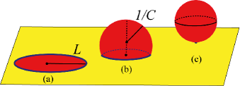
Figure 1: (a) The flat phase, (b) the dimpled phase, and (c) the fully-budded phase. In (a) the circular flat domain (red) has a radius $L$ and area $S=\pi L^{2}$. In (b) a bud of the same area $S$ forms a spherical cap of radius $1/C$, where $C$ is the curvature, embedded in an otherwise flat membrane. In (c) a fully-budded domain of area $S$ has a spherical shape, just touching the flat membrane. The line tension $\gamma$ acts along the boundary (blue line) between the domain and the flat membrane.

The outline of our paper is as follow. In the next section, we present a model for bilayer domains. In Sec. III, various mean-field phase diagrams are obtained by changing the ratio between the domain size and the invagination length, as well as tuning the inter-monolayer coupling parameter strength. Finally, Sec. IV includes some discussion and interpretation of our results.

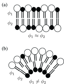
Figure 2: (a) Flat bilayer domain when the relative A/B compositions in the two monolayers, $\phi_{1}$ and $\phi_{2}$, are almost symmetric, $\phi_{1}\approx\phi_{2}$. (b) Curved bilayer domain when the compositions are asymmetric, $\phi_{1}\neq\phi_{2}$. The spontaneous curvature of each monolayer is assumed to depend linearly on the composition, as given by Eq. (4).

II Model

We model the membrane as a bilayer having two monolayers (leaflets), each composed of an A/B mixture of lipids that can partition themselves asymmetrically between the two monolayers. We consider the case where the lipids can undergo a lateral phase separation creating domains rich in one of the two components. As discussed below, these domains can also deform (bud) in the normal direction, and the deformations are controlled by the membrane curvature elasticity. Because we do not include any gradient terms in the free energy, it results in an unrealistic discontinuous jump of the membrane curvature close to the bud edge. For the fully-budded state this jump in curvature does not matter because the bud neck corresponds to a small length scale of the order of the membrane thickness. However, in the dimpled state, this jump occurs on a bigger length scales and artificially affects the free energy. We will further introduce a coupling between local lipid composition and local curvature SPA ; SPAM ; MS , which can eventually drive the budding process of the membrane.

We start by considering a single two-dimensional (2D) circular domain of an initial and arbitrary radius $L$ embedded in an otherwise flat (2D) membrane, as shown in Fig. 1(a). The area of the domain, $S=\pi L^{2}$, is assumed to stay constant even when the domain buds into the third dimension. For simplicity, we consider only budded domains whose shape is a spherical cap of radius $1/C$ (Fig. 1(b)). The total bending energy of the budded domain is given by adding the curvature contributions from the two monolayers Helfrich73 ; SafranBook :

$$E_{\rm b}=2\pi L^{2}\kappa\left[(C-C_{0})^{2}+(C+C_{0})^{2}\right],$$ (1)

where $\kappa$ is the bending rigidity modulus and $C_{0}$ the monolayer spontaneous curvature. As shown in Fig. 2, the two monolayers are fully coupled together, and their curvatures are given by $+C$ and $-C$, respectively.

The next contribution is the domain edge energy that is proportional to the edge length and its line tension, $\gamma$ Lipowsky92 :

$$E_{\rm ed}=2\pi L\gamma\sqrt{1-(LC/2)^{2}}.$$ (2)

In the extreme case, when the domain buds into a complete spherical domain as in Fig. 1(c), $C=\pm 2/L$ and $E_{\rm ed}=0$.

For domains that are composed of two different lipid types, the relative composition in each monolayer is defined as $\phi_{i}=\phi_{i}^{\rm A}-\phi_{i}^{\rm B}$ ($i=1,2$), where $\phi_{i}^{\rm A}$ ($\phi_{i}^{\rm B}$) is the molar fraction of the ${\rm A}$ lipid ($\rm B$ lipid) in the $i$-th monolayer. We assume that each of the monolayers is incompressible, hence, $\phi_{i}^{\rm A}$+$\phi_{i}^{\rm B}=1$. For simplicity sake, the molecular areas of A and B species are taken to be the same, meaning that the molar fraction of the lipids is indenting to their area fraction. As in any A/B mixture, the possibility of a phase separation due to partial incompatibility between the two species can be described by a phenomenological Landau expansion of the free energy in powers of $\phi_{i}$ around the critical point, $\phi_{i}=0$. In our case, this expansion is done separately for each monolayer, and the free energy is the sum of the two contributions:

$$E_{\rm ph}=\pi L^{2}\frac{U}{\Xi^{2}}\sum_{i=1}^{2}\left[\frac{t}{2}\phi_{i}^{2}+\frac{1}{4}\phi_{i}^{4}-\mu\phi_{i}\right],$$ (3)

where $\Xi\equiv\kappa/\gamma$ is the invagination length, $U$ a parameter that sets the energy scale, $t\sim(T-T_{\rm c})/T_{\rm c}$ the reduced temperature ($T_{\rm c}$ being the critical temperature), and $\mu$ the chemical potential that fixes the A/B relative composition in each layer. In general, a different chemical potential can be assigned to each of the two monolayers. However, since it is difficult to control the average composition in each layer separately, we introduce only one chemical potential $\mu$ that fixes the total relative composition $\phi_{1}+\phi_{2}$ of the entire bilayer. Notice that we allow exchange of lipid molecules between the two monolayers via a flip-flop process. Bilayers where each of the monolayer compositions can be controlled independently will be addressed in our future work.

As argued before MS , we do not include any $\phi_{i}$ gradient term in Eq. (3) because we consider only homogeneous composition within a single domain. The energy cost associated with a gradient term in composition is effectively taken into account through the line tension $\gamma$ in Eq. (2), which is regarded here as an external control parameter. This assumption of $\gamma$ can be justified for situations of strong segregation (far from the critical point) between the domain and the background, for which the domain boundary is sharp.

Hereafter, we will use several dimensionless variables: a rescaled curvature $c\equiv LC$, rescaled spontaneous curvature $c_{0}\equiv LC_{0}$, and rescaled invagination length $\xi\equiv\Xi/L$. The coupling between the spontaneous curvature $c_{0}$ and composition is taken into account by assuming a linear dependence on $\phi_{i}$ MS (see also Fig. 2):

$$c_{0}(\phi_{i})=\bar{c}_{0}-\beta\phi_{i},$$ (4)

where all variables in Eq. (4) are dimensionless, $\bar{c}_{0}$ is the spontaneous curvature of the monolayer at its critical composition $\phi_{i}=0$, and $\beta$ a coupling constant. Since $\bar{c}_{0}$ is a constant that merely shifts the origin of the chemical potential $\mu$, we can drop it without loss of generality.

The total free-energy of the bilayer model is given by the sum of Eqs. (1), (2), and (3):

$$E_{\rm tot}=E_{\rm b}+E_{\rm ed}+E_{\rm ph}.$$ (5)

Denoting the average and difference of the two monolayer compositions, respectively, by

$$\phi_{+}\equiv\frac{\phi_{2}+\phi_{1}}{2}~{}~{}~{}{\rm and}~{}~{}~{}\phi_{-}\equiv\frac{\phi_{2}-\phi_{1}}{2},$$ (6)

the dimensionless total free-energy of one domain, $\varepsilon=E_{\rm tot}/2\pi\kappa$, is expressed as

$$\varepsilon =2c^{2}-4\beta c\phi_{-}+2\beta^{2}(\phi_{+}^{2}+\phi_{-}^{2})$$

$$+\frac{1}{\xi}\sqrt{1-c^{2}/4}$$

$$+\frac{1}{\xi^{2}}\left(\frac{U}{2\kappa}\right)\biggl{[}t(\phi_{+}^{2}+\phi_{-}^{2})$$

$$+\frac{1}{2}(\phi_{+}^{4}+6\phi_{+}^{2}\phi_{-}^{2}+\phi_{-}^{4})-2\mu\phi_{+}\biggr{]},$$ (7)

where we have dropped unimportant constant terms. Within a mean-field theory, the equilibrium state of the system and the phase transitions are determined by minimization of the above $\varepsilon$ with respect to $\phi_{\pm}$ and $c$.

We note that Eq. (7) depends on three dimensionless parameters: $\beta$, $\xi$, and $U/2\kappa$, while the thermodynamic variables are the temperature $t$, and the three order parameters: $\phi_{\pm}$ and $c$. In the calculations presented hereafter, we set $U/(2\kappa)=1$ and vary the values of $\beta$ and $\xi$. Since the total free energy is invariant under simultaneous exchange of $\beta\rightarrow-\beta$ and $\phi_{-}\rightarrow-\phi_{-}$, it is sufficient to study only the $\beta>0$ range.

Typical experimental values of flat domain size are in the range of $L\simeq 50$ – $500$ nm SI , the bending rigidity $\kappa\simeq 10^{-19}$ J $\approx 25k_{\rm{}_{B}}T$ SafranBook , and line tension in the range of $\gamma\simeq 0.2$ – $6.2\times 10^{-12}$ J/m baumgart ; tian . These parameter values yield invagination length, $\Xi$, of the order $0.01L$ to $10L$ ($\xi\simeq 0.01$ – $10$), as will be used in the next section.

III Phase Behavior and Phase Diagrams

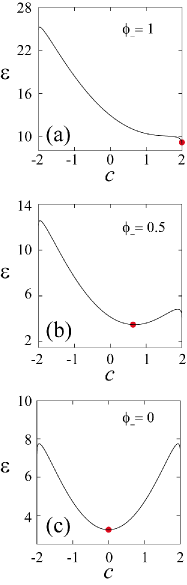
Figure 3: Plots of the free energy $\varepsilon$ as a function of the curvature $c$ for (a) $\phi_{-}=1$, (b) $\phi_{-}=0.5$, and (c) $\phi_{-}=0$. The other parameter values are: $t=-0.5$, $\phi_{+}=0.4$, $\beta=1$, and $\xi=0.25$. The free-energy minimum is shown by a red dot, and corresponds to the fully-budded state ($c=2$), dimpled state ($0<c<2$), and flat state ($c=0$), in (a), (b) and (c), respectively.

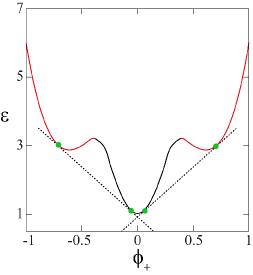
Figure 4: Plot of the free energy $\varepsilon$ as a function of $\phi_{+}$ for $t=-0.5$, $\beta=1$, and $\xi=0.25$. The red and black lines of the free energy correspond to the flat and fully-budded states, respectively. The two dashes lines are the common tangent constructions, which determine two sets of coexisting compositions indicated by green dots.

III.1 Flat, dimpled and fully-budded states

The total free energy $\varepsilon$ in Eq. (7) is first minimized with respect to the curvature $c$, yielding

$$4c-4\beta\phi_{-}-\frac{c}{4\xi\sqrt{1-c^{2}/4}}=0.$$ (8)

The above equation indicates that the value of $c$, taken at the minimum of $\varepsilon$, uniquely determines the value of $\phi_{-}$, as long as $|c|<2$. The value of the curvature determines which of the domain states is the equilibrium one: flat (F) with $c=0$, fully-budded (B) with $c=\pm 2$, or dimpled (D) with $0<|c|<2$. By substituting back the above minimization condition for $|c|<2$ into the total free energy, we obtain $\varepsilon(\phi_{+},\phi_{-})$ as a function of $\phi_{+}$ and $\phi_{-}$. This free energy is further minimized with respect to $\phi_{-}$, leading to an expression $\varepsilon(\phi_{+})$ that is only a function of $\phi_{+}$. We assume that the average composition $\phi_{+}$ is a conserved order-parameter (while $c$ and $\phi_{-}$ are non-conserved), and can be controlled by varying the conjugate chemical potential $\mu$ acting as a Lagrange multiplier.

In order to illustrate this minimization process, we plot $\varepsilon$ as a function of the curvature $c$ in Fig. 3, for given values of $t$ and $\phi_{\pm}$. We see that the free energy takes its minimum at different curvature values (marked by red circles) for different $\phi_{-}$ values. Figure 3(a), (b) and (c) correspond to the fully-budded, dimpled and flat states, respectively. In Figure 4 the free energy $\varepsilon$ that was minimized with respect to both $c$ and $\phi_{-}$ is plotted as a function of $\phi_{+}$ for a fixed temperature. Different colors of the free energy plot correspond to different domain states (F and B). The two dashes lines are the common tangents that determine the two sets of coexisting compositions. For the chosen parameter values as in Fig. 4, the flat and fully-budded phases are in coexistence (F+B and B+F).

III.2 Phase diagrams

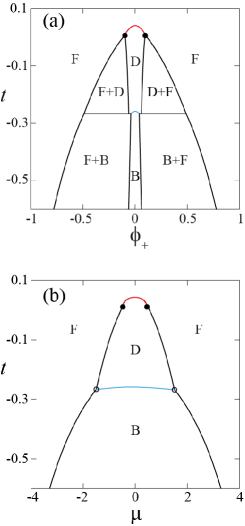
Figure 5: (a) Phase diagram in the ($\phi_{+}$, $t$) plane, where $\phi_{+}$ is the average composition and $t$ the reduced temperature; and, (b) in the ($\mu$, $t$) plane, where $\mu$ is the chemical potential. The parameters are $\beta=1$ and $\xi=0.25$. “F”, “D”, and “B” stand, respectively, for flat, dimpled, and fully-budded phases. Coexistence regions are denoted by “F+D” etc. in (a). The black and red lines indicate first- and second-order phase transitions, respectively, while the blue line indicates a first-order phase transition with a discontinuous jump in both $c$ and $\phi_{-}$. The filled circles represent the tricritical points ($t_{\rm tcp}\simeq 0.011$, $\phi_{+}^{\rm tcp}\simeq\pm 0.094$, $\mu_{\rm tcp}\simeq\pm 0.488$), and the open circles in (b) represent the triple points ($t_{\rm tri}\simeq-0.267$, $\mu_{\rm tri}\simeq\pm 1.49$), where three phases coexist, with $\phi_{+}^{\rm tri}=\pm 0.484,\pm 0.066$, and $\pm 0.045$.

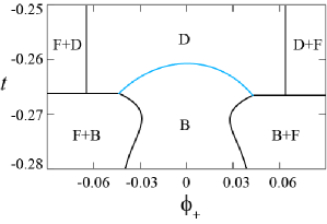
Figure 6: Enlarged middle-zone ($\phi_{+}\approx 0$ and $t$ around the triple point value) of Fig. 5(a). The blue line is a first-order phase transition between dimpled and fully-budded phases, with a jump in the curvature value from $c\simeq 0.75$ to $c=2$. The solid black lines indicate the boundaries of the two-phase coexistence regions: F+D and F+B. On the triple line, $t_{\rm tri}\simeq-0.267$, three phases coexist with $\phi_{+}^{\rm tri}=\pm 0.066$ and $\pm 0.045$.

The numerically-computed phase diagrams are three-dimensional ones for fixed values of $\xi$ and $\beta$. They can be plotted either in the $(\phi_{+},t,c)$ or $(\mu,t,c)$ parameter space. We recall that the throughout this work we set for simplicity, $U/(2\kappa)=1$. In addition, note that the equilibrium $\phi_{-}$ value is self-determined by the equilibrium $c$ value according to Eq. (8). As it is too cumbersome to present 3D plots, we plot 2D phase diagrams in the $(\phi_{+},t)$ or $(\mu,t)$ planes, which represent a projection in the $c$ direction, or 2D cuts in the $(c,t)$ plane for fixed values of the conserved order-parameter, $\phi_{+}$ (see Fig. 8).

In Fig. 5 we present the phase diagrams that are obtained numerically for $\beta=1$ and $\xi=0.25$. In (a) the phase diagram is plotted in the $(\phi_{+},t)$ plane, and in (b) in the $(\mu,t)$ plane. The phase diagram in (a) is symmetric about $\phi_{+}=0$, and in (b) about $\mu=0$. At high temperatures only the flat phase is stable. For lower temperatures, in the range $-0.267<t<0.042$, the dimpled phase becomes stable. The phase diagrams show a tricritical behavior, similar to the well-known tricritical behavior of Blume–Emery–Griffiths spin–one model BEG .

The red line in Fig. 5 denotes a second-order phase transition between F and D phases, occurring when $c\rightarrow 0$. It terminates at two symmetric tricritical points (filled circles), $t_{\rm tcp}\simeq 0.011$, $\phi_{+}^{\rm tcp}\simeq\pm 0.094$ in (a), and $\mu_{\rm tcp}\simeq\pm 0.488$ in (b). The tricritical points are also obtained analytically using some approximations and their calculated values, $t_{\rm tcp}\simeq 0.014$ and $\phi_{+}^{\rm tcp}\simeq\pm 0.095$, agree well with the numerical ones. More details on the analytical derivations are provided in the Appendix. For $t<t_{\rm tcp}$, the phase transition between F and D becomes first-order (solid black line) with coexistence lines in the $(\mu,t)$ plane and two coexistence regions, marked as F+D and D+F in the $(\phi_{+},t)$ plane. As one crosses this phase transition line, there is a jump in $\phi_{+}$, as well as in $c$ and $\phi_{-}$, and the jump in $\phi_{-}$ is fully determined by a similar jump in $c$.

Two triple points are shown as open circles in Fig. 5(b) at $t_{\rm tri}\simeq-0.267$ and $\mu_{\rm tri}\simeq\pm 1.49$, or equivalently as a horizontal line in Fig. 5(a). At the triple point, the three phases (F, D and B) coexist. In order to explain in more detail the phase behavior close to the triple line, we show in Fig. 6 an enlarged section of Fig. 5(a) around the triple line. The tip of the middle (blue) line starts at about $t\simeq-0.261$ and terminates at the triple-point temperature. This is a first-order phase transition line where both $c$ and $\phi_{-}$ have a discontinuous jump from their dimpled values ($c\simeq 0.75$) to their fully-budded values ($c=2$). The other solid lines delimit the two-phase coexistence regions: F+D above the triple line and F$+$B below it.

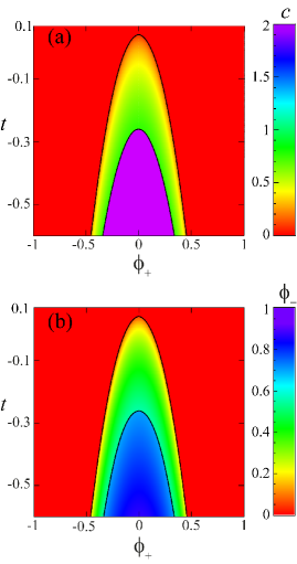
Figure 7: (a) The curvature $c$ as a contour plot in the ($\phi_{+}$, $t$) plane, with a color bar that corresponds to $0\leq c\leq 2$. A jump from $c=2$ to about $0.75$ can be seen as $t$ increases its value and eventually crosses the lower black line, while along the upper black line $c$ vanishes continuously. In (b) the compositional asymmetry between the two monolayers, $\phi_{-}$, is plotted as a contour plot in the ($\phi_{+}$, $t$) plane. As $t$ increases, a jump is seen from $\phi_{-}=0.7$ to $0.55$ along the lower black curve. For the upper black curve $\phi_{-}$ vanishes continuously (just as $c$ was). The chosen parameters are $\beta=1$ and $\xi=0.25$.

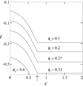
Figure 8: The reduced temperature $t$ as function of the equilibrium curvature $c$ for fixed values of $\beta=1$, $\xi=0.25$, and several values of $\phi_{+}=0.1,0.2,0.27,0.33$ and $0.4$. As $t$ decreases, the curvature $c$ first continuously increases from zero, and then discontinuously jumps from $c\simeq 0.75$ (marked by an arrow on the $c$-axis) to $c=2$. The former corresponds to the second-order phase transition from the flat state to the dimpled one, while the latter to the first-order phase transition from the dimpled state to the fully-budded one.

In Fig. 7(a), we plot the equilibrium values of $c$, and those of $\phi_{-}$ in (b), in order to view more clearly the phase transitions. Both $c$ and $\phi_{-}$ are plotted in the $(\phi_{+},t)$ plane as a contour color plot. In (a) we see two parabola-like lines delimiting different values of $c$. At the upper black line, the curvature continuously tends towards zero, $c\rightarrow 0$. The region close to the curve tip ($\phi_{+}\approx 0$) coincides with the second-order phase transition between F and D phases (the red line of Fig. 5(a)), while the rest of the line lies inside the two-phase coexistence region, and does not influence the equilibrium state of the system. The lower blue line represents a jump in $c$ from $c\simeq 0.75$ (D phase) to $c=2$ (B phase). Its top region (close to $\phi_{+}=0$) coincides with the first-order phase transition between D and B phases (the blue lines in Figs. 5(a) and 6), and the rest of the line lies within the F+B coexistence region. In Fig. 7(b), a similar contour plot is shown for $\phi_{-}$, as is determined by Eq. (8).

The complementary plot is shown in Fig. 8 in the $(c,t)$ plane for several fixed values of $\phi_{+}$ ranging from 0.1 to 0.4. We recall that $\phi_{+}=(\phi_{1}+\phi_{2})/2=(\phi^{\rm A}_{1}+\phi^{\rm A}_{2})/2-(\phi^{\rm B}_{1}+\phi^{\rm B}_{2})/2$ is a conserved quantity determined by the total amount of the A and B lipids in the domain. In the model we control it by the chemical potential $\mu$. As $t$ is lowered, the minimized curvature $c$ continuously increases from zero. This represent a continuous (second-order) phase transition from the flat state (F with $c=0$) to the dimpled one (D with $c>0$). When the temperature is lowered even further, the curvature discontinuously jumps from $c\simeq 0.75$ (indicated by an arrow on Fig. 8) to $c=2$. This is a first-order phase transition from the dimpled state (D) to the fully-budded (B) one. Notice that the maximum curvature $c\simeq 0.75$ of the dimpled state does not depend on the average composition $\phi_{+}$.

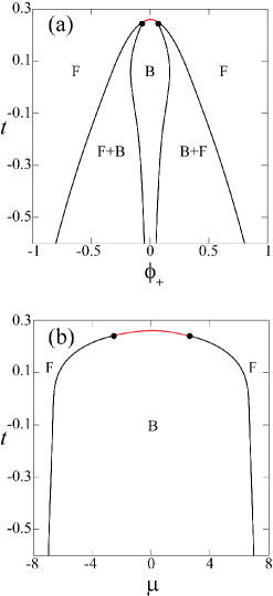
Figure 9: (a) Phase diagram in the ($\phi_{+}$, $t$) plane, and (b) in the ($\mu$, $t$) plane for $\beta=1$ and $\xi=1/7\simeq 0.143$. The meaning of the lines and symbols is the same as in Fig. 5. A critical (red) line separates the F and B phases and terminates at two tricritical points (filled circles) with $(t_{\rm tcp}\simeq 0.240,\phi_{+}^{\rm tcp}\simeq\pm 0.063,\mu_{\rm tcp}\simeq\pm 2.64)$. For $t<t_{\rm tcp}$, coexistence regions, B+F and F+B, separate the F and B phases.

When the $\xi$ value is decreased, while keeping $\beta$ fixed, the D phase disappears, and the only remaining stable phases are F and B, with a phase transition between them. This is shown on Fig. 9 where the chosen parameter values are $\beta=1$ and $\xi=1/7\simeq 0.143$. A second-order phase transition (red line) is seen between the F and B phases in the proximity of the symmetric $\phi_{+}=0$ axis. This second-order line ends at two tricritical points located at $t_{\rm tcp}\simeq 0.240$ and $\phi_{+}^{\rm tcp}\simeq\pm 0.063$ in (a), or equivalently, $\mu_{\rm tcp}\simeq\pm 2.64$ in (b). Below the tricritical temperature, the coexistence region is between the F and B phases (F+B), and is delimited by the solid black lines. Note that as the D phase disappeared there is no three-phase coexistence at these parameters values. The disappearance of the D phase can be understood in the following way. Smaller values of the invagination length, $\xi=\kappa/(L\gamma)$, correspond to larger values of the line tension $\gamma$, and domains will fully bud for lower temperatures without showing any D state.

At yet lower values of $\xi$, the line tension is large enough so that only the B phase exists, while the F phase disappears. In Fig. 10, we present such a phase diagram for $\beta=1$ and $\xi=0.125$. The only coexistence regions are between different fully-budded phases, denoted as B1+B2 and B2+B3. Each of these coexistence regions terminates at critical points (filled squares), $t_{\rm c}\simeq-0.028$, $\phi_{+}^{\rm c}\simeq\pm 0.251$ and $\mu_{\rm c}\simeq\pm 8$.

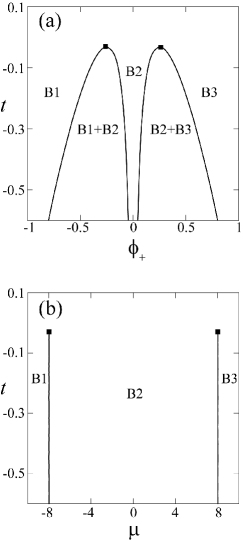
Figure 10: (a) Phase diagram in the ($\phi_{+}$, $t$) plane, and (b) in the ($\mu$, $t$) plane for $\beta=1$ and $\xi=0.125$. The meaning of the lines and symbols is the same as in Fig. 5. Only the B domain is stable and a first-order phase transition separates between B1 and B2, and another one between B2 and B3. Each of the coexistence regions terminates at a critical point $(t_{\rm c}\simeq-0.028,\phi_{+}^{\rm c}\simeq\pm 0.251,\mu_{\rm c}\simeq\pm 8)$. The filled squares correspond to the critical points.

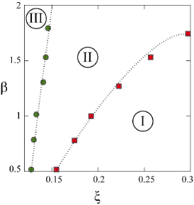
Figure 11: Behavior diagram as a function of $\xi=\Xi/L$ and the monolayer coupling parameter $\beta$. Examples of type I, II, III phase-diagram morphologies are given in Figs. 5, 9, and 10, respectively. The red squares delimit the calculated borderline between type I and II behavior, while the green circles delimit the calculated crossover between type II and III. The dashed lines serve only as a guideline to the eye and the error bar of the data points is about $\pm 0.1$ in $\beta$.

III.3 Effects of $\xi$ and $\beta$ on the phase behavior

By exploring the entire parameter range of $\xi$ and $\beta$, we find the crossover between the three types of phase diagrams as represented in Figs. 5 (type I), 9 (type II), and 10 (type III). This is shown in Fig. 11, where we present the stability regions for each of these three phase behaviors in the ($\xi$, $\beta$) plane. Type I is characterized by the existence of a dimpled phase, and has a triple point where the D, B and F phases coexist. In type II, the tricritical points exist but the triple points and the D phase disappear. Type III is dominated by various B phases, with coexistence regions between them that terminate at a critical point. The crossover line between type II and III behaviors is almost a straight line, while the crossover line from type II to I is almost linear for $\beta<1.25$, and then saturates at about $\beta\simeq 1.8$. This saturation occurs when the coupling is strong (large $\beta$) and/or the domain size is small (large $\xi$). At these values, budding is promoted because of the large spontaneous curvature.

When $\xi$ decreases, for a fixed value of the coupling parameter $\beta$, the B phase swells and the D phase disappears, signaling the crossover between type I and II. Upon further decrease of $\xi$, only the B phase stays, i.e., crossover between type II and III. On the other hand, the larger $\beta$ is, the larger is the spontaneous curvature that favors the fully-budded state. For this reason, at higher values of $\beta$, the system buds at lower temperatures for the same value of $\xi$.

IV Discussion

We have proposed a model that accounts for domain budding of lipid bilayers, where each of the bilayer leaflets has a coupling between its local curvature and local A/B lipid composition. The composition asymmetry between the two leaflets is equivalent to the introduction of a membrane spontaneous curvature. This spontaneous curvature is not taken to be fix (as was assumed in previous works), but is calculated and depends on the asymmetry in leaflet composition. Hence, due to this extra mechanism of generating a spontaneous curvature, dimpled domains can be stabilized even for bilayers with a nominal zero spontaneous curvature. Our free-energy model contains three contributions: bending energy accounting for domain deformation in the normal direction, line tension along the rim of the budded or flat domain, and a Landau free-energy expansion that accounts for a lateral phase separation of the binary lipid mixture. We assume that the domain area remains constant during the budding process.

Our model predicts three states for domain as were observed experimentally: fully-budded (B), dimpled (D) and flat (F) states. In particular, in some range of parameters, the D state is found to be the most stable one. The obtained results indicate that for a certain range of temperatures, monolayer composition, domain size and coupling between curvature and composition, a triple point can appear. At the triple point, the B, D and F phases coexist, each with its own composition. Such a triple point has been reported already by Harden et al. harden . Moreover, we also found a tricritical point that corresponds to the intersection of a critical (second-order) line, which joins a first-order phase transition region between F and D. Finally, three types of phase diagram morphologies are found and analyzed in terms of the coupling parameter $\beta$ and domain size $\xi$ (see Fig. 11).

Formation of domains in membranes and their understanding remain an open and ever-challenging problem, even after an intense research in the last two decades. Many hypotheses have been proposed to explain the domain appearance and their possible structure and function VK05 ; SK_DA_Review ; LS .

One of the important assumptions in our model is that the domain size $L$ and area $S$ remain fixed during the budding process. Domains of fixed size can be obtained in thermodynamical equilibrium for a binary mixed membrane that undergoes a lateral micro-phase separation, and forms a 2D modulated phase with an equilibrated spatial periodicity SA . This a micro-phase separation can be driven by a coupling between local lipid composition and membrane curvature, leading to a curvature instability leibler ; andel ; kawa ; taniguchi , as was in particular discussed in Refs. KK ; kumar . When the A/B average lipid composition is off-critical, circular domains rich in one of the lipid can form spontaneously and be arranged in a hexagonal array, embedded in a background rich in the second lipid. These circular domains are characterized by their equilibrium fixed size, and can undergo a budding process as explored in the present work.

Formation of finite-size domains in equilibrium can also be explained by the presence of hybrid lipids having one saturated tail and a second unsaturated one BPS09 . Such hybrid lipids decrease the domain line tension YBS ; PS13 ; PS14 and offer another potential mechanism to induce micro-phase separation. In a previous work hirose09 ; hirose12 , we considered a model that includes a coupling between a compositional scalar field and a 2D vectorial order parameter. This coupling yields an effective 2D free energy that exhibits micro-phase separation and resulted in a modulated phase. A somewhat different viewpoint of membrane domains has been recently discussed by Shlomovitz et al. shlomovitz , who investigated a general phenomenological model capable of producing macro-phase separation, micro-phase separation, and microemulsion-like phases. In these works, the characteristic length of compositional modulations is responsible for the origin of finite-size domains that are equilibrium structures. These types of domains can undergo the budding transition as we have discussed in this paper.

On the other hand, when macro-phase separation takes place in mixed membranes, the domain size grows to macroscopic sizes as function of time, and the assumption of fixed domain size becomes more questionable. However, if the shape transformation of domains occurs on time scales much faster than the time required for domain coarsening, one can still use our equilibrium argument for domain morphologies whereby we regard the domain size $L$ and, hence, the invagination length $\xi$, as time dependent. In fact, the slowdown of dimpled-domains coarsening was experimentally observed YIMKO and theoretically discussed UKP . According to these works, the suppression of the phase separation may be caused by membrane-mediated elastic interactions and/or hydrodynamic interactions acting between domains. Our model with its assumption of fixed domain size can also be applied in such situations.

A dynamical growth of the budding domain size was proposed Lipowsky92 to occur in two steps, when the spontaneous curvature is not too large. In the early stage the domains are small and the diffusion-aggregation phenomenon induces a growing dimpled domain until its size becomes unstable. Whereas in the later stage, the domains are large enough to fully bud into a sphere that detaches completely from the planar membrane at the neck point. In other words, the budded domain curves mainly during the second step. Our results are in qualitative agreement with these predictions. We showed in Fig. 11 that, for small values of $\beta$ and for small domain sizes (large $\xi\sim 1/L$), the typical phase diagram is of type I for which the dimpled state appears as a stable phase. As the domain size becomes larger (smaller $\xi$), the typical phase diagram will change to either type II or III so that the membrane can bud easily. In contrast, for large values of $\beta$, the dimpled state cannot be stable. In this case, the domain will retain a highly curved state already in the early stage of the phase separation, and the budding can occur only in one step.

Finally, our model may be applied to describe the formation and growth of vesicles in mixed amphiphilic systems SH . For example, it was observed in experiment that mixtures of anionic and cationic surfactants in solution form disk-like bilayers for some range of relative surfactant composition. As these disk-shaped bilayers grow in size, they transform into spherical caps and eventually become spherically closed vesicles. Such a sequence of morphological changes was indeed observed by cryo-TEM (transmission electron microscopy) SH . In such a setup, it is likely that the spontaneous curvature of bilayer membranes are induced due to the compositional asymmetry between the two monolayers. Hence, one can expect that disks, caps, and vesicles can be analyzed similarly to the flat, dimpled, and fully-budded phases in our model.

*

Appendix A The tricritical point

It is possible to compute analytically the location of the tricritical point ($t_{\rm{tcp}}$), corresponding to the intersection of the first- and second-order transition lines in the phase diagram of Fig. 5(a). The left side of the binodal line corresponds to $c=0$ (F phase), while its right side corresponds to $c>0$ (D phase). Using the fact that the F phase with $c=0$ has two symmetric monolayers, and that $\phi_{-}=0$ from Eq. (8), we calculate the free energy for $c=\phi_{-}=0$ by substituting $c=0$ in Eq. (7):

$$\varepsilon(\phi_{+},c=0)=\frac{1}{2}\xi^{-2}\phi_{+}^{4}+(2\beta^{2}+t\xi^{-2})\phi_{+}^{2}+{\xi}^{-1}.$$ (9)

The free-energy expression can then be expanded up to fourth order in $c$ (valid close to the tricritical point where $c\ll 1$), yielding

$$\varepsilon(c,\phi_{+},\phi_{-}) = \frac{1}{2}\xi^{-2}(\phi_{+}^{4}+\phi_{-}^{4}+6\phi_{+}^{2}\phi_{-}^{2})$$ (10)

$$+(2\beta^{2}+t\xi^{-2})(\phi_{+}^{2}+\phi_{-}^{2})-4c\beta\phi_{-}$$

$$+2c^{2}+\xi^{-1}\big{(}1-\frac{1}{8}{c^{2}}-\frac{1}{128}c^{4}\big{)}.$$

From Eq. (8) we can expand $c$ up to 3rd order in $\phi_{-}$: $c\simeq a\phi_{-}+b\phi_{-}^{3}$. Substituting this $c$ expression back into Eq. (10) and retaining terms up to fourth order in $\phi_{-}$, we can expand $\varepsilon(\phi_{+},\phi_{-})$ obtaining a fourth-order polynomial both in $\phi_{+}$ and $\phi_{-}$:

$$\varepsilon(\phi_{+},\phi_{-}) = \phi_{-}^{4}\Big{(}4ab-4b\beta-\frac{ab}{4}\xi^{-1}-\frac{a^{4}}{128}\xi^{-1}+\frac{1}{2}\xi^{-2}\Big{)}$$ (11)

$$+\phi_{-}^{2}\big{(}2a^{2}+2\beta^{2}-4a\beta-\frac{a^{2}}{8}\xi^{-1}$$

$$+t\xi^{-2}+3\phi_{+}^{2}\xi^{-2}\big{)}$$

$$+\frac{1}{2}\xi^{-2}\phi_{+}^{4}+(2\beta^{2}+t\xi^{-2})\phi_{+}^{2}+\xi^{-1},$$

where the coefficients $a$ and $b$ are defined as $a=16\beta\xi/(16\xi-1)$, and $b=a^{3}/(128\xi-8)$.

The free energy, Eq. (11), is then minimized with respect to $\phi_{-}$, yielding

$$\phi_{-}^{2}=(\delta-t\xi^{-2}-3\phi_{+}^{2}\xi^{-2})/\eta,$$ (12)

with new coefficients $\delta$ and $\eta$ defined as $\delta=-2a^{2}-2\beta^{2}+4a\beta+a^{2}\xi^{-1}/8$ and $\eta=8ab-8b\beta-ab\xi^{-1}/2-a^{4}\xi^{-1}/64+\xi^{-2}$. Substituting the expression of $\phi_{-}$ in Eq. (12) into Eq. (11), we get:

$$\varepsilon(\phi_{+}) \simeq -\frac{1}{2\eta}\Big{(}\delta-t\xi^{-2}-3\xi^{-2}\phi_{+}^{2}\Big{)}^{2}+(2\beta^{2}+t\xi^{-2})\phi_{+}^{2}$$ (13)

$$+\frac{1}{2}\xi^{-2}\phi_{+}^{4}+\xi^{-1}\,,$$

which is valid in the limit $c\ll 1$.

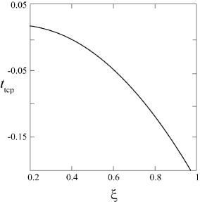
Figure 12: Tricritical temperature $t_{\rm tcp}$ as function of $\xi$, calculated from Eq. (16), for a fixed value of the coupling parameter, $\beta=1$. The analytical expansion is valid only for $\xi$ values that are not too small. In particular, below $\xi=0.2$ the overall change of the phase diagram is from type I to II, as shown in Fig. 11.

At the tricritical point, the free energies for $c=0$ and $c\ll 1$ are equal for the same values of $\phi_{+}$ and $t$. Comparing Eqs. (13) and (9), we obtain the condition for the tricritical point:

$$\delta-t\xi^{-2}-3\xi^{-2}\phi_{+}^{2}=0.$$ (14)

In addition, the spinodal line is obtained from the requirement that $\varepsilon^{\prime\prime}(\phi_{+})=0$ in Eq. (13):

$$3\phi_{+}^{2}\Big{(}1-\frac{9}{\eta}\xi^{-2}\Big{)}+\frac{3}{\eta}\big{(}\delta-t\xi^{-2}\big{)}+2\beta^{2}\xi^{2}+t=0.$$ (15)

By combining Eq. (14) with Eq. (15), we obtain:

$$t_{\rm{tcp}}=\xi^{4}(6\delta\xi^{-2}-\delta\eta-2\beta^{2}\eta)/6,$$ (16)

which depends on the values of $\xi$ and $\beta$. In Fig. 12 we plot the variation of $t_{\rm tcp}$ with respect to $\xi$ for $\beta=1$ and $U/(2\kappa)=1$. Substituting $\beta=1$ and $\xi=0.25$ in Eq. (16), we obtain $\phi_{+}^{\rm tcp}\simeq\pm 0.095$ and $t_{\rm tcp}\simeq 0.014$. These tricritical values are in good agreement with the numerical ones, as can be read off from the phase diagram of Fig. 5(a), $\phi_{+}^{\rm tcp}\simeq\pm 0.094$ and $t_{\rm tcp}\simeq 0.011$.

The present argument is valid only when $c\ll 1$ and can be applied to type I phase diagram for which the domain size should be small (large $\xi$). For type II phase diagram, on the other hand, the tricritical points are located close to the fully-budded phase with $c=2$ (see Fig. 9). In such a case, the expansion in terms of $c$ cannot be justified, and $t_{\rm tcp}(\xi)$ is no more valid for $\xi<0.2$ when $\beta=1$.

References

- (1) B. Alberts, A. Johnson, P. Walter, J. Lewis, and M. Raff, Molecular Biology of the Cell (Garland Science, New York, 2008).
- (2) S. L. Veatch and S. L. Keller, Biochim. Biophys. Acta 1746, 172 (2005).
- (3) S. Komura and D. Andelman, Adv. Coll. Int. Sci. 208, 34 (2014).
- (4) S. L. Veatch and S. L. Keller, Phys. Rev. Lett. 94, 148101 (2005).
- (5) M. Yanagisawa, M. Imai, T. Masui, S. Komura, and T. Ohta, Biophys. J. 92, 115 (2007).
- (6) T. S. Ursell, Bilayer Elasticity in Protein and Lipid Organization (VDM Verlag, Berlin, 2009).
- (7) R. Lipowsky, J. Phys. II (France) 2, 1825 (1992).
- (8) R. Lipowsky, Biophys. J. 64, 1133 (1993).
- (9) J. Hu, T. Weikl, and R. Lipowsky, Soft Matter 7, 6092 (2011).
- (10) F. Jülicher and R. Lipowsky, Phys. Rev. Lett. 70, 2964 (1993).
- (11) F. Jülicher and R. Lipowsky, Phys. Rev. E 53, 2670 (1996).
- (12) R. Lipowsky, Biol. Chem. 395, 253 (2014).
- (13) T. S. Ursell, W. S. Klug, and R. Phillips, Proc. Natl. Acad. Sci. U.S.A. 106, 13301 (2009).
- (14) T. Baumgart, S. T. Hess, and W. W. Webb, Nature 425, 821 (2003).
- (15) J. E. Rim, T. S. Ursell, R. Phillips, and W. S. Klug, Phys. Rev. Lett. 106, 057801 (2011).
- (16) W. Helfrich and R. M. Servuss, Nuovo Cimento 3, 137 (1984).
- (17) R. Lipowsky, M. Brickmann, R. Dimova, C. Haluska, J. Kierfeld, and J. Schillcock J. Phys.: Condens. Matter 17, S2885 (2005).
- (18) S. A. Safran, P. Pincus, and D. Andelman, Science 248, 354 (1990).
- (19) S. A. Safran, P. A. Pincus, D. Andelman, and F. C. MacKintosh, Phys. Rev. A 43, 1071 (1991).
- (20) F. C. MacKintosh and S. A. Safran, Phys. Rev. E 47, 1180 (1993).
- (21) J. L. Harden and F. C. MacKintosh, Europhys. Lett. 28, 495 (1994).
- (22) J. L. Harden, F. C. MacKintosh, and P. D. Olmsted, Phys. Rev. E 72, 011903 (2005).
- (23) W. T. Góźdź and G. Gompper, Europhys. Lett. 55, 587 (2001).
- (24) Y.-S. Ryu, I.-H. Lee, J.-H. Suh, S. C. Park, S. Oh, L. R. Jordan, N. J. Wittenberg, S.-H. Oh, N. L. Jeon, B. Lee, A. N. Parikh, and S.-D. Lee, Nature Comm. 5, 4507 (2014).
- (25) W. Helfrich, Z. Naturforsch. C 28, 693 (1973).
- (26) S. A. Safran, Statistical Thermodynamics of Surfaces, Interfaces, and Membranes, (Addision Wesley, Reading, 1994).
- (27) K. Simons and E. Ikonen, Nature 387, 569 (1997).
- (28) A. Tian, C. Johnson, W. Wang, and T. Baumgart, Phys. Rev. Lett. 98, 208102 (2007).
- (29) M. Blume, V. J. Emery, and R. B. Griffiths, Phys. Rev. A 4, 1071 (1971).
- (30) D. Lingwood and K. Simons, Science 327, 46 (2010).
- (31) M. Seul and D. Andelman, Science 267, 476 (1995).
- (32) S. Leibler and D. Andelman, J. Physique (Paris) 48, 2013 (1987).
- (33) D. Andelman, T. Kawakatsu, and K. Kawasaki Europhys. Lett. 19, 57 (1992).
- (34) T. Taniguchi, K. Kawasaki, D. Andelman, and T. Kawakatsu, J. Phys. II (France) 4, 1333 (1994).
- (35) T. Kawakatsu, D. Andelman, K. Kawasaki, and T. Taniguchi, J. Phys. II (France) 3, 971 (1993).
- (36) H. Kodama and S. Komura, J. Phys. II (France) 3, 1305 (1993).
- (37) P. B. Sunil Kumar, G. Gompper, and R. Lipowsky, Phy. Rev. E 60, 4610 (1999).
- (38) R. Brewster, P. A. Pincus, and S. A. Safran, Biophys. J. 97, 1087 (2009).
- (39) T. Yamamoto, R. Brewster, and S. A. Safran, EPL 91, 28002 (2010).
- (40) B. Palmieri and S. A. Safran, Langmuir 29, 5246 (2013).
- (41) B. Palmieri and S. A. Safran, Langmuir 30, 11734 (2014).
- (42) Y. Hirose, S. Komura, and D. Andelman, Chem. Phys. Chem. 10, 2839 (2009).
- (43) Y. Hirose, S. Komura, and D. Andelman, Phys. Rev. E 86, 021916 (2012).
- (44) R. Shlomovitz, L. Maibaum, and M. Schick, Biophys. J 106, 1979 (2014).
- (45) A. Shioi and T. A. Hatton, Langmuir 18, 7341 (2002).