Generalized extended Lagrangian Born-Oppenheimer molecular dynamics

Abstract

Extended Lagrangian Born-Oppenheimer molecular dynamics based on Kohn-Sham density functional theory is generalized in the limit of vanishing self-consistent field optimization prior to the force evaluations. The equations of motion are derived directly from the extended Lagrangian under the condition of an adiabatic separation between the nuclear and the electronic degrees of freedom. We show how this separation is automatically fulfilled and system independent. The generalized equations of motion require only one diagonalization per time step and are applicable to a broader range of materials with improved accuracy and stability compared to previous formulations.

I Introduction

Born-Oppenheimer molecular dynamics simulations, where classical molecular trajectories are propagated by forces that are calculated on-the-fly from the relaxed electronic ground state in each time step, provide a powerful tool in materials science, chemistry and biology Marx and Hutter (2000); Kirchner et al. (2012). However, the computational cost is high. In regular Born-Oppenheimer molecular dynamics simulations based on Kohn-Sham density functional theory Hohenberg and Kohn (1964); Kohn and Sham (1965); Parr and Yang (1989); Dreizler and Gross (1990), the cost scales with the cube of the number of atoms, which is multiplied by a significant prefactor given by the number of self-consistent field iterations that are required to find the relaxed electronic ground state prior to the force evaluation in each time step. If a sufficient degree of convergence is not achieved, the electronic system behaves like a heat sink or source, gradually draining or adding energy to the atomic system due to a broken time-reversibility in the propagation of the underlying electronic degrees of freedom Remler and Madden (1990); Pulay and Fogarasi (2004); Herbert and Head-Gordon (2005); Niklasson et al. (2006); Kühne et al. (2007). Recently, an extended Lagrangian formulation of Born-Oppenheimer molecular dynamics was proposed that overcomes this problem Niklasson (2008); Steneteg et al. (2010); Zheng et al. (2011); Hutter (2012); Lin et al. (2014); Souvatzis and Niklasson (2014). By including an auxiliary electron density as a dynamical variable, the equations of motion can be integrated without breaking time reversibility, even under approximate self-consistent field convergence. This framework enables Born-Oppenheimer molecular dynamics simulations Cawkwell and Niklasson (2012); Arita et al. (2014) with accurate long-term energy conservation using fast linear scaling solvers Goedecker (1999); Niklasson (2002); Bowler and Miyazaki (2012) that can treat much larger systems than previously possible.

The extended Lagrangian formulation was recently investigated in the limit of vanishing self-consistent field convergence prior to the force calculations. This fast approach requires only one diagonalization per time step Niklasson and Cawkwell (2012); Souvatzis and Niklasson (2013, 2014). In this limit, the iterative ground state optimization, which is necessary in regular Born-Oppenheimer molecular dynamics, is replaced by a dynamical optimization acting over time Bendt and Zunger (1983); Car and Parrinello (1985). However, this fast self-optimizing dynamics relies on the ability to keep the electronic degrees of freedom close to the exact self-consistent ground state, which is approximated using a simple linear mixing. For many materials systems exhibiting, for example, bond breaking or charge sloshing, this linear mixing is insufficient and leads to instabilities. In this article we revisit extended Lagrangian Born-Oppenheimer molecular dynamics in the limit of vanishing self-consistent field optimization and propose a more general formulation that is applicable to a broader range of materials. In contrast to previous formulations we also derive the equations of motion directly from the extended Lagrangian without intermediate steps. This is possible in an adiabatic limit under the condition of a frequency separation between the nuclear and the electronic degrees of freedom, which we show is automatically fulfilled.

We present our generalized extended Lagrangian Born-Oppenheimer molecular dynamics in terms of Kohn-Sham density functional theory Hohenberg and Kohn (1964); Kohn and Sham (1965); Parr and Yang (1989); Dreizler and Gross (1990) and we use the electron density as the variable for the electronic degrees of freedom. However, the framework should be generally applicable also to other electronic structure formulations, for example, density matrices in Hartree-Fock calculations and wavefunctions or Green’s functions in methods for strongly correlated electrons.

II Extended Lagrangian Born-Oppenheimer molecular dynamics

II.1 Generalized extended Born-Oppenheimer Lagrangian

Our generalized extended Born-Oppenheimer Lagrangian is defined by

$$\begin{array}[]{l}{\displaystyle{\cal L}({\bf R},{\bf\dot{R}},n,{\dot{n}})=\frac{1}{2}\sum_{I}M_{I}{\dot{R}}^{2}_{I}-{\cal U}\left({\bf R},n\right)+\frac{1}{2}\mu\int{\dot{n}}^{2}({\bf r})d{\bf r}}\\ {}{}\\ {\displaystyle-\frac{1}{2}\mu{\omega}^{2}\iiint\left(\rho({\bf r}_{1})-n({\bf r}_{1})\right)^{\dagger}K^{\dagger}({\bf r}_{1},{\bf r}_{2})K({\bf r}_{2},{\bf r}_{3})\left(\rho({\bf r}_{3})-n({\bf r}_{3})\right)d{\bf r}_{1}d{\bf r}_{2}d{\bf r}_{3}}.\end{array}$$ (1)

The first term is the kinetic energy for the nuclear degrees of freedom, i.e. the atomic coordinates ${\bf R}=\{R_{I}\}$ and the velocities ${\bf{\dot{R}}}=\{{\dot{R}}_{I}\}$, where the dot denotes the time derivative. The second term is a modified Kohn-Sham Born-Oppenheimer potential energy, ${\cal U}\left({\bf R},n\right)$, including nuclear-nuclear repulsion. A more precise definition of ${\cal U}\left({\bf R},n\right)$ is given in Sec. II.2 below. The last two terms form a harmonic oscillator for the extended electronic degrees of freedom, i.e. the electron density $n({\bf r})$ and its time derivative ${\dot{n}}({\bf r})$. Here $\mu$ is an electron mass parameter and $\omega$ is the frequency determining the curvature of the harmonic well centered around the optimized density $\rho({\bf r})$. The electron density $\rho({\bf r})$ is a fully relaxed and optimized ground state density, but for an approximate linearized electron-electron interaction. Details about the definition of $\rho({\bf r})$ are given below in Sec. II.2. In contrast to the previous formulation of extended Lagrangian Born-Oppenheimer molecular dynamics Niklasson (2008), the harmonic potential includes a non-local kernel $K({\bf r,r^{\prime}})$. This kernel is defined by the relation

$${\displaystyle\int K({\bf r,r^{\prime}})\left(\frac{\delta\rho({\bf r^{\prime}})}{\delta n({\bf r^{\prime\prime}})}-\delta({\bf r^{\prime}-r^{\prime\prime}})\right)d{\bf r^{\prime}}=\delta({\bf r-r^{\prime\prime}})}.$$ (2)

A more detailed explanation for this particular choice, which forces the dynamical variable $n({\bf r})$ to evolve close to the exact fully optimized ground state density, is given in Sec. II.3 below. However, a constant density-independent kernel can also be used.

II.2 Modified Born-Oppenheimer potential energy surface

To construct the modified potential energy surface ${\cal U}\left({\bf R},n\right)$ in Eq. (1), we start with the Kohn-Sham Born-Oppenheimer potential energy surface $U({\bf R})$ Kohn and Sham (1965); Parr and Yang (1989); Dreizler and Gross (1990), which is given by a constrained functional minimization,

$${\displaystyle U({\bf R})=\min_{\widetilde{\rho}}\left\{E({\bf R},{\widetilde{\rho}})~{}\left\lvert~{}{\widetilde{\rho}}({\bf r})=\sum_{i\in{\rm occ}}\left|\psi_{i}({\bf r})\right|^{2},~{}\langle\psi_{i}|\psi_{j}\rangle=\delta_{ij}\right\}\right.+V_{\rm nn}({\bf R})},$$ (3)

where

$${\displaystyle E({\bf R},{\widetilde{\rho}})=\sum_{i\in{\rm occ}}-\frac{1}{2}\langle\psi_{i}|\nabla^{2}|\psi_{i}\rangle+\int V_{\rm ext}({\bf R},{\bf r}){\widetilde{\rho}}({\bf r})d{\bf r}+E_{\rm ee}[{\widetilde{\rho}}].}$$ (4)

The first term in Eq. (4) is the kinetic Kohn-Sham energy for an electron density ${\widetilde{\rho}}({\bf r})$ that is given from an occupied (occ) set of orthonormalized orbitals $\{\psi_{i}\}$. The second term contains the external or pseudopotential potential, $V_{\rm ext}({\bf R},{\bf r})$, i.e. the electron-ion interaction, and the third term is the electron-electron interaction energy,

$$\begin{array}[]{l}{\displaystyle E_{\rm ee}[{\widetilde{\rho}}]=\frac{1}{2}\iint\frac{{\widetilde{\rho}}({\bf r}){\widetilde{\rho}}({\bf r^{\prime}})}{|{\bf r}-{\bf r^{\prime}}|}d{\bf r}d{\bf r^{\prime}}+E_{\rm xc}[{\widetilde{\rho}}]},\\ \end{array}$$ (5)

consisting of the Hartree term and the exchange-correlation energy. The $V_{\rm nn}({\bf R})$ term in Eq. (3) is the ion-ion repulsion energy. The constrained minimization in Eq. (3) is performed over all normalized electron densities, representable by orthonormal orbitals. The minimization defines a ${\widetilde{\rho}}$-independent potential energy surface $U({\bf R})$, which can be calculated through a non-linear iterative self-consistent field optimization procedure that involves solving a sequence of Kohn-Sham eigenvalue equations. The exact self-consistent (sc) ground state density, $\rho_{\rm sc}({\bf r})$, is the density for which the minimum $U({\bf R})$ is obtained in Eq. (3).

The modified Born-Oppenheimer potential energy surface, ${\cal U}({\bf R},n)$ in Eq. (1), is constructed as $U({\bf R})$ if we approximate the electron-electron interaction term $E_{\rm ee}[{\widetilde{\rho}}]$ with a functional linearization around the electron density $n({\bf r})$,

$$\begin{array}[]{l}{\displaystyle E^{(1)}_{\rm ee}[{\widetilde{\rho}},n]=E_{\rm ee}[n]+\left.\int\frac{\delta E_{\rm ee}[{\widetilde{\rho}}]}{\delta{\widetilde{\rho}}}\right\rvert_{{\widetilde{\rho}}=n}\left({\widetilde{\rho}}({\bf r})-n({\bf r})\right)d{\bf r}}.\end{array}$$ (6)

Our modified Born-Oppenheimer potential energy surface is then given by the constrained minimization,

$${\displaystyle{\cal U}({\bf R},n)=\min_{\widetilde{\rho}}\left\{E^{(1)}({\bf R},{\widetilde{\rho}},n)~{}\left\lvert~{}{\widetilde{\rho}}({\bf r})=\sum_{i\in{\rm occ}}\left|\psi_{i}({\bf r})\right|^{2},~{}\langle\psi_{i}|\psi_{j}\rangle=\delta_{ij}\right\}\right.+V_{\rm nn}({\bf R})},$$ (7)

where the electron-electron interaction in Eq. (5) has been replaced by the linearized expression in Eq. (6), i.e.

$${\displaystyle E^{(1)}({\bf R},{\widetilde{\rho}},n)=\sum_{i\in{\rm occ}}-\frac{1}{2}\langle\psi_{i}|\nabla^{2}|\psi_{i}\rangle+\int V_{\rm ext}({\bf R},{\bf r}){\widetilde{\rho}}({\bf r})d{\bf r}+E^{(1)}_{\rm ee}[{\widetilde{\rho}},n].}$$ (8)

The density $n({\bf r})$ appears in ${\cal U}({\bf R},n)$ as a dynamical variable in the same way as ${\bf R}$. A given set of dynamical variables, $n({\bf r})$ and ${\bf R}$, determine the relaxed optimized ground state density $\rho({\bf r})$, which is attained at the minimum that defines ${\cal U}({\bf R},n)$ in Eq. (7), in the same way as the non-linear iterative optimization of regular Kohn-Sham density functional theory determines the exact self-consistent ground state density $\rho_{\rm sc}({\bf r})$ in Eq. (3), i.e.

$${\displaystyle\rho({\bf r})=\arg\min_{\widetilde{\rho}}\left\{E^{(1)}({\bf R},{\widetilde{\rho}},n)~{}\left\lvert~{}{\widetilde{\rho}}({\bf r})=\sum_{i\in{\rm occ}}\left|\psi_{i}({\bf r})\right|^{2},~{}\langle\psi_{i}|\psi_{j}\rangle=\delta_{ij}\right\}\right.}.$$ (9)

The main difference is that the constrained minimum of the linearized form in Eq. (7) or (9) can be obtained from a single solution of a regular Kohn-Sham eigenvalue equation with the Kohn-Sham Hamiltonian $H_{\rm KS}[n]$ calculated at density $n({\bf r})$, i.e.

$$\rho[n]({\bf r})=\sum_{i\in\rm occ}|\psi_{i}({\bf r})|^{2},~{}~{}~{}{\rm where}~{}~{}~{}H_{\rm KS}[n]\psi_{i}({\bf r})=\varepsilon_{i}\psi_{i}({\bf r}).{\displaystyle}$$ (10)

To highlight this direct relationship between the optimized electron density $\rho({\bf r})$ from Eq. (9) and the dynamical variable density $n({\bf r})$ we may use the equivalent notation $\rho[n]({\bf r})\equiv\rho({\bf r})$, as above. The leading difference between the modified potential energy surface ${\cal U}({\bf R},n)$ and the regular Kohn-Sham potential $U({\bf R})$, which follows from the linearization, is of second order with respect to the error in the density. As long as the dynamical variable density $n({\bf r})$ evolves close to the exact ground state density $\rho_{\rm sc}({\bf r})$, the difference between the modified potential energy surface ${\cal U}({\bf R},n)$ and the exact Kohn-Sham potential $U({\bf R})$ will be small. This motivates our specific choice of the generalized kernel in Eq. (2) as will be shown in the next section.

II.3 Ground state optimization kernel

Our particular choice of the generalized kernel $K({\bf r},{\bf r^{\prime}})$ in Eq. (2) forces the dynamical variable density $n({\bf r})$ to evolve close to the exact self-consistent ground state density $\rho_{\rm sc}({\bf r})$, such that the modified Born-Oppenheimer potential energy surface ${\cal U}({\bf R},n)$ is an accurate approximation to the regular self-consistent Kohn-Sham potential $U({\bf R})$.

Let the functional $F(n)$ be the difference between $\rho[n]({\bf r})$ and $n({\bf r})$, i.e.

$${\displaystyle F(n)=\rho[n]-n.}$$ (11)

The equation $F(n)=0$ is fulfilled for the exact self-consistent ground state density, i.e. when $n({\bf r})=\rho_{\rm sc}({\bf r})$. If $n({\bf r})$ is sufficiently close to the exact ground state density $\rho_{\rm sc}({\bf r})$, we may approximate the ground state density through a Newton minimization step Nocedal and Wright (1990), which schematically is given by

$${\displaystyle\rho_{\rm sc}\approx n-{\cal J}^{-1}F(n),}$$ (12)

where ${\cal J}$ is the Jacobian, $\delta F/\delta n$. This means that

$${\displaystyle\rho_{\rm sc}-n\approx-{\cal J}^{-1}\left(\rho[n]-n\right)}$$ (13)

or in a more explicit form

$${\displaystyle\rho_{\rm sc}({\bf r})-n({\bf r})\approx-\int K({\bf r},{\bf r^{\prime}})\left(\rho[n]({\bf r^{\prime}})-n({\bf r^{\prime}})\right)d{\bf r^{\prime}},}$$ (14)

where the non-local operator $K({\bf r},{\bf r^{\prime}})$ is the inverse Jacobian of $F(n)=\rho[n]-n$ defined by

$${\displaystyle\int K({\bf r,r^{\prime}})\left(\frac{\delta\rho({\bf r^{\prime}})}{\delta n({\bf r^{\prime\prime}})}-\frac{\delta n({\bf r^{\prime}})}{\delta n({\bf r^{\prime\prime}})}\right)d{\bf r^{\prime}}=\delta({\bf r-r^{\prime\prime}})},$$ (15)

which corresponds to our definition of the kernel in Eq. (2). The error in the approximation in Eq. (14), at least under reasonable conditions, is of second order, i.e. ${\cal O}\left((\rho-n)^{2}\right)$, which can be understood from the quadratic convergence of the Newton scheme for sufficiently close initial values of $n$ and assuming $F(n)$ is smooth Nocedal and Wright (1990). Our particular choice of the non-local kernel in the generalized extended Lagrangian, Eq. (1), is thus derived from an optimization of the extended harmonic potential to accurately mimic the oscillation of $n({\bf r})$ around the exact ground state density $\rho_{\rm sc}({\bf r})$. This improves the accuracy of the modified potential energy surface ${\cal U}({\bf R},n)$ and helps stabilize the dynamics.

II.4 Equations of motion

Previous derivations of the equations of motion in the limit of vanishing self-consistent field convergence Souvatzis and Niklasson (2013, 2014) started from the decoupled equations of motion of extended Lagrangian Born-Oppenheimer molecular dynamics in the limit of full self-consistent field convergence. Then, a simplified set of equations of motion were derived by relaxing the condition of the self-consistent field optimization. Such an approach can be difficult to interpret. Here we will follow a more direct path in the derivation, without assuming an intermediate step of full self-consistent field convergence. Instead, we will apply an adiabatic condition that assumes a separation in the frequencies between the nuclear and the electronic degree of freedom.

The Euler-Lagrange equations of motion for the generalized extended Lagrangian, ${\cal L}({\bf R},{\bf\dot{R}},n,{\dot{n}})$ in Eq. (1), describe a coupled dynamical system of nuclear degrees of freedom with some unknown highest characteristic frequency $\Omega$ and an electronic degrees of freedom with the frequency $\omega$. For normal integration time steps used in regular Born-Oppenheimer molecular dynamics we will show in Sec. II.7 that $\omega>\Omega$ and that we have a natural system-independent adiabatic separation between the two frequencies. This natural adiabatic separation between slower nuclear and faster electronic degrees of freedom motivates our derivation of the equation of motion in the limit when $\omega^{2}/\Omega^{2}\rightarrow\infty$. In this limit the difference between $\rho({\bf r})$ and $n({\bf r})$ is small and scales as the inverse of the square of the electron frequency $\omega^{2}$, i.e. $(\rho[n]-n)={\cal O}(\Omega^{2}/\omega^{2})$. This assumed scaling of $(\rho[n]-n)$ as a function of $\omega^{2}/\Omega^{2}\rightarrow\infty$ is difficult to prove rigorously, but it is straightforward to demonstrate that it holds a posteriori (See Fig. 3). In this adiabatic limit we further choose to reduce the electron mass parameter $\mu\rightarrow 0$ such that $\lim\mu\omega\rightarrow{\rm constant}$. The Euler-Lagrange equations of motion in this limit are

$$\begin{array}[]{l}{\displaystyle M_{I}{\ddot{R}}_{I}=-\left.\frac{\partial{\cal U}\left({\bf R},n\right)}{\partial R_{I}}\right\lvert_{n},}\\ {}{}\\ {\displaystyle{\ddot{n}}({\bf r})=-\omega^{2}\int K({\bf r},{\bf r^{\prime}})\left(\rho({\bf r^{\prime}})-n({\bf r^{\prime}})\right)d{\bf r^{\prime}}},\end{array}$$ (16)

where the forces in the first equation are given from the partial derivative of ${\cal U}({\bf R},n)$ under the condition of a constant density $n({\bf r})$, since it is a dynamical variable, and where $K({\bf r},{\bf r^{\prime}})$ is defined by Eq. (2). A more detailed derivation of the equations of motion is given in the appendix.

The modified Born-Oppenheimer potential energy surface ${\cal U}({\bf R},n)$ is calculated through a single diagonalization, which yields the optimized density $\rho({\bf r})$, Eq. (10). No additional diagonalization of the Kohn-Sham Hamiltonian is necessary to integrate the equations of motion above – only one Hamiltonian diagonalization per molecular dynamics time step is necessary. However, the additional calculation of the kernel $K({\bf r},{\bf r^{\prime}})$ may introduce a significant overhead.

The key results of this paper are the equations of motion, Eq. (16), and their derivation from the generalized extended Lagrangian, Eq. (1), under the condition of an adiabatic separation between the frequencies of the nuclear and the electronic degrees of freedom. This allows stable molecular dynamics simulations for a broader range of materials systems than previously possible. The extended range of systems that can be treated with the new generalized formalism can be understood from the stability conditions of our previous formulation of extended Lagrangian Born-Oppenheimer molecular dynamics, as will be discussed in the next section.

II.5 Stability

It is easy to see that previous formulations of extended Lagrangian Born-Oppenheimer molecular dynamics in the limit of vanishing self-consistent field optimization Niklasson and Cawkwell (2012); Souvatzis and Niklasson (2013, 2014) are recovered with a scaled $\delta$-function approximation of the kernel, i.e. for $K({\bf r},{\bf r^{\prime}})=-c~{}\delta({\bf r-r^{\prime}})$ in Eq. (16), where $c\in[0,1]$. This corresponds to approximating the exact ground state density $\rho_{\rm sc}({\bf r})$ by a simple linear mixing, i.e. where

$${\displaystyle\rho_{\rm sc}({\bf r})\approx c\rho({\bf r})+(1-c)n({\bf r}),}$$ (17)

so that

$${\displaystyle\rho_{\rm sc}({\bf r})-n({\bf r})\approx c\left(\rho({\bf r})-n({\bf r})\right).}$$ (18)

The equation of motion for the electronic degrees of freedom with the scaled $\delta$-function approximation of the kernel in Eq. (16),

$${\displaystyle{\ddot{n}}({\bf r})=c\omega^{2}\left(\rho({\bf r})-n({\bf r})\right),}$$ (19)

therefore corresponds to a dynamics where the auxiliary density $n({\bf r})$ evolves around a self-consistent ground state density that is approximated by a linear mixing between $\rho[n]$ and $n$. This linear mixing provides a reasonable approximation of the self-consistent ground state density if the electronic energy functional $E({\bf R},{\widetilde{\rho}})$ has a simple convex form, such that

$${\displaystyle E\left({\bf R},c\rho+(1-c)n\right)<cE\left({\bf R},\rho\right)+(1-c)E\left({\bf R},n\right),~{}~{}~{}c\in[0,1].}$$ (20)

This allows a stable integration of the electronic degrees of freedom in Eq. (16) using the local scaled $\delta$-function approximation of the kernel and requires only one Kohn-Sham diagonalization per time step. However, instabilities may occur, for example, during bond breaking or in large metallic systems exhibiting charge sloshing. In this case $\rho({\bf r})$ has to be further updated through an iterative self-consistent field optimization. Thus, while previous formulations, in the limit requiring only one diagonalization per time step, rely on stability and convergence using a constant linear mixing, which is possibly guaranteed only for convex functionals Dederichs and Zeller (1983), the generalized formulation with a non-local kernel will have a broader range of applications. We can expect that the difference in applicability should be related to the range of systems for which a simple constant linear mixing between densities is sufficient to reach the self-consistent ground state solution in a regular Kohn-Sham calculation Dederichs and Zeller (1983), in comparison to problems where Newton-like iterations, such a Broyden or Kerker mixing are necessary Broyden (1965); Srivastava (1984); Johnson (1988); Kerker (1981).

II.6 Constant of motion

The constrained optimization of ${\widetilde{\rho}}({\bf r})$ in Eq. (9) that defines ${\cal U}({\bf R},n)$ in Eq. (7) and thus the nuclear forces in Eq. (16), corresponds to a ground state relaxation of the electronic degrees of freedom with respect to the regular Kohn-Sham energy functional as in Eq. (3), but with a linearized expression for the electron-electron interaction, Eq. (6). In this way ${\cal U}({\bf R},n)$ as defined by Eq. (7) can be understood in terms of an optimized and thus ${\widetilde{\rho}}$-independent Born-Oppenheimer potential energy surface with a relaxed electron density, but which, thanks to the linearized electron-electron interaction term, can be obtained through a single diagonalization, Eq. (10). We may therefore interpret our one-diagonalization-per-time-step extended Lagrangian Born-Oppenheimer molecular dynamics as an exact Kohn-Sham Born-Oppenheimer molecular dynamics simulation, but with a constant of motion of a modified shadow Hamiltonian,

$${\displaystyle E_{\rm Tot}=\frac{1}{2}\sum_{I}M_{I}{\dot{R}}_{I}+{\cal U}({\bf R},n)},$$ (21)

which is valid in the same adiabatic limit as the equations on motion, Eq. (16). Thus, instead of integrating the exact Kohn-Sham Born-Oppenheimer equations of motion using an approximate self-consistent field optimization that leads to a systematic drift in the energy Remler and Madden (1990); Pulay and Fogarasi (2004), we perform the integration based on an exact, fully optimized ground state density but for an approximate shadow Hamiltonian. In this way the energy drift of regular Born-Oppenheimer molecular dynamics can be avoided. The argument is conceptually very similar to the backward analysis for symplectic integration schemes Engel et al. (2005). As long as $\rho({\bf r})$ and $n({\bf r})$ are close to the self-consistent ground state density $\rho_{\rm sc}({\bf r})$, $E_{\rm Tot}$ and the potential energy surface ${\cal U}({\bf R},n)$ will be very close to exact Kohn-Sham Born-Oppenheimer molecular dynamics. This condition is automatically fulfilled when there is an adiabatic separation between $\rho({\bf r})$ and $n({\bf r})$. As will be shown in the next section, this separation is naturally fulfilled and material independent.

II.7 Adiabatic separation

Under the condition of an adiabatic separation between a slower nuclear motion characterized by a frequency $\Omega$, and a faster auxiliary electronic motion governed by the frequency of the extended harmonic oscillator $\omega$, we may expect, based on the classical adiabatic theorem, that the dynamical variable density $n({\bf r})$, which is controlled by the harmonic oscillator frequency $\omega$, closely should follow the exact ground state density $\rho_{\rm sc}({\bf r})$, which is governed by a slower nuclear frequency $\Omega$. As we will show here, this condition of adiabatic separation between $\Omega$ and $\omega$ is automatically fulfilled. We can make a straightforward estimate of this separation assuming a standard Verlet integration of $n({\bf r})$ in the equations of motion in Eq. (16),

$${\displaystyle n({\bf r},t+\delta t)=2n({\bf r},t)-n({\bf r},t-\delta t)-\delta t^{2}\omega^{2}\int K({\bf r},{\bf r^{\prime}})\left(\rho({\bf r^{\prime}})-n({\bf r^{\prime}})\right)d{\bf r^{\prime}}.}$$ (22)

It can be shown that the highest possible value of the dimensionless variable $\kappa=\delta t^{2}\omega^{2}$ that provides a stable Verlet integration is for $\kappa=2$ Niklasson (2008); Niklasson et al. (2009); Steneteg et al. (2010). For higher order symplectic integration schemes, significantly larger values of $\kappa$ are possible Odell et al. (2009), though these schemes require multiple force evaluations per time step. We further assume that the shortest period of the nuclear degrees of freedom, $T_{n}$ (with the corresponding frequency $\Omega$), is integrated in about 20 integration time steps such that $\delta t=T_{n}/20$, which is a reasonable choice both in classical and regular Born-Oppenheimer molecular dynamics simulations. In this case we have that

$$\frac{\Omega}{\omega}=\frac{2\pi/T_{n}}{\omega}=\frac{2\pi/(20\delta t)}{\sqrt{2}/\delta t}=\frac{2\pi}{20\sqrt{2}},$$ (23)

i.e. $\omega\approx 4.5\times\Omega$. Thus, for a normal choice of integration time step as used in classical or regular Born-Oppenheimer molecular dynamics, we have a natural and system independent separation between the faster extended harmonic oscillator frequency $\omega$ and the slower nuclear frequency $\Omega$. It is this natural adiabatic separation that motivates the derivation of the equations of motion in the adiabatic limit when $\omega^{2}/\Omega^{2}\rightarrow\infty$. The ratio that governs the error, i.e. $\Omega^{2}/\omega^{2}\approx 1/20$, may seem large to motivate the full adiabatic limit. However, as we will demonstrate in the examples below, this natural and material independent separation is sufficient to provide highly accurate molecular dynamics simulations.

III Examples

We have performed an implementation of our generalized extended Lagrangian Born-Oppenheimer dynamics in the self-consistent charge density functional based tight-binding code LATTE Cawkwell and Niklasson (2012); Niklasson and Cawkwell (2012). It has a particularly simple form that allows a direct calculation of the exact non-local kernel. In density functional based tight-binding theory Elstner et al. (1998); Finnis et al. (1998); Frauenheim et al. (2000); Aradi et al. (2007) the continuous charge density $n({\bf r})$ is represented by the atomic net Mulliken charges ${\bf n}=\{n_{i}\}$ for each atom $i$. In the same way, the optimized ground state density $\rho({\bf r})$ is represented by net Mulliken charges ${\bf q}=\{q_{i}\}$. In this formalism the generalized electronic equations of motion in Eq. (16) are given by

$${\displaystyle{\ddot{n}}_{i}=-\omega^{2}\sum_{j}K_{ij}\left(q_{j}-n_{j}\right)},$$ (24)

where the kernel is calculated from

$${\displaystyle\sum_{j}K_{ij}{\cal J}_{jk}=\delta_{ik}},$$ (25)

with

$${\displaystyle{\cal J}_{jk}=\frac{\delta q_{j}}{\delta n_{k}}-\delta_{jk}.}$$ (26)

The derivatives $\delta q_{j}/\delta n_{k}$ have been calculated using density matrix perturbation theory Niklasson and Challacombe (2004) and the nuclear degrees of freedom have been integrated using the velocity Verlet algorithm. For the electronic degrees of freedom we used a modified Verlet integration scheme Niklasson et al. (2009); Steneteg et al. (2010); Zheng et al. (2011), where

$${\displaystyle n_{i}(t+\delta t)=2n_{i}(t)-n_{i}(t-\delta t)+\delta t^{2}{\ddot{n}}_{i}(t)+\alpha\sum_{k=0}^{K}c_{k}n_{i}(t-k\delta t).}$$ (27)

This integration scheme is neither symplectic nor exactly time-reversible when $\alpha>0$. However, without the last dissipative force term in the integration scheme, accumulation of numerical noise may lead to instabilities.

The equations of motion in previous formulations Niklasson and Cawkwell (2012); Souvatzis and Niklasson (2013, 2014) are recovered by a scaled $\delta$-function approximation of the $\delta q/\delta n$ derivative, where $\delta q_{j}/\delta n_{k}\sim\delta_{jk}$. In this case the equations of motion are simplified to

$${\displaystyle{\ddot{n}}_{i}=c\omega^{2}\left(q_{i}-n_{i}\right)},~{}~{}~{}c\in[0,1].$$ (28)

As was previously discussed in Sec. II.5, this corresponds to a harmonic oscillator evolving around a ground state density that is approximated by a linear mixing. As long as linear mixing gives an improved ground state estimate over $n({\bf r})$, this is a simple, efficient and stable approach. For many systems there is therefore no visible effect if we switch from the scaled $\delta$-function approximation to the exact calculation of the non-local kernel in Eq. (2). However, for material systems where a simple constant linear mixing is not sufficient to reach a ground state solution the previous approach will fail. For such systems (or if the scaling constant $c$ has been set too large or too small) instabilities occur in the time integration of $n({\bf r})$ and the simulations may diverge. In this case multiple self-consistent field iterations using some more advanced optimization scheme are necessary to improve the approximation of $\rho({\bf r)}$, which significantly increases the computational cost.

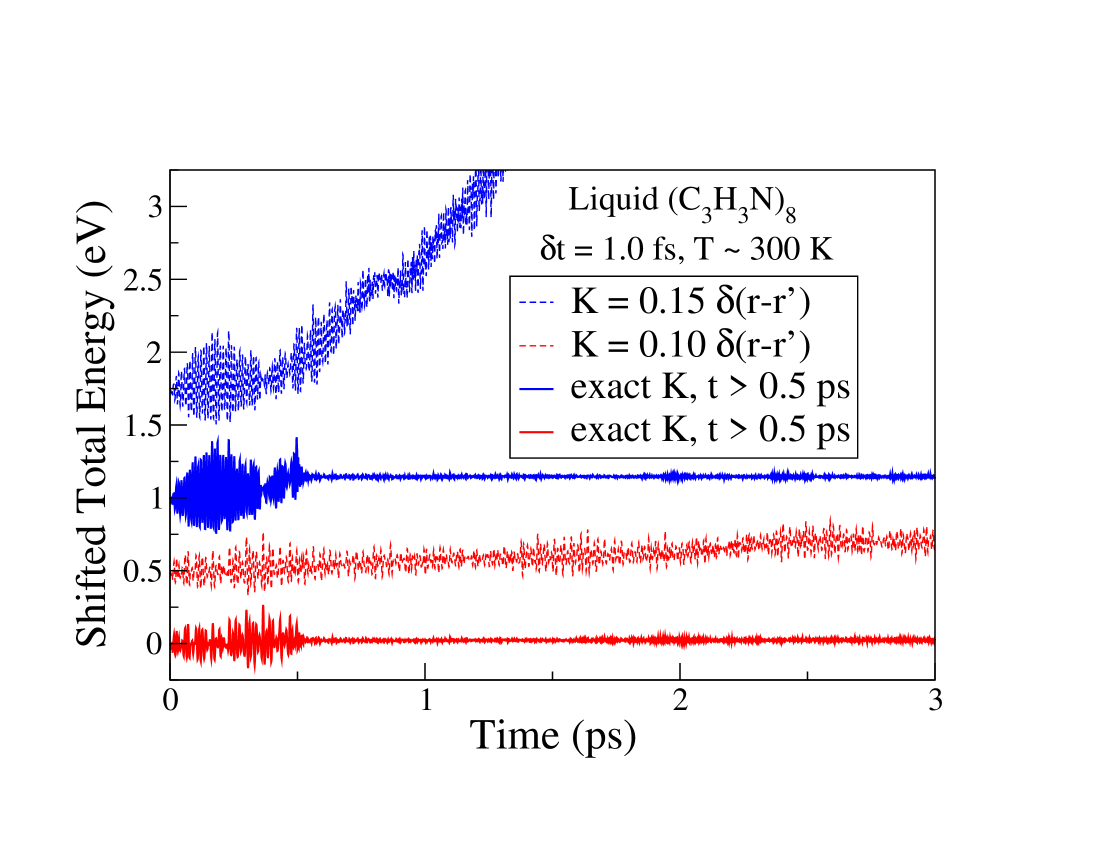
Figure 1: (color online) The fluctuations of the shifted total (kinetic+potential) Born-Oppenheimer energy, $E_{\rm Tot}$ in Eq. (21), for simulations of liquid acrylinitrile (C₃H₃N) using only one diagonalization per time step with various approximations of the kernel, $K({\bf r},{\bf r^{\prime}})$ in Eq. (2), for the generalized extended Lagrangian Born-Oppenheimer molecular dynamics, Eq. (16). The two dashed curves illustrate two scaled $\delta$-function approximations of the kernel. The two solid lines show the same simulations until $t=0.5$ ps when we switch from the scaled $\delta$-function approximations to the exact non-local kernel. The exact non-local kernel, Eq. (2), which is calculated at $t=0.5$ ps and then kept constant for $t>0.5$ ps, provides a very accurate dynamics, which is very close to an exact regular Born-Oppenheimer molecular dynamics.

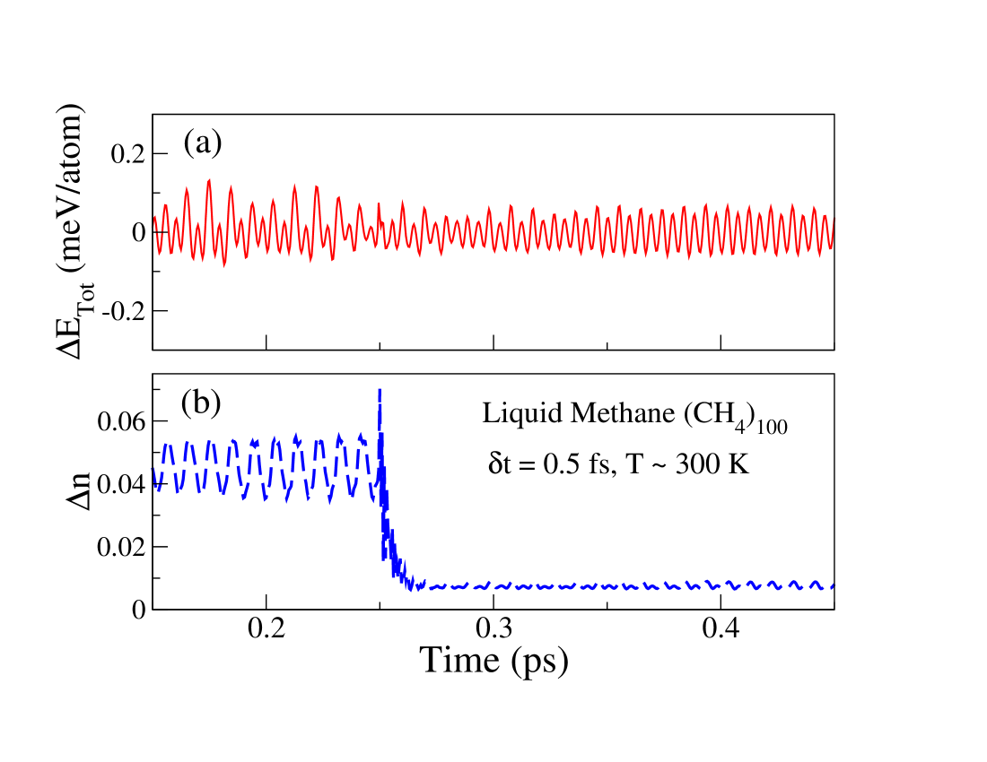
Figure 2: (color online) The upper panel (a) shows fluctuations of the shifted total (kinetic+potential) Born-Oppenheimer energy, Eq. (21), for a simulation of liquid methane at room temperature. The lower panel (b) shows the fluctuations of the 2-norm error in the charge, $\Delta n=\|n({\bf r})-\rho_{\rm sc}({\bf r})\|_{2}$, between the auxiliary dynamical variable density and the exactly optimized self-consistent ground state. The kernel, $K({\bf r},{\bf r^{\prime}})$, is approximated with a scaled $\delta$-function, $K({\bf r},{\bf r^{\prime}})=-0.25~{}\delta({\bf r-r^{\prime}})$, for $t<0.25$ ps and with the constant non-local kernel, Eq. (2), for $t\geq 0.25$ ps. All calculations of the charges where performed in a single step directly from the effective Kohn-Sham Hamiltonian, Eq. (10), using a linear scaling density matrix expansion scheme Niklasson (2002); Cawkwell and Niklasson (2012).

Figure 1 depicts some results of using various approximations to the kernel $K({\bf r},{\bf r^{\prime}})$ in Eq. (2) for simulations of liquid acrylonitrile. Only one Hamiltonian diagonalization (or density matrix construction) per time step was used. Liquid acrylonitrile (C₃H₃N) was chosen because it shows significant instabilities with a dynamics that is hard to stabilize with a simple scaled $\delta$-function approximation of the kernel $K({\bf r,r^{\prime}})$. The two solid curves show what happens when we switch from a simple scaled $\delta$-function approximation to the exact non-local expression in Eq. (2), which thereafter is kept constant after its calculation at $t=0.5$ ps. The two dashed lines show the fluctuations in the total energy if we continue using the scaled $\delta$-function approximation. As is clearly seen, the exact non-local kernel provides a very efficient stabilization of the dynamics even if it is kept fixed as a constant preconditioner after its initial calculation. In fact, recalculating the kernel for each new time step (not shown) makes very little difference to the simulation in Fig. 1. This indicates that it is possible to use more efficient, approximate calculations of the kernel in the first place, possibly Broyden based schemes Broyden (1965); Srivastava (1984); Johnson (1988), of Kerker mixing techniques Kerker (1981), as well as other more recent methods Anglade and Gonze (2008); Lin and Yang (2013) with similar results. These optimization schemes that are used in a broad range of self-consistent electronic structure methods are based on various non-local approximations of the exact kernel and reduces the computational cost significantly Nocedal and Wright (1990).

The upper panel of Fig. 2 shows the fluctuations in the total energy for a simulation of liquid methane. The effect on the total energy fluctuations from the exact non-local kernel, which is included at $t=0.25$ ps, is fairly small. However, the error in the charge distribution (lower panel) shows a significant shift, but the error is small already at $t<0.25$ ps when the local scaled $\delta$-function approximation is used for the kernel. The $\delta$-function approximation was scaled with an artificially small prefactor, $c=0.25$, to enhance the effect of the switch to the non-local exact kernel. If a prefactor in the range of $c\in[0.5,0.7]$ had been chosen, the difference would have been much smaller.

The computational cost of calculating the exact kernel in Eq. (2) increases with the number of atoms such that a system with 100 atoms introduces an additional effort in a single calculation of $K({\bf r,r^{\prime}})$ corresponding to about 100 normal molecular dynamics time steps without the calculation of $K({\bf r,r^{\prime}})$. Fortunately, the calculation is trivially parallelizable and may thus add very little overhead in the total wall-clock time of a simulation, in particular, if the kernel only needs to be updated every few thousand time steps. However, for simulations of very large systems, which may require a more frequent update of the kernel, the full exact calculation of $K({\bf r,r^{\prime}})$ has to be avoided.

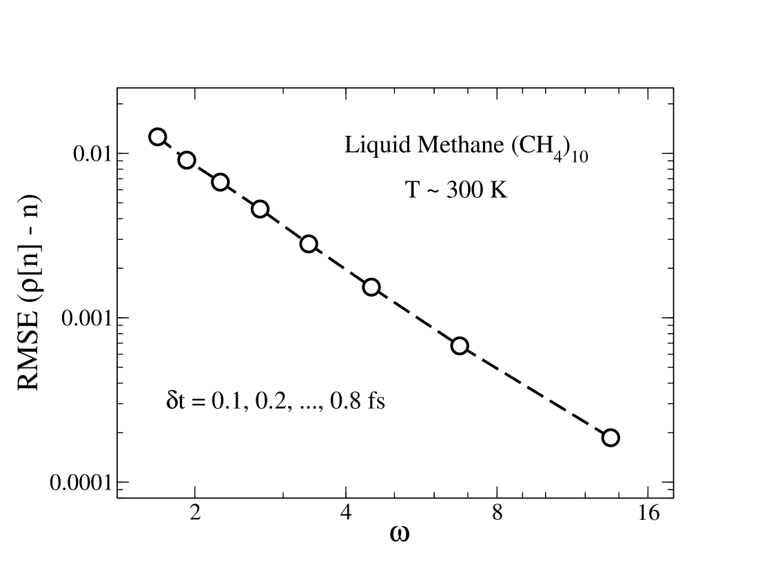
Figure 3: (color online) The root mean square error (RMSE) or the difference between $\rho[n]({\bf r})$ and $n({\bf r})$ in a simulation of liquid methane as a functions of $\omega$. The RMSE scales as $\omega^{-2}$. The simulations were performed for a sequence of integration time step $\delta t=0.1,0.2,\ldots,0.8$ fs.

In Fig. 3 we demonstrate the scaling of the difference between $\rho[n]({\bf r})$ and $n({\bf r})$ as a function of $\omega$. The exact non-local kernel was calculated once in the beginning of the simulations and was thereafter kept constant. The root mean square error between $\rho[n]({\bf r})$ and $n({\bf r})$ was calculated for 2,000 time steps. Since $\delta t^{2}\omega^{2}=\kappa$, which occurs as a constant dimensionless factor in the modified Verlet integration, Eq. (22) or (27), we have that $\omega={\sqrt{\kappa}}/\delta t$. Different values of $\omega$ are thus given by modifying the integration time step $\delta t$. The figure clearly demonstrates how the difference between $\rho[n]({\bf r})$ and $n({\bf r})$ scales as $\omega^{-2}$, which is consistent with the necessary assumption in the derivation of the equations of motion in the adiabatic limit as $\omega\rightarrow\infty$. This also illustrates the tunable accuracy of the simulation. Since $\rho[n]({\bf r})-n({\bf r})=F(n)$ in Eq. (11), the dynamics converges quadratically toward exact self-consistent Kohn-Sham Born-Oppenheimer molecular dynamics as $\omega\rightarrow\infty$. However, already for a normal integration time step when $\delta t=0.5$ fs, the root mean square error is less than $0.005$.

The sensitivity to the integration time step and the value of $\omega$ can also be investigated for the vibrational spectra. Figure 4 shows the (shifted) vibrational density of states (DOS) of liquid Methane given from the Fourier transform of the velocity autocorrelation function Dickey and Paskin (1969). After an initial equilibration of 50,000 time steps the velocity autocorrelation was sampled over 100,000 time steps every femtosecond for simulations using four different integration time steps $\delta t$. The lower curves show the results for Born-Oppenheimer molecular dynamics simulations using multiple self-consistent field iterations in the optimization of the ground state density before each force evaluation (“exact” BOMD). The four upper curves show the same results using our fast generalized extended Lagrangian formulation that requires only one diagonalization per MD time step with the optimized non-local kernel. The curves are virtually all on top of each other without any sensitivity to $\omega$ in for range of integration time steps. The longest integration time step, $\delta t=0.6$ ps, is about 1/20 of the shortest period corresponding to the highest frequency of the system. For time steps $\delta t=0.75$ ps we started to se an instability with a small but systematic drift in the energy both for the optimized Born-Oppenheimer simulation and the extended Lagrangian scheme with the non-local kernel.

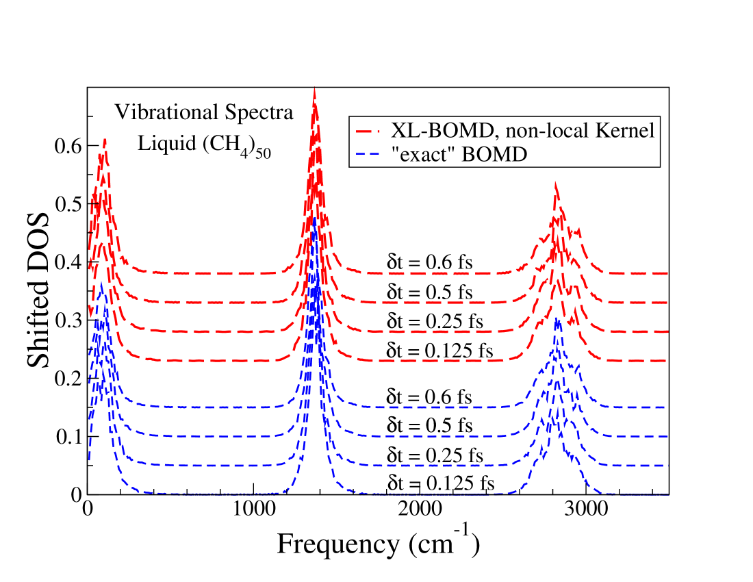
Figure 4: (color online) The vibrational density of states (DOS) for liquid methane calculated from the velocity autocorrelation function that was sampled using either Born-Oppenheimer molecular dynamics with an optimized ground state density prior to each force evaluation (“exact” BOMD) or the fast generalized extended Lagrangian formulation that requires only diagonalization per MD time step (XL-BOMD) with the optimized non-local kernel $K({\bf r,r^{\prime}})$ in Eq. (2). Four different integration time steps $\delta t$ were used with a temperature initialized to 300 K during equilibration.

IV Discussion

The generalized extended Lagrangian formulation of Born-Oppenheimer molecular dynamics allows a more accurate and stable dynamics for a broader class of systems. Calculations involving bond breaking or charge sloshing, which may occur in simulations of chemical reactions or large metallic systems, are often not possible to converge using a simple constant linear mixing of densities. The generalized non-local kernel acting on the electronic degrees of freedom can avoid such shortcomings and thus significantly increase the application range of extended Lagrangian Born-Oppenheimer molecular dynamics simulations in the fast limit that only requires one diagonalization per time step.

The derivation of the generalized equations of motion based on the adiabatic condition has several connections to the analysis of the equations of motion of extended Born-Oppenheimer molecular dynamics in its original formulation that recently was performed by Lin et al. Lin et al. (2014) as well as the more generalized framework described by Hutter Hutter (2012). Their analysis also includes several interesting comparisons and relations to Car-Parrinello molecular dynamics Car and Parrinello (1985); Tuckerman et al. (1996); Marx and Hutter (2000), which is based on an extended Lagrangian approach to first principles molecular dynamics simulations that was introduced almost 30 years ago.

The concept of a modified shadow Hamiltonian plays an important role in classical molecular dynamics Channel and Scovel (1990); McLachlan and Atela (1992); Leimkuhler and Reich (2004); Engel et al. (2005). Instead of an approximate numerical integration of an underlying exact Hamiltonian dynamics, a class of symplectic integration schemes corresponds to an exact numerical integration of an underlying approximate shadow Hamiltonian. In this way properties of the dynamical flow of a Hamiltonian dynamics can be rigorously conserved. Here we used the concept of a shadow Hamiltonian in the context of an incomplete self-consistent field optimization to describe and understand the accuracy in the long-term conservation of the total energy.

Although conceptually different and presented in a form that is easy to generalize to other functionals, the modified Born-Oppenheimer potential energy surface ${\cal U}({\bf R},n)$ with the linearized electron-electron interaction in Eq. (7) has the same form as the Harris-Foulkes functional Harris (1985); Foulkes and Haydock (1989), with a second-order error term

$${\displaystyle{\cal U}({\bf R},n)-U({\bf R})={\cal O}\left((\rho-\rho_{\rm sc})(n-\rho_{\rm sc})\right).}$$ (29)

The main difference is that ${\cal U}({\bf R},n)$ is represented in terms of a variationally optimized energy functional for a given external and electrostatic potential that are determined by the nuclear positions ${\bf R}$ and a dynamical variable density $n({\bf r})$. Since $n({\bf r})$ occurs as a dynamical variable in the extended Lagrangian, forces that are calculated from the Euler-Lagrange equations of motion are given by partial derivatives of ${\cal U}({\bf R},n)$ with respect to a constant density $n({\bf r})$ in Eq. (16). This is not possible in a Harris-Foulkes functional, where $n({\bf r})$ represents either overlapping ${\bf R}$-dependent atomic charge densities or the successive (non-converged and thus ${\bf R}$-dependent) input densities in a regular iterative Kohn-Sham optimization procedure. Thus, our modified Born-Oppenheimer potential energy surface ${\cal U}({\bf R},n)$ plays a quite different role and allows computationally simple and accurate calculations of the forces without relying on the Hellmann-Feynman theorem Marx and Hutter (2000).

The important role of $n({\bf r})$ as a dynamical variable is sometimes misunderstood. It is only thanks to the underlying dynamical framework that our molecular dynamics simulations work. Extended Lagrangian Born-Oppenheimer molecular dynamics is sometimes referred to simply as a time-reversible extrapolation scheme for the electronic degrees of freedom from one step to the next. That picture is misleading in the same way as if we would view extended Lagrangian Car-Parrinello molecular dynamics simply as an ad hoc numerical interpolation technique for wavefunctions.

The calculations of the exact non-local kernel $K({\bf r,r^{\prime}})$ increases the computational cost of extended Lagrangian Born-Oppenheimer molecular dynamics. However, for many systems a local scaled $\delta$-function approximation is sufficient. Other approximate expressions based on, for example, Broydens method or Kerker mixing could also be applied. In fact, it is straightforward to invent numerous flavors of local or semi-local approximations of the Kernel that require different levels of computational complexity. However, each update of an approximate Kernel, for example based on the Broyden scheme, would introduce a computational overhead similar to a full self-consistent field optimization. An understanding of the efficiency of various existing non-local kernel approximations can be estimated from their previous applications to accelerate the self-consistent field optimization in regular Kohn-Sham density functional theory with a fixed external potential Broyden (1965); Dederichs and Zeller (1983); Srivastava (1984); Johnson (1988); Anglade and Gonze (2008); Lin and Yang (2013). However, there is exist no perfect, fully automatic, black box solution to the self-consistent field optimization problem and the same limitation can therefore be expected also for application in the generalized form of extended Lagrangian Born-Oppenheimer molecular dynamics.

V Summary and conclusions

We have proposed a generalized framework for extended Lagrangian Born-Oppenheimer molecular dynamics, Eqs. (1) and (16), that improves the stability and extends the range of applications in the limit of fast quantum based molecular dynamics simulations that require only one diagonalization per time step. We showed how the equations of motion, Eq. (16), can be derived directly from the Lagrangian, Eq. (1), under the condition of an adiabatic separation between the nuclear and electronic degrees of freedom. We also showed how this adiabatic separation is automatically fulfilled for normal choices of the integration time step.

We believe that the general ideas presented in this paper can be directly applied to a broad class of Born-Oppenheimer-like molecular dynamics simulation techniques based on, for example, equilibrated or constrained charge relaxation for reactive or polarizable force field calculations, orbital-free density functional theory, as well as density matrix, Green’s or correlated wavefunction based methods beyond the effective Kohn-Sham single particle formulation of density functional theory.

VI Acknowledgements

We acknowledge support by the United States Department of Energy (U.S. DOE) Office of Basic Energy Sciences and the LANL Laboratory Directed Research and Development Program as well as discussions with Bálint Aradi, David Bowler, Ondrej Certnik, Eric Chisolm, Petros Souvatzis, C.J. Tymczak, Kirill Velizhanin and stimulating contributions by T. Peery at the T-Division Ten Bar Java group. LANL is operated by Los Alamos National Security, LLC, for the NNSA of the U.S. DOE under Contract No. DE-AC52- 06NA25396.

VII Appendix

Previous derivations of the equations of motion in the limit of vanishing self-consistent field convergence followed a different path Souvatzis and Niklasson (2013, 2014) from what will be given here. In earlier derivations a set of Euler-Lagrange equations of motion for extended Lagrangian Born-Oppenheimer molecular dynamics were first derived in the limit of full self-consistent field convergence as $\mu\rightarrow 0$. Then, a new set of equations of motion were derived by relaxing the condition of the self-consistent field optimization. That approach is not fully transparent. Below we will make a derivation of the equations of motion directly from the generalized extended Lagrangian without the intermediate step of assuming a full self-consistent field convergence. Instead, we will assume an adiabatic separation between the electronic and nuclear degrees of freedom and derive the equations of motion in the limit as $\omega/\Omega\rightarrow\infty$ and $\mu\rightarrow 0$. This approach is motivated by the natural adiabatic separation between the nuclear and the electronic degrees of freedom that was analyzed in Sec. II.7.

The dynamics described by the generalized extended Lagrangian ${\cal L}({\bf R},{\bf\dot{R}},n,{\dot{n}})$ in Eq. (1) are given by the Euler-Lagrange equations of motion,

$$\begin{array}[]{l}{\displaystyle M_{R}{\ddot{R}}_{I}=-\frac{\partial{\cal U}}{\partial R_{I}}-\frac{1}{2}\mu\omega^{2}\frac{\partial}{\partial R_{I}}\iiint\left(\rho({\bf r}_{1})-n({\bf r}_{1})\right)^{\dagger}K^{\dagger}({\bf r}_{1},{\bf r}_{2})K({\bf r}_{2},{\bf r}_{3})\left(\rho({\bf r}_{3})-n({\bf r}_{3})\right)d{\bf r}_{1}d{\bf r}_{2}d{\bf r}_{3},}\\ {}{}\\ {\displaystyle\mu{\ddot{n}}({\bf r})=-\frac{1}{2}\mu\omega^{2}\frac{\delta}{\delta n}\iiint\left(\rho({\bf r}_{1})-n({\bf r}_{1})\right)^{\dagger}K^{\dagger}({\bf r}_{1},{\bf r}_{2})K({\bf r}_{2},{\bf r}_{3})\left(\rho({\bf r}_{3})-n({\bf r}_{3})\right)d{\bf r}_{1}d{\bf r}_{2}d{\bf r}_{3}-\frac{\delta{\cal U}}{\delta n}}.\end{array}$$ (30)

For an adiabatic separation between the nuclear frequency $\Omega$ and the electronic frequency $\omega$, the difference between $\rho({\bf r})$ and $n({\bf r})$ is small and scales as $\Omega^{2}/\omega^{2}$. This behavior of the scaling is here asserted without any formal proof. However, the situation is very similar to an externally driven harmonic oscillator where the driving frequency $\Omega$ is small compared to the harmonic oscillator frequency $\omega$. In this case the $\Omega^{2}/\omega^{2}$ scaling can be formally derived Tymczak (2014). The $\omega^{-2}$ (or the corresponding $\delta t^{2}$) scaling of $\left(\rho({\bf r})-n({\bf r})\right)$ can consistently be demonstrated a posteriori, as was shown in Fig.  3. Apart from the scaling of the difference between $\rho({\bf r})$ and $n({\bf r})$, we can further show that

$${\displaystyle\frac{\delta{\cal U}({\bf R},n)}{\delta n}\sim{\cal O}({\rho-n})\sim\omega^{-2}}.$$ (31)

This follows from the fact that any variational dependence of $\rho({\bf r})$ with respect to $n({\bf r})$ vanish because of the minimization with respect to ${\widetilde{\rho}}({\bf r})$ in Eq. (7). The only remaining term is the variation with respect to the linearized electron-electron interaction term, which scales as ${\cal O}(\rho-n)$, i.e.

$${\displaystyle\frac{\delta{\cal U}({\bf R},n)}{\delta n}\sim\frac{\delta E^{(1)}[n]}{\delta n}\sim{\cal O}\left(\rho-n\right)\sim w^{-2}}.$$ (32)

In the limit when $\mu\rightarrow 0$ and $\omega\rightarrow\infty$ such that $\mu\omega\rightarrow{\rm constant}$ we therefore find that

$$\begin{array}[]{l}{\displaystyle M_{R}{\ddot{R}}_{I}=-\frac{\partial{\cal U}({\bf R},n)}{\partial R_{I}}}\\ {}{}\\ {\displaystyle{\ddot{n}}({\bf r})=-\frac{1}{2}\omega^{2}\frac{\delta}{\delta n}\iiint\left(\rho({\bf r}_{1})-n({\bf r}_{1})\right)^{\dagger}K^{\dagger}({\bf r}_{1},{\bf r}_{2})K({\bf r}_{2},{\bf r}_{3})\left(\rho({\bf r}_{3})-n({\bf r}_{3})\right)d{\bf r}_{1}d{\bf r}_{2}d{\bf r}_{3}}.\end{array}$$ (33)

The functional derivative in last equation is more complicated,

$$\begin{array}[]{l}{\displaystyle{\ddot{n}}({\bf r})=-\frac{1}{2}\omega^{2}\frac{\delta}{\delta n({\bf r})}\iiint\left(\rho({\bf r}_{1})-n({\bf r}_{1})\right)^{\dagger}K^{\dagger}({\bf r}_{1},{\bf r}_{2})K({\bf r}_{2},{\bf r}_{3})\left(\rho({\bf r}_{3})-n({\bf r}_{3})\right)d{\bf r}_{1}d{\bf r}_{2}d{\bf r}_{3}}\\ {}{}\\ {\displaystyle=-\frac{1}{2}\omega^{2}\iiint\left(\frac{\delta\rho({\bf r_{1}})}{\delta n({\bf r})}-\frac{\delta n({\bf r_{1}})}{\delta n({\bf r})}\right)^{\dagger}K^{\dagger}({\bf r}_{1},{\bf r}_{2})K({\bf r}_{2},{\bf r}_{3})\left(\rho({\bf r}_{3})-n({\bf r}_{3})\right)d{\bf r}_{1}d{\bf r}_{2}d{\bf r}_{3}}\\ {}{}\\ {\displaystyle-\frac{1}{2}\omega^{2}\iiint\left(\rho({\bf r}_{1})-n({\bf r}_{1})\right)^{\dagger}K^{\dagger}({\bf r}_{1},{\bf r}_{2})K({\bf r}_{2},{\bf r}_{3})\left(\frac{\delta\rho({\bf r}_{3})}{\delta n({\bf r})}-\frac{\delta n({\bf r}_{3})}{\delta n({\bf r})}\right)}\\ {}{}\\ {\displaystyle-\frac{1}{2}\omega^{2}\iiint\left(\rho({\bf r}_{1})-n({\bf r}_{1})\right)^{\dagger}\left(\frac{\delta K^{\dagger}({\bf r}_{1},{\bf r}_{2})}{\delta n({\bf r})}K({\bf r}_{2},{\bf r}_{3})+K^{\dagger}({\bf r}_{2},{\bf r}_{1})\frac{\delta K({\bf r}_{2},{\bf r}_{3})}{\delta n({\bf r})}\right)\left(\rho({\bf r}_{3})-n({\bf r}_{3})\right)d{\bf r}_{1}d{\bf r}_{2}d{\bf r}_{3}}.\end{array}$$ (34)

If we assume that $K({\bf r},{\bf r}^{\prime})$ and $\delta K({\bf r},{\bf r}^{\prime})/\delta n({\bf r^{\prime\prime}})$ are bounded, the last term will vanish in the limit $\omega\rightarrow\infty$, i.e.

$$\begin{array}[]{l}{\displaystyle{\ddot{n}}({\bf r})=-\omega^{2}\iiint\left(\frac{\delta\rho({\bf r_{1}})}{\delta n({\bf r})}-\delta({\bf r}-{\bf r}_{1})\right)^{\dagger}K^{\dagger}({\bf r}_{1},{\bf r}_{2})K({\bf r}_{2},{\bf r}_{3})\left(\rho({\bf r}_{3})-n({\bf r}_{3})\right)d{\bf r}_{1}d{\bf r}_{2}d{\bf r}_{3}}.\\ \end{array}$$ (35)

Using the definition of the kernel corresponding to the transpose of Eq. (2),

$$\begin{array}[]{l}{\displaystyle\int\left(\frac{\delta\rho({\bf r_{1}})}{\delta n({\bf r})}-\delta({\bf r}-{\bf r}_{1})\right)^{\dagger}K^{\dagger}({\bf r}_{1},{\bf r}_{2})d{\bf r}_{1}=\delta({\bf r}-{\bf r}_{2})},\end{array}$$ (36)

we arrive at the final equations of motion for a generalized extended Lagrangian Born-Oppenheimer molecular dynamics, which is valid under the condition of an adiabatic separation between the frequencies of the nuclear and the extended electronic degrees of freedom:

$$\begin{array}[]{l}{\displaystyle M_{R}{\ddot{R}}_{I}=-\frac{\partial{\cal U}({\bf R},n)}{\partial R_{I}},}\\ {}{}\\ {\displaystyle{\ddot{n}}({\bf r})=-\omega^{2}\int K({\bf r},{\bf r^{\prime}})\left(\rho({\bf r^{\prime}})-n({\bf r^{\prime}})\right)d{\bf r^{\prime}}}.\\ \end{array}$$ (37)

From these equations of motion it is also easy to understand that the constant of motion, which formally would follow from Noether’s theorem in the adiabatic limits chosen above, is given by Eq. (21).

References

- Marx and Hutter (2000) D. Marx and J. Hutter, “Modern methods and algorithms of quantum chemistry,” (ed. J. Grotendorst, John von Neumann Institute for Computing, Jülich, Germany, 2000) 2nd ed.
- Kirchner et al. (2012) B. Kirchner, J. di Dio Philipp, and J. Hutter, Top. Curr. Chem., 307, 109 (2012).
- Hohenberg and Kohn (1964) P. Hohenberg and W. Kohn, Phys. Rev., 136, B:864 (1964).
- Kohn and Sham (1965) W. Kohn and L. J. Sham, Phys. Rev., 140, 1133 (1965).
- Parr and Yang (1989) R. G. Parr and W. Yang, Density-functional theory of atoms and molecules (Oxford University Press, Oxford, 1989).
- Dreizler and Gross (1990) R. Dreizler and K. Gross, Density-functional theory (Springer Verlag, Berlin Heidelberg, 1990).
- Remler and Madden (1990) D. K. Remler and P. A. Madden, Mol. Phys., 70, 921 (1990).
- Pulay and Fogarasi (2004) P. Pulay and G. Fogarasi, Chem. Phys. Lett., 386, 272 (2004).
- Herbert and Head-Gordon (2005) J. Herbert and M. Head-Gordon, Phys. Chem. Chem. Phys., 7, 3269 (2005).
- Niklasson et al. (2006) A. M. N. Niklasson, C. J. Tymczak, and M. Challacombe, Phys. Rev. Lett., 97, 123001 (2006).
- Kühne et al. (2007) T. D. Kühne, M. Krack, F. R. Mohamed, and M. Parrinello, Phys. Rev. Lett., 98, 066401 (2007).
- Niklasson (2008) A. M. N. Niklasson, Phys. Rev. Lett., 100, 123004 (2008).
- Steneteg et al. (2010) P. Steneteg, I. A. Abrikosov, V. Weber, and A. M. N. Niklasson, Phys. Rev. B, 82, 075110 (2010).
- Zheng et al. (2011) G. Zheng, A. M. N. Niklasson, and M. Karplus, J. Chem. Phys., 135, 044122 (2011).
- Hutter (2012) J. Hutter, WIREs Comput. Mol. Sci., 2, 604 (2012).
- Lin et al. (2014) L. Lin, J. Lu, and S. Shao, Entropy, 16, 110 (2014).
- Souvatzis and Niklasson (2014) P. Souvatzis and A. Niklasson, J. Chem. Phys., 140, 044117 (2014).
- Cawkwell and Niklasson (2012) M. J. Cawkwell and A. M. N. Niklasson, J. Chem. Phys., 137, 134105 (2012).
- Arita et al. (2014) M. Arita, D. R. Bowler, and T. Miyazaki, http://arxiv.org/pdf/1409.6085.pdf (2014).
- Goedecker (1999) S. Goedecker, Rev. Mod. Phys., 71, 1085 (1999).
- Niklasson (2002) A. M. N. Niklasson, Phys. Rev. B, 66, 155115 (2002).
- Bowler and Miyazaki (2012) D. R. Bowler and T. Miyazaki, Rep. Prog. Phys., 75, 036503 (2012).
- Niklasson and Cawkwell (2012) A. M. N. Niklasson and M. J. Cawkwell, Phys. Rev. B, 86, 174308 (2012).
- Souvatzis and Niklasson (2013) P. Souvatzis and A. Niklasson, J. Chem. Phys., 139, 214102 (2013).
- Bendt and Zunger (1983) P. Bendt and A. Zunger, Phys. Rev. Lett., 50, 1684 (1983).
- Car and Parrinello (1985) R. Car and M. Parrinello, Phys. Rev. Lett., 55, 2471 (1985).
- Nocedal and Wright (1990) J. Nocedal and S. J. Wright, Numerical Optimization, 1st ed. (Springeri-Verlag, New York Berlin Heidelberg, 1990).
- Dederichs and Zeller (1983) P. H. Dederichs and R. Zeller, Phys. Rev. B, 28, 5262 (1983).
- Broyden (1965) C. G. Broyden, Math. Comput., 19, 577 (1965).
- Srivastava (1984) G. P. Srivastava, J. Phys. A: Math. Gen., 17, L317 (1984).
- Johnson (1988) D. D. Johnson, Phys. Rev. B, 38, 12807 (1988).
- Kerker (1981) G. P. Kerker, Phys. Rev. B, 23, 3082 (1981).
- Niklasson et al. (2009) A. M. N. Niklasson, P. Steneteg, A. Odell, N. Bock, M. Challacombe, C. J. Tymczak, E. Holmstrom, G. Zheng, and V. Weber, J. Chem. Phys., 130, 214109 (2009).
- Odell et al. (2009) A. Odell, A. Delin, B. Johansson, N. Bock, M. Challacombe, and A. M. N. Niklasson, J. Chem. Phys., 131, 244106 (2009).
- Elstner et al. (1998) M. Elstner, D. Poresag, G. Jungnickel, J. Elstner, M. Haugk, T. Frauenheim, S. Suhai, and G. Seifert, Phys. Rev. B, 58, 7260 (1998).
- Finnis et al. (1998) M. W. Finnis, A. T. Paxton, M. Methfessel, and M. van Schilfgarde, Phys. Rev. Lett., 81, 5149 (1998).
- Frauenheim et al. (2000) T. Frauenheim, G. Seifert, M. E. aand Z. Hajnal, G. Jungnickel, D. Poresag, S. Suhai, and R. Scholz, Phys. Stat. sol., 217, 41 (2000).
- Aradi et al. (2007) B. Aradi, B. Hourahine, and T. Frauenheim, J. Phys. Chem. A, 111, 5678 (2007).
- Niklasson and Challacombe (2004) A. M. N. Niklasson and M. Challacombe, Phys. Rev. Lett., 92, 193001 (2004).
- Anglade and Gonze (2008) P. M. Anglade and X. Gonze, Phys. Rev. B, 78, 045126 (2008).
- Lin and Yang (2013) L. Lin and S. Yang, SIAM J. Sci. Comput., 35, 277 (2013).
- Dickey and Paskin (1969) J. M. Dickey and A. Paskin, Phys. Rev., 188, 1407 (1969).
- Tuckerman et al. (1996) M. E. Tuckerman, P. J. Ungar, T. von Rosenvinge, and M. L. Klein, J. Phys. Chem., 100, 1996 (1996).
- Channel and Scovel (1990) J. P. Channel and C. Scovel, Nonlinearity, 3, 231 (1990).
- McLachlan and Atela (1992) R. McLachlan and P. Atela, Nonlinearity, 5, 541 (1992).
- Leimkuhler and Reich (2004) B. Leimkuhler and S. Reich, Simulating Hamiltonian Dynamics (Cambridge University Press, Cambridge, 2004).
- Engel et al. (2005) R. D. Engel, R. D. Skeel, and M. Drees, J. Comput. Phys., 206, 432 (2005).
- Harris (1985) J. Harris, Phys. Rev. B, 31, 1770 (1985).
- Foulkes and Haydock (1989) W. M. C. Foulkes and R. Haydock, Phys. Rev. B, 39, 12520 (1989).
- Tymczak (2014) C. J. Tymczak, private communication (2014).