A new approach for numerical simulation of the time-dependent Ginzburg–Landau equations
Abstract.
We introduce a new approach for finite element simulations of the time-dependent Ginzburg–Landau equations (TDGL) in a general curved polygon, possibly with reentrant corners. Specifically, we reformulate the TDGL into an equivalent system of equations by decomposing the magnetic potential to the sum of its divergence-free and curl-free parts, respectively. Numerical simulations of vortex dynamics show that, in a domain with reentrant corners, the new approach is much more stable and accurate than the old approaches of solving the TDGL directly (under either the temporal gauge or the Lorentz gauge); in a convex domain, the new approach gives comparably accurate solutions as the old approaches.
†Department of Mathematics, Nanjing University, Nanjing, China. (buyangli@nju.edu.cn)
‡Beijing Computational Science Research Center, Beijing, China.
‡Department of Mathematics, Wayne State University, Detroit, USA (ag7761@wayne.edu).
1. Introduction
Based on the Ginzburg–Landau theory of superconductivity [16], the macroscopic state of a superconductor is described by the complex-valued order parameter , the real scalar-valued electric potential , and the real vector-valued magnetic potential . In the nondimensionalization form, the order parameter satisfies that , where corresponds to the normal state and corresponds to the superconducting state, and represents an intermediate state between the normal and superconducting states. If the superconductor occupies a long cylinder in the -direction with a finite cross section and the external magnetic field is , then the order parameter and the magnetic potential are governed by the time-dependent Ginzburg–Landau equations (TDGL)
| (1.1) | |||
| (1.2) |
in the two-dimensional cross sectional domain , where is the normalized conductivity, is the Ginzburg-Landau parameter, and denotes the complex conjugate of . Discovered by Schmid [24] and derived by Gor’kov and Eliashberg [18] from the microscopic principles, the TDGL was widely accepted for simulation of transient behaviors and vortex motions of superconductors [14, 21]. Variables of physical interest in this model are the superconducting density , the magnetic induction field , and the electric field . The boundary conditions are
| (1.3) | ||||
| (1.4) | ||||
| (1.5) |
where denotes the unit outward normal vector on the boundary . Detailed description of the physics of superconductivity phenomena can be found in the review articles [5, 11] and the books [10, 25]. Here, in a two-dimensional domain, we use the notations
The TDGL requires an additional gauge condition to determine the solution uniquely [1, 8]. Via a gauge transformation
| (1.6) |
the two solutions and are equivalent in producing the physical variables, e.g. superconducting density, magnetic induction and electric field. As a consequence, solving the TDGL under different gauges is theoretically equivalent in calculating the quantities of physical interest. However, solving the TDGL under different gauges is not equivalent computationally. It is important to use a gauge under which the numerical solution is stable and accurate.
A widely used gauge in numerical simulations is the temporal gauge ; see [14, 21]. Numerical simulations of the TDGL under the temporal gauge have been done in many works with either finite element or finite difference methods; see [2, 17, 23, 26, 27, 28]. Under the temporal gauge, (1.1)-(1.2) reduce to
| (1.7) | |||
| (1.8) |
and the boundary conditions reduce to
| (1.9) | ||||
| (1.10) | ||||
| (1.11) |
Since is not equivalent to , the equation (1.8) is degenerate parabolic. Due to the degeneracy and the nonlinear structure, both theoretical analysis and numerical approximation of (1.7)-(1.11) are difficult. In a smooth domain , existence and uniqueness of a solution for this system were proved in [12]. Finite element approximations of (1.7)-(1.11) and convergence of the numerical solutions have been reviewed in [13] and an alternating Crank–Nicolson schemes was proposed in [23]. Some implicit, explicit and implicit-explicit time discretization schemes were studied in [19]. For the finite element approximations, error estimates were carried out for a regularized problem, by adding a term to the equation (1.8). Depending on the parameter , convergence rate of the numerical solution to the exact solution cannot be expressed explicitly. Although an explicit convergence rate was proved in [29], the strong regularity assumption on the solution restrict the problem to a smooth domain without corners. In a domain with reentrant corners, well-posedness of (1.7)-(1.11) remains open and convergence of the numerical solution is not known yet.
To overcome the difficulties caused by degeneracy, the Lorentz gauge was introduced in [7] for the simulation of TDGL. Under the Lorentz gauge, (1.1)-(1.2) reduce to
| (1.12) | |||
| (1.13) |
with the boundary conditions
| (1.14) | ||||
| (1.15) | ||||
| (1.16) |
The equation (1.13) is parabolic without degeneracy, as is equivalent to for any . In a bounded smooth domain, existence and uniqueness of solution for (1.12)-(1.16) were proved by Chen et al. [8]. Error estimates of the FEM were presented in [6] with a backward Euler scheme and presented in [15] with a linearized Crank–Nicolson scheme. Besides, the regularized TDGL under temporal gauge are approximately in the form of (1.12)-(1.13); see [22]. If the domain contains a reentrant corner, then the magnetic potential may not be in and well-posedness of the TDGL remains open in this case.
Overall, convergence of the numerical solution is not guaranteed under either gauge if the domain contains reentrant corners. Meanwhile, correct numerical approximation of the TDGL in domains with reentrant corners are important for physicists to study the effects of surface defects in superconductivity [2, 3, 27], which was often done by solving (1.7)-(1.11) or (1.12)-(1.16) with the finite element method (FEM). We believe that the magnetic potential may not be in in a domain with reentrant corners, and the finite element solutions of (1.12)-(1.16) may converge to an incorrect solution. Moreover, the incorrect numerical solution of may pollutes the numerical solution of through the coupling of the equations and lead to wrong approximation of the physical quantity .
In this paper, we introduce a new approach to simulate the TDGL in a curved polygon which may contain reentrant corners. Specifically, we reformulate the TDGL into an equivalent system of equations whose solutions are in , and propose a simple numerical scheme to solve the reformulated system. We shall demonstrate the efficiency of the new approach via numerical simulations, comparing the numerical results with the numerical solutions of (1.7)-(1.11) and (1.12)-(1.16) by using the same triangulation and finite element space. We will see that, in a domain with reentrant corners, the numerical solution of (1.7)-(1.11) is unstable and the numerical solution of (1.12)-(1.16) is incorrect, while our new approach leads to stable and accurate numerical solutions. Existence and uniqueness of solutions for the reformulated system and its equivalence to the original TDGL system are proved in a separate paper [20].
2. A new approach
It is well known that any vector field is a sum of a divergence-free vector field and a curl-free vector field [4]. If we assume that and , then the magnetic potential has the decomposition
| (2.1) |
where and are the solutions of
and
respectively. This decomposition is consistent with the boundary condition , which is a consequence of and on . Similarly, we have the decomposition
| (2.2) |
where and are the solutions of
and
respectively. With (2.1) and (2.2), the equation (1.13) reduces to
In the above equation, the divergence-free and curl-free parts must vanish simultaneously. Thus we can reformulate (1.12)-(1.13) as
| (2.3) | |||
| (2.4) | |||
| (2.5) | |||
| (2.6) | |||
| (2.7) |
with the boundary conditions
| (2.8) | ||||
| (2.9) | ||||
| (2.10) | ||||
| (2.11) | ||||
| (2.12) |
and the initial conditions
| (2.13) |
where and are defined by
with . From this new system of equations, one can solve the order parameter and find the magnetic potential by solving and .
Unlike the system (1.12)-(1.16) whose solution may not be in , the reformulated system (2.3)-(2.13) consists of heat equations and Poisson’s equations whose solutions are in in a arbitrary curved polygon. Thus the new system is easier to solve than the original system of equations. Here we propose a simple linearized and decoupled FEM to solve (2.3)-(2.13) based on the backward Euler time-stepping scheme.
For a given triangulation of the domain , we let be the space of complex-valued globally continuous piecewise polynomials of degree subject to the triangulation, let be the subspace of consisting of real-valued functions, and let be the subspace of consisting of functions which are zero on the boundary. Let be a uniform partition of the time interval with define . For the given , , , , we first calculate , by solving the equation
| (2.14) | ||||
and define
Then we look for and satisfying the equations
| (2.15) | ||||
| (2.16) | ||||
| (2.17) | ||||
| (2.18) |
and set . At the initial time step, and can be solved from
| (2.19) | |||
| (2.20) |
and can be chosen as the Lagrange interpolation of . At each time step, one only needs to solve a system of linear equations.
In the next section, we demonstrate the efficiency of the proposed scheme via numerical simulations, by comparing the results with the numerical solutions of (1.7)-(1.11) and (1.12)-(1.16).
Remark 2.1 If the magnetic induction and electric field are also desired, one can solve
| (2.21) |
additionally, with , which is derived by considering the curl of (1.13). Then one has
| (2.22) | |||
| (2.23) |
A fully discrete scheme for solving (2.21) is given by
| (2.24) |
which can be solved with (2.14)-(2.18) together. Then the magnetic induction and electric field can be approximated by
| (2.25) | |||
| (2.26) |
In this paper, we focus on numerical simulation of the superconductivity density .
3. Numerical simulations
In this section, we present numerical simulations of the vortex dynamics in domains with or without reentrant corners, and compare the numerical solutions given by the different approaches by using the same triangulation and time-step size, with the backward Euler scheme for time discretization.
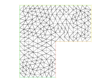
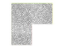
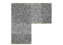
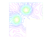
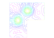
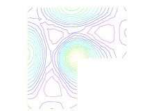
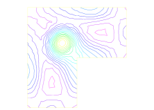
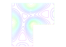
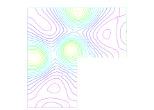
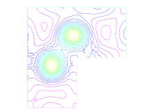
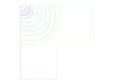
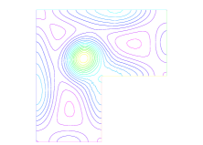
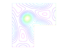
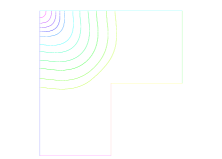
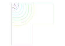
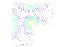
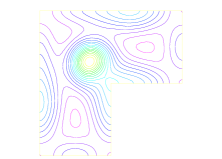
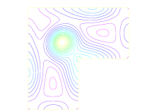
Example 3.1 Firstly, we simulate the the vortex dynamics in an L-shape domain whose longest side has unit length, centered at the origin, with , and
The L-shape domain is triangulated quasi-uniformly, as shown in Figure 4, with nodes per unit length on each side, and we denote by for simplicity.
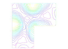
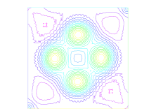
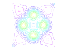
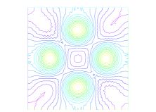
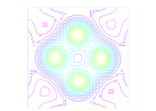
We solve (2.3)-(2.13) with the proposed numerical scheme with piecewise linear finite elements and , and compare the numerical results of the numerical solutions of (1.7)-(1.11) and (1.12)-(1.16), respectively, by using the same finite element mesh and time-step size. The contours of the numerical solutions of are presented in Figure 4–11 with , and . One can see that the numerical solution of (1.7)-(1.11) changes much as the mesh is refined from to ; the numerical solution of (1.12)-(1.16) and (2.3)-(2.13) are relatively stable as the mesh is refined. When or the contours of the three numerical solutions are very different, while when the the numerical solutions of (1.7)-(1.11) and (2.3)-(2.13) agree. Based on these numerical results, we see the following interesting phenomenons:
(2) although the numerical solution of (1.12)-(1.16) is stable as the mesh refines, it converges to an incorrect solution;
Athough the system (2.3)-(2.13) is derived from (1.12)-(1.16) and the two systems are equivalent theoretically, they are not equivalent computationally. Clearly, the reformulated system can be solved easily by the FEMs, while the original system requires extra work to overcome its computational difficulty in a domain with reentrant corners.
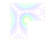
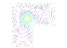
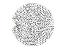
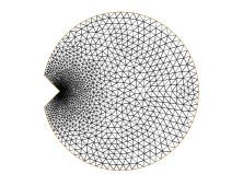
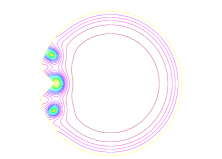
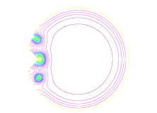
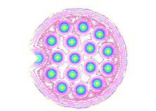
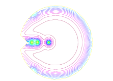
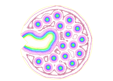
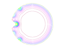
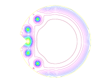
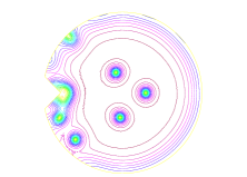
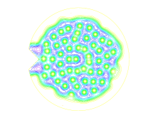
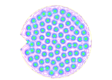
Example 3.2 Secondly, we present simulations of vortex dynamics of a type II superconductor in a circular disk with a triangular defect on the boundary. This example has been tested in [2] with
and with several different values of , by solving the TDGL under the temporal gauge. Details of the geometry of the domain can be found in the reference [2]. Figure 11 contains a quasi-uniform mesh and a locally refined mesh on the circular domain with 64 points on the boundary. Our computations below use similar triangulations with 256 points on the boundary.
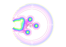
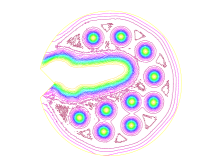
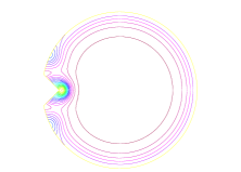
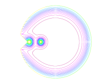
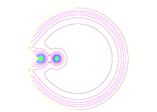
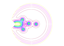
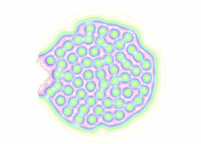
For , we solve (1.7)-(1.11), (1.12)-(1.16) and (2.3)-(2.13), respectively, with and piecewise linear finite elements subject to a quasi-uniform triangulation of the domain with 256 points on the boundary; Figure 11-(a) contains such a triangulation with only 64 points on the boundary. The contours of are presented in Figure 15–15. From Figure 15 one can see that a vortex at the concave corner grows larger and larger as time grows, penetrating into the superconductor, while this giant vortex is not reflected in Figure 15, which we believe is a correct approximation of the exact solution. Excluding the giant vortex at the corner, the rest part of Figure 15 looks similar as Figure 15 when is very large. We believe that the giant vortex is a numerical pollution, whose shape will change if mesh changes (see Figure 15). This indicates that the numerical solution of (1.7)-(1.11) is unstable compared with the numerical solution of (2.3)-(2.13). Clearly, Figure 15 is different from both Figure 15 and Figure 15, and this implies that the finite element solution of (1.12)-(1.16) may converge to an incorrect solution.
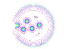
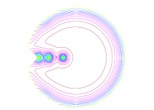
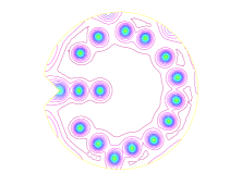
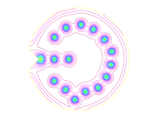
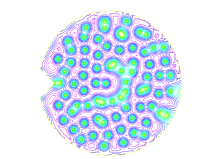
As the external magnetic field grows, the number of vortices increases and the problem becomes more difficult. The numerical results with are present in Figure 19–19. Comparing Figure 19 with Figure 19 we see that, not only a wrong giant vortex may grow at the concave corner when solving (1.7)-(1.11), but many vortices are lost at and near the circular boundary.
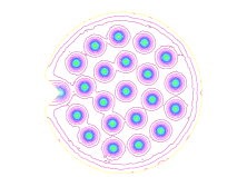
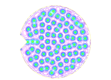
For , there are a larger number of vortices and the problem becomes more difficult. We solve (1.7)-(1.11) and (2.3)-(2.13) with quadratic finite elements subject to a common locally refined mesh; see Figure 11-(b). The numerical results are presented in Figure 19-23, where we see that the numerical solution of the TDGL under the temporal gauge looks strange, while the numerical solution given by our new approach looks reasonable. This shows that our new approach is also superior with locally refined mesh and high-order finite elements.
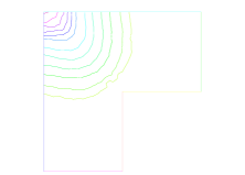
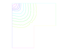
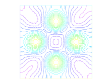
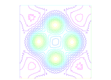
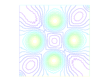
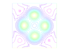
Example 3.3 Finally, we solve the three systems in a convex domain with and
This example was tested before in [6] by solving (1.12)-(1.16), and tested in [29] by solving (1.7)-(1.11). We triangulate the domain into uniform right triangles with 32 points on each side. The contour plots of at different time levels are presented in Figure 23-23 by solving the equations with the time-step size , which show that solving the three systems gives almost the same solution in the domain alway from the corners. Although there is a little difference between Figure 23 and Figure 23-23 near the corners, this difference can be eliminated by using a smaller mesh size. Roughly speaking, the three systems are equivalent in a domain without reentrant corners, both theoretically and computationally.


4. Conclusions
We have introduced a new approach for the numerical simulation of the time-dependent Ginzburg–Landau model of superconductivity in a general curved polygon which may contain reentrant corners, by reformulating the equations under the Lorentz gauge into an equivalent system of equations. Mathematically speaking, this new approach is more suitable for Ginzburg–Landau equations with strong corner singularities. Indeed, numerical simulations demonstrate that it is more stable and accurate than the traditional approaches in the presence of a reentrant corner, and comparably accurate as the traditional approaches in a convex domain.
Acknowledgement. We would like to thank Professor Qiang Du for helpful discussions.
References
- [1] A.A. Abrikosov. Fundamentals of the Theory of Metals. (North-Holland, Amsterdam, 1988).
- [2] T.S. Alstrøm, M.P. Sørensen, N.F. Pedersen, and F. Madsen. Magnetic flux lines in complex geometry type-II superconductors studied by the time dependent Ginzburg–Landau equation. Acta Appl. Math., 115 (2011), pp. 63–74.
- [3] B.J. Baelus, K. Kadowaki, and F.M. Peeters. Influence of surface defects on vortex penetration and expulsion in mesoscopic superconductors. Phys. Rev. B, 71 (2005), 024514
- [4] S. Brenner, J. Cui, Z. Nan, and L.Y. Sung. Hodge decomposition for divergence-free vector fields and two-dimensional Maxwell’s equations. Math. Comp., 81 (2012), pp. 643–659.
- [5] S. Chapman, S. Howison, and J. Ockendon. Macroscopic models for superconductivity. SIAM Review, 34(1992), pp. 529–560.
- [6] Z. Chen and S. Dai. Adaptive Galerkin methods with error control for a dynamical Ginzburg–Landau model in superconductivity. SIAM J. Numer. Anal., 38 (2001), pp. 1961–1985.
- [7] Z. Chen and K.H. Hoffmann. Numerical simulations of dynamical Ginzburg–Landau vortices in superconductivity. In the book Numerical Simulation in Science and Engineering, Notes on Numerical Fluid Mechanics 48 (1994), pp. 31–38.
- [8] Z. Chen, K.H. Hoffmann, and J. Liang. On a non-stationary Ginzburg–Landau superconductivity model. Math. Methods Appl. Sci., 16 (1993), pp. 855–875.
- [9] M. Costabel and M. Dauge. Maxwell and Lamé eigenvalues on polyhedra. Math. Methods Appl. Sci., 22 (1999), pp. 243–258.
- [10] P.G. De Gennes. Superconductivity of Metal and Alloys. Advanced Books Classics, Westview Press, 1999.
- [11] Q. Du, M.D. Gunzburger, and J.S. Peterson. Analysis and approximation of the Ginzburg–Landau model of superconductivity. SIAM Review, 34 (1992), pp. 54–81.
- [12] Q. Du. Global existence and uniqueness of solutions of the time dependent Ginzburg–Landau model for superconductivity, Appl. Anal., 53 (1994), pp. 1–17.
- [13] Q. Du. Numerical approximations of the Ginzburg–Landau models for superconductivity. J. Math. Phys., 46 (2005), 095109.
- [14] H. Frahm, S. Ullah, and A. Dorsey. Flux dynamics and the growth of the superconducting phase. Phys. Rev. Letters, 66 (1991), pp. 3067–3072.
- [15] H. Gao, B. Li, and W. Sun. Optimal error estimates of linearized Crank–Nicolson–Galerkin FEMs for the time-dependent Ginzburg–Landau equations. SIAM J. Numer. Anal., 52 (2014), pp. 1183–1202.
- [16] V. Ginzburg and L. Landau. Theory of Superconductivity. Zh. Eksp. Teor. Fiz., 20 (1950), pp. 1064–1082.
- [17] W.D. Gropp, H.G. Kaper, G.K. Leaf, D.M. Levine, M. Palumbo, and V.M. Vinokur. Numerical simulation of vortex dynamics in type-II superconductors. J. Comput. Phys., 123 (1996), pp. 254–266.
- [18] L.P. Gor’kov and G.M. Eliashberg. Generalization of the Ginzburg–Landau equations for non-stationary problems in the case of alloys with paramagnetic impurities. Soviet Phys. JETP, 27 (1968), pp. 328–334.
- [19] D. Gunter, H. Kaper, and G. Leaf. Implicit integration of the time-dependent Ginzburg–Landau equations of superconductivity. SIAM J. Sci. Comput., 23 (2002), pp. 1943–1958.
- [20] B. Li and Z. Zhang. Mathematical and numerical analysis of time-dependent Ginzburg–Landau equations in nonconvex polygons based on Hodge decomposition. http://arxiv.org/abs/1410.3547
- [21] F. Liu, M. Mondello, and N. Goldenfeld. Kinetics of the superconducting transition. Phys. Rev. Letters, 66 (1991), pp. 3071–3074.
- [22] M. Mu. A linearized Crank–Nicolson–Galerkin method for the Ginzburg–Landau model. SIAM J. Sci. Comput., 18 (1997), pp. 1028–1039.
- [23] M. Mu and Y. Huang. An alternating Crank–Nicolson method for decoupling the Ginzburg–Landau equations, SIAM J. Numer. Anal., 35 (1998), pp. 1740–1761.
- [24] A. Schmid. A time dependent Ginzburg–Landau equation and its application to a problem of resistivity in the mixed state. Phys. kondens. Materie, 5 (1966), pp. 302–317.
- [25] M. Tinkham. Introduction to Superconductivity. 2nd ed., McGraw-Hill, New York, 1994.
- [26] W. Richardson, A. Pardhanani, G. Carey, and A. Ardelea. Numerical effects in the simulation of Ginzburg–Landau models for superconductivity. Int. J. Numer. Engng., 59 (2004), pp. 1251–1272.
- [27] D.Y. Vodolazov, I.L. Maksimov, and E.H. Brandt. Vortex entry conditions in type-II superconductors. Effect of surface defects. Physica C, 384 (2003), pp. 211–226.
- [28] T. Winiecki and C. Adams. A fast semi-implicit finite difference method for the TDGL equation. J. Comput. Phys., 179 (2002), pp. 127–139.
- [29] C. Yang. A linearized Crank–Nicolson–Galerkin FEM for the time-dependent Ginzburg–Landau equations under the temporal gauge. Numerical Methods for Partial Differential Equations, DOI 10.1002/num.21869.