Spin Density Matrix of the $\omega$ in the Reaction ${\bar{p}p}\,\rightarrow\,\omega\pi^{0}$

Abstract

The spin density matrix of the $\omega$ has been determined for the reaction ${\bar{p}p}\,\rightarrow\,\omega\pi^{0}$ with unpolarized in-flight data measured by the Crystal Barrel LEAR experiment at CERN. The two main decay modes of the $\omega$ into $\pi^{0}\gamma$ and $\pi^{+}\pi^{-}\pi^{0}$ have been separately analyzed for various ${\bar{p}}$ momenta between 600 and 1940 MeV/c. The results obtained with the usual method by extracting the matrix elements via the $\omega$ decay angular distributions and with the more sophisticated method via a full partial wave analysis are in good agreement. A strong spin alignment of the $\omega$ is clearly visible in this energy regime and all individual spin density matrix elements exhibit an oscillatory dependence on the production angle. In addition, the largest contributing orbital angular momentum of the ${\bar{p}p}$ system has been identified for the different beam momenta. It increases from $L^{max}_{{\bar{p}p}}$ = 2 at 600 MeV/c to $L^{max}_{{\bar{p}p}}$ = 5 at 1940 MeV/c.

1 Introduction

The spin density matrix of particles originating from ${\bar{p}p}$ annihilations provides important information about the underlying production process. The knowledge of this property is quite scarce in the low energy regime for ${\bar{p}p}$ in-flight reactions and is, however, very fundamental for high quality and high statistics future experiments like PANDA Lutz:2009ff . One major physics topic of PANDA is the spectroscopy of exotic and non-exotic states in the charmonium and open charm mass regions in ${\bar{p}p}$ production or formation processes. For the identification of such resonances it is very helpful to know which initial ${\bar{p}p}$ states contribute and in particular how the corresponding production mechanism can be described in detail. The information about the contributing orbital angular momenta of the initial ${\bar{p}p}$ system and about the spin alignment of vector mesons produced in such processes is therefore an excellent key to gain a deeper insight into the production mechanisms. Therefore the investigation of the reaction ${\bar{p}p}\,\rightarrow\,\omega\pi^{0}$ with a relatively simple final state and without complex decay trees via intermediate resonances provides an excellent access to these questions. The $\omega\pi^{0}$ state couples only to isospin I = 1 and the C-parity C = -1 of the ${\bar{p}p}$ system.

The data presented here have been measured with the Crystal Barrel experiment at LEAR in the years 1995 and 1996. A partial wave analysis has been performed with the PAWIAN software (Partial Wave Interactive Analysis Software) Kopf:2013zz by making use of the helicity formalism and considering the complete reaction chain. Various beam momenta have been studied between 600 and 1940 MeV/c and for two different $\omega$ decay modes, $\omega\,\rightarrow\,\pi^{0}\gamma$ and $\omega\,\rightarrow\,\pi^{+}\pi^{-}\pi^{0}$ , respectively. For the neutral decay mode the polarization of the radiative photon has not been measured and thus it is needed to average over this property.

Similar studies of this reaction for the charged decay mode of the $\omega$ have already been published in Anisovich:2002su . The results presented in the following rely on a more accurate data selection and a refined analysis. First preliminary results for the charged decay mode have already been presented in Kopf:2013zz .

2 Crystal Barrel Experiment

The Crystal Barrel detector, which has been described in detail elsewhere Aker:1992ny , has been designed with a cylindrical geometry along the beam axis. The ${\bar{p}p}$ annihilation took place in a liquid hydrogen target cell with a length of 4.4 cm and a diameter of 1.6 cm located in the center of the detector. This target was surrounded by a silicon vertex detector. This inner part was surrounded by a jet drift chamber which covered 90 % and 64 % of the full solid angle for the inner and outer layer, respectively. These devices together with a solenoid magnet providing a homogeneous 1.5 T magnetic field parallel to the incident beam guaranteed a good vertex reconstruction, tracking and identification for charged particles. For accurate measurements of photons the detector was equipped with a barrel of 1380 CsI(Tl) crystals covering the full azimuthal range of 360^∘ and polar angles from 12^∘ to 168^∘. With this electromagnetic calorimeter, assembled between the jet drift chamber and the solenoid magnet, an energy resolution of $\sigma_{E}/E\approx$ 2.5 % and an angular resolution of 1.2^∘ in $\theta$ and $\phi$ each have been achieved.

3 Data selection and measured angular distributions

The data for this analysis have been taken over various beam times in the years 1995 and 1996 using an unpolarized ${\bar{p}}$-beam and an unpolarized liquid hydrogen target. In most cases the data samples have been recorded by utilizing a 0-prong trigger for the neutral and a 2-prong trigger for the charged decay mode. In addition, a mixed trigger has been used where events with exactly 0 and 2 detected charged particles have been accumulated.

The offline reconstruction and event selection have been performed similarly to the ${\bar{p}p}$ annihilation at rest data Amsler:1993kg . In addition neural networks have been applied for the recognition of misleadingly reconstructed photons induced from electromagnetic Degener:1995xq and hadronic Berlich:1997qj split-offs in the calorimeter. Only exclusive events are considered where all final state particles have been detected. In order to simply reduce the data samples to a more manageable size, preselection cuts have been carried out as follows: exact number of charged particles and photons in the final state and conservation of the total energy ($\Delta E^{tot}\,=\,|E^{tot}_{{\bar{p}p}}-E^{tot}_{rec}|\,<$ 500 MeV) and momentum ($\Delta p^{tot}\,=\,|p^{tot}_{{\bar{p}p}}-p^{tot}_{rec}|\,<$ 500 MeV/c) for the desired reaction. In addition exactly one $\pi^{+}\pi^{-}$ pair must be reconstructed for the charged decay mode originating from a common vertex which is required to be within the target cell. After that kinematic fits with the hypotheses ${\bar{p}p}$$\,\rightarrow\,$$\,\pi^{+}\pi^{-}4\gamma$, $\pi^{+}\pi^{-}2\pi^{0}$, $\omega 2\gamma$ for the charged decay mode and ${\bar{p}p}$$\,\rightarrow\,$$\,5\gamma$, $\pi^{0}\pi^{0}\gamma$, $\omega 2\gamma$ for the neutral decay mode have been performed. Each individual fit requires the conservation of the momentum and energy of the events (4 constraints) and additional constraints on the $\pi^{0}$-mass. Due to the fact that even with these fits the width of the reconstructed invariant mass of the $\omega$ is still dominated by the detector resolution further improvements of the quality of the data has been achieved by constraining the narrow mass of this vector meson (7-constraint fit: ${\bar{p}p}$$\,\rightarrow\,$$\omega\pi^{0}$). It is required that the fit converges with a confidence level (CL) greater than 10 % for each hypothesis. For all beam momenta the distribution of the confidence level is nearly flat and the distributions of the individual pulls are found to be Gaussian centered at 0 with a width of about $\sigma\approx$ 1. This is an indication for a good data quality and for a proper adjusted error matrix. As an example Fig. 1 shows these distributions for the neutral decay mode at 900 MeV/c.

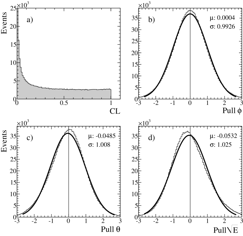
Figure 1: Confidence level and pulls resulting from the kinematic fit for the hypothesis ${\bar{p}p}$$\,\rightarrow\,$$\pi^{0}\pi^{0}\gamma$ performed on the all neutral events at 900 MeV/c beam momentum. The flat distribution of the confidence level (a) and the parameters of the Gaussian fit (black lines) to the pull distribution of the angles $\phi$ and $\theta$ ( (b) and (c) ) and the square root of the energy (d) of the reconstructed photons are indications for the good data quality and for a well understood error matrix. The big enhancement at low confidence level values are caused by background and not properly reconstructed events.

3.1 Signal-background separation

The background contamination is caused by a variety of different sources. One scenario is that channels decaying to slightly different combinations of final state particles contribute where one particle remains undetected or energy deposits in the electromagnetic calorimeter originating from split-off effects are misinterpreted as an additional photon. Another possibility for the fulfillment of all selection criteria is that even channels containing the same final state particles can contribute as background due to misleadingly combined decay products.

For the neutral channel the Dalitz plot of the selected $\pi^{0}\pi^{0}\gamma$ events sheds light on the most crucial background source (Fig. 2). Besides the clear $\omega$ signal, structures from background events are visible whose major origin has been identified as the channel ${\bar{p}p}$$\,\rightarrow\,$$\mathrm{f_{2}(1270)}\,\pi^{0}\,\rightarrow\,(\pi^{0}\pi^{0})\,\pi^{0}\,\rightarrow\,6\gamma$ where one photon remains undetected. In this case the most problematic events are those which appear in the crossing regions of the signal and background band. Due to the fact that in this region the events are located in the same phase space volume it is impossible to reject the background by just applying the selection criteria as described above. Moreover these inhomogeneities of the background events along the $\omega$ band whose distribution is directly correlated to the one of the $\omega$ decay angle would result in huge systematic uncertainties for the determination of the spin density matrix. Since the positions of the crossing regions vary with the incident beam momentum, this situation becomes even more problematic.

Figure 2: Dalitz plots for the selected $\pi^{0}\pi^{0}\gamma$ events at the ${\bar{p}}$ momentum of 900 MeV/c (a) and 1940 MeV/c (b). The $\omega$ signal is visible as strong narrow bands parallel to the horizontal and vertical axis at $\approx$ 6$\cdot\mathrm{10^{5}\,MeV^{2}/c^{4}}$. The remaining bands mainly originate from the $f_{2}(1270)\,\pi^{0}$ background channel. The cross regions between the $\omega$ and the background bands are marked by white ellipses. The comparison between the two plots clearly demonstrates that the positions of the crossing regions strongly depend on the incident beam momentum.

In order to separate these non-interfering background sources from the signal events, an elaborated technique has been used where a signal weight factor Q has been assigned to each event. The strategy has been described in detail in Williams:2009jinst and was successfully applied on CLAS data for the reaction $\gamma\,p\,\rightarrow\,p\,\omega$ Williams:2009ab ; Williams:2009aa . Usual separation methods like the side-band subtraction method are based on the requirement of a binned data set. This exhibits disadvantages due to the complexity in a high dimensional phase space. Instead, the advantages of the technique used here is that it is an event based method and that detailed information about the specific background sources is not needed.

The method takes advantage of the fact that all non-interfering background events cannot reproduce the narrow resonance shape of the $\omega$ meson in the corresponding invariant mass spectrum. Therefore not the fitted $\omega\pi^{0}$ events but rather all selected and fitted $\pi^{0}\pi^{0}\gamma$ events for the neutral and $\pi^{+}\pi^{-}\pi^{0}\pi^{0}$ events for the charged decay mode appearing within a certain window around the relevant $\omega$-mass shape (see Fig. 3b, 4b) are considered for the determination of the Q-value. The procedure starts with the assignment of the nearest neighbors for each event by defining a metric with the relevant kinematic observables. For the neutral channel the metric has been defined via three observables: the polar angle of the $\omega$ production in the ${\bar{p}p}$ rest frame and the azimuth and polar angle of the $\omega$ decay in its helicity system, in which the y-axis is defined to be parallel to the normal vector of the production plane. A subset of 200 neighbors for each event has been chosen which ensures that the associated events cover only a small region of the phase space. A Q value for each event is then obtained by the determination of the signal to background ratio in the invariant mass spectrum of the corresponding data subset. For this an unbinned fit has been performed with a convolution of a Gaussian and a non-relativistic Breit-Wigner function for the description of the $\omega$ signal and a linear approximation for the background content. This approximation can be justified by the assumption that the background events are homogeneously distributed within the small region of the phase space. One example of this fit procedure is illustrated in Fig. 3a. The invariant $\pi^{0}\gamma$ spectrum (Fig. 3b) shows the excellent result for the global signal-background separation obtained for the beam momentum at 900 MeV/c. With the outcome of this approach the final data set for the input of the partial wave analysis has been selected with the fitted $\omega\pi^{0}$ events, each weighted with the corresponding Q-factor.

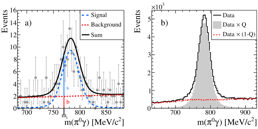
Figure 3: a) Invariant $\pi^{0}\gamma$ mass from a data subset of the 200 nearest neighbors associated to a certain $\pi^{0}\pi^{0}\gamma$ event at the beam momentum of 900 MeV/c. The black shape represents the complete fit result for the determination of the event weight. The dashed blue line shows the obtained content of the $\omega$ signal and the red dotted line the fraction of the background contribution. b) Invariant $\pi^{0}\gamma$ mass of all selected $\pi^{0}\pi^{0}\gamma$ events at 900 MeV/c. The shaded area represents the signal fraction where each event is weighted by its Q-value. The background content with the individual event weight of (1-Q) is marked with the dotted red line.

The same event weight method has been performed for the charged decay mode. Here, the non-interfering background events exhibit as well different shapes in the invariant $\pi^{+}\pi^{-}\pi^{0}$ mass distribution in comparison to the $\omega$ signal. Potential interfering background sources are channels decaying into the same final state particles and can be estimated from the ${\bar{p}p}$ annihilation into the four charged pion final state Bertin:1997vf , i.e.

$$\begin{array}[]{@{}l}{\bar{p}p}\,\rightarrow\,\rho^{+}\rho^{-}\,\rightarrow\,(\pi^{+}\pi^{0})\,(\pi^{-}\pi^{0}),\\ {\bar{p}p}\,\rightarrow\,\rho^{0}f_{2}(1270)\,\rightarrow\,(\pi^{+}\pi^{-})\,(\pi^{0}\pi^{0}),\\ {\bar{p}p}\,\rightarrow\,a_{2}(1320)^{\pm}\pi^{\mp}\,\rightarrow\,(\rho\pi)^{\pm}\pi^{\mp}\,\rightarrow\,(\pi^{\pm}\pi^{0}\pi^{0})\,\pi^{\mp}\quad\mathrm{and}\\ {\bar{p}p}\,\rightarrow\,\eta\pi^{0}\,\rightarrow\,(\pi^{+}\pi^{-}\pi^{0})\,\pi^{0}.\end{array}$$

Due to kinematic reasons these events do not overlap with the $\omega\pi^{0}$ events in the phase-space volume and thus do not contribute to the background. Also the small fraction of combinatorial background of these events do not interfere with the $\omega\pi^{0}$ channel and can therefore be eliminated by the Q-weight method. For the charged decay mode the metric has been defined with four independent observables: the polar angle of the $\omega$ production in the ${\bar{p}p}$ rest frame, the azimuth and polar angle of the normal of the $\omega$ decay plane in its helicity system and the transition rate $\lambda$ of the $\omega$ decay, which is characterized by the cross product of two pion momenta in the $\omega$ helicity frame Williams:2009ab ; Zemach:1964 ; Weidenauer:1993mv :

$$\lambda\, = \,|\mathrm{\vec{p}}_{\pi^{+}}\,\times\,\mathrm{\vec{p}}_{\pi^{-}}|^{2}\,/\,\lambda_{max}$$ (1)

$$\mathrm{with}\quad\lambda_{max} = T^{2}\left(\frac{T^{2}}{108\,c^{4}}+\frac{m_{\pi}T}{9\,c^{2}}+\frac{m_{\pi}^{2}}{3}\right),$$ (2)

$$T = T_{\pi^{+}}+T_{\pi^{-}}+T_{\pi^{0}},$$ (3)

where $T_{\pi}$ represents the kinetic energy of the individual pions. Figure 4 shows very impressively the obtained background separation power. Especially the shape of the normalized transition rate $\lambda$ demonstrates the proper distinction between signal and background events. While the signal events follow the expected $\lambda$-shape for the $\omega$ decay with a linear increase and an intersection at the origin of the axis (0 at $\lambda$=0) the background results in an almost flat distribution.

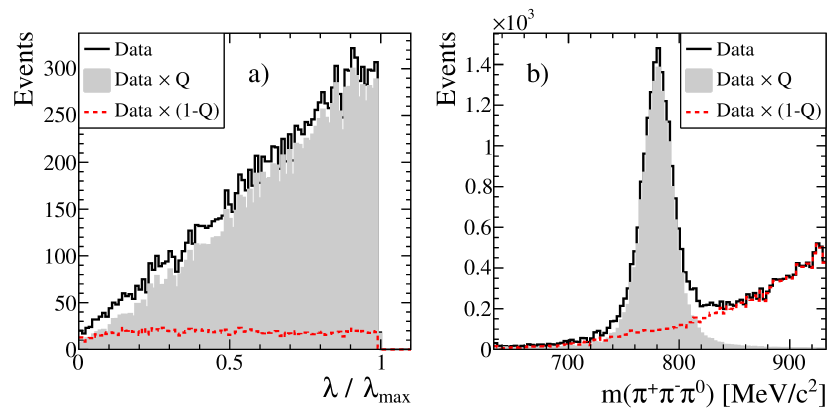
Figure 4: Histogram (a) shows the normalized transition rate $\lambda/\lambda_{max}$ of the $\omega$ decay. Histogram (b) represents the invariant $\pi^{+}\pi^{-}\pi^{0}$ mass of all selected $\pi^{+}\pi^{-}2\pi^{0}$ events at the beam momentum of 900 MeV/c. The excellent background separation power can be seen by the shaded areas representing the fraction of the signal events and the dotted red lines illustrating the background content.

3.2 Overview of the selected data samples

Tables 1 and 2 summarize the numbers of the selected $\omega\pi^{0}$ events without and with the obtained weight factor Q for both decay modes. The number of $\omega\pi^{0}$ signal events is found to be between 1 698 at 1 525 MeV/c and 12 823 at 900 MeV/c for the charged decay mode and between 1 113 at 600 MeV/c and 53 788 at 900 MeV/c for the neutral decay mode, respectively. The large variations of the ratio between the event numbers of the two decay modes for the different beam momenta are mainly caused by the use of different trigger configurations during the data taking. The final data sets consist of sufficient numbers of events for achieving significant results for the partial wave analysis and in particular for the determination of the spin density matrix of the $\omega$. The background contamination estimated by the weight factor (1-Q) depends slightly on the beam momentum and on the decay pattern and varies between 9.2 % and 14.6 % for the charged and 13.7 % and 21.4 % for the neutral decay mode.

Table 1: Used data samples and number of selected events for the channel $\bar{p}p\rightarrow\omega\pi^{0}\rightarrow(\pi^{+}\pi^{-}\pi^{0})\pi^{0}$.

$\bar{p}$ momentum	total number	selected	signal events
$[$MeV/c$]$	of events	$\omega\pi^{0}$ events	$\sum Q$
900	14 890 812	14 460	12 823
1 525	19 591 826	1 871	1 698
1 642	9 371 307	3 475	3 137
1 940	55 814 567	10 942	9 714

Table 2: Used data samples and number of selected events for the channel $\bar{p}p\rightarrow\omega\pi^{0}\rightarrow(\pi^{0}\gamma)\pi^{0}$.

$\bar{p}$ momentum	total number	selected	signal events
$[$MeV/c$]$	of events	$\omega\pi^{0}$ events	$\sum Q$
600	1 046 484	1 369	1 113
900	12 628 286	62 357	53 788
1 050	6 198 731	38 715	33 236
1 350	9 102 322	31 617	25 933
1 525	24 854 889	30 276	24 980
1 642	3 435 070	11 993	9 926
1 800	5 237 105	19 482	15 763
1 940	55 814 567	14 204	11 169

3.3 Measured angular and $\lambda$-distributions

Fig. 5 and Fig. 6 show the relevant angular distributions obtained from the $\omega\pi^{0}$ data after applying all selection and background rejection criteria for the neutral and charged decay mode, respectively. The distributions of the $\omega$ production angle are integrated over the $\omega$-decay distributions and are characterized by fluctuations of the intensity with a higher number of extrema for increased beam momenta. This is an indication that more waves contribute with the rise of the center of mass energy. The huge error bars and the absence of entries around $\left|\,\cos(\theta^{{\bar{p}p}}_{\omega})\,\right|$ = 1 are caused by the acceptance leakage of the detector in the very forward and backward region. These inefficiencies are more distinctive for the charged decay mode due to the limited angular coverage of the tracking devices and become even more apparent with increasing beam momentum. The distributions of the $\omega$-decay angles are integrated over all production angles and exhibit typical shapes for this particle (see Sec. 5).

For all beam momenta the normalized $\lambda$-distributions for the $\omega$-decay to $\pi^{+}\pi^{-}\pi^{0}$ (Fig. 6) are in excellent agreement with the expected shape. This illustrates again the high purity of the $\omega\pi^{0}$ data for the individual beam momenta.

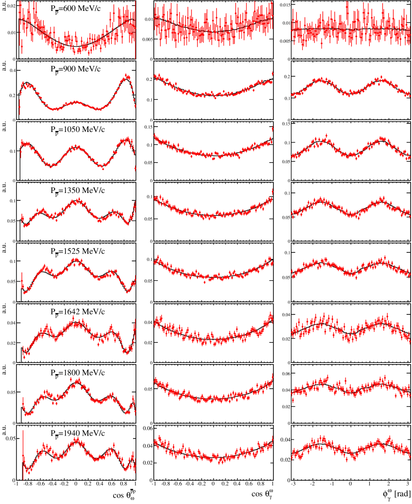
Figure 5: Acceptance corrected angular distributions for the channel ${\bar{p}p}\,\rightarrow\,\omega\pi^{0}$$\,\rightarrow\,$$(\pi^{0}\gamma)\pi^{0}$ as a function of the production angle (first column) and of the decay angle in cos($\theta^{\omega}_{\gamma}$) (second column) and $\phi^{\omega}_{\gamma}$ (third column). The production angle is defined in the ${\bar{p}p}$ rest frame by the direction of the $\omega$ related to the beam axis. The decay angles are specified by the helicity system of the $\omega$ meson. The production angle distribution is given integrated over all $\omega$-decay angles, the decay angle distributions are given integrated over all production angles. While the data are marked with red error bars, the fit results (Sec. 4) are plotted with black lines. Each row represents one specific beam momentum.

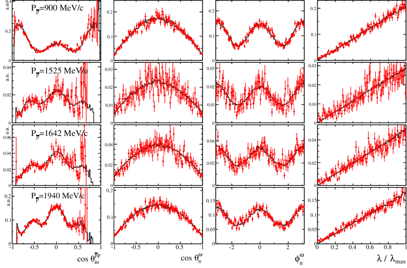
Figure 6: Acceptance corrected angular distributions for the channel ${\bar{p}p}\,\rightarrow\,\omega\pi^{0}$$\,\rightarrow\,$$(\pi^{+}\pi^{-}\pi^{0})\pi^{0}$ as a function of the production angle cos($\theta^{{\bar{p}p}}_{\omega}$) (first column) and of the decay angle in cos($\theta^{\omega}_{n}$) (second column) and $\phi^{\omega}_{n}$ (third column). The production angle is defined in the ${\bar{p}p}$ rest frame by the direction of the $\omega$ related to the beam axis. The decay angles $\theta^{\omega}_{n}$ and $\phi^{\omega}_{n}$ are specified by the normal of the decay plane of the $\omega$ meson in its helicity system. The production angular distribution is integrated over all $\omega$-decay angles, the decay angular distributions are integrated over all production angles. The fourth column represents the normalized transition rate $\lambda$ of the $\omega$ decay. A detailed description of this property can be found in sec. 3.1. While the data are marked with red error bars, the fit results (Sec. 4) are plotted with black lines. Each row represents one specific beam momentum.

4 Partial wave analysis

4.1 Amplitudes

${\bar{p}p}$ in-flight reactions where mesons and photons are exclusively involved are dominated by the s-channel process. Therefore the partial wave analyses for those reactions have been started usually with the $J^{PC}$ system initiated from the ${\bar{p}p}$ annihilation. One difficulty of this method is that additional Clebsch-Gordan coefficients for the coupling of the ${\bar{p}p}$ system with the $J^{PC}$ intermediate state are not considered correctly. In order to avoid such error-prone procedure, the analysis performed on the data here is based on the description of the complete reaction chain starting from the ${\bar{p}p}$ coupling up to the final states. This new method is summarized in detail in HKoch:2012 and can also be applied to other ${\bar{p}p}$ reactions in flight.

The starting point is the description of the differential cross section of the whole reaction chain where the transition amplitude depending on the helicities of the involved particles is divided into the $\omega$-production and the $\omega$-decay amplitude. For the neutral channel this cross section is expressed by

$$\frac{d\sigma}{d\tau}\propto w\,=\,\sum_{\scriptsize\begin{array}[]{@{}l}\lambda_{\bar{p}},\lambda_{p},\lambda_{\pi^{0}_{r}}(=0),\\ \lambda_{\pi^{0}_{d}}(=0),\lambda_{\gamma}\end{array}}\Big{|}\sum_{\lambda_{\omega}} T_{\lambda_{\bar{p}}\lambda_{p}\lambda_{\pi^{0}_{r}}\lambda_{\omega}}^{{\bar{p}p}\rightarrow\omega\pi^{0}_{r}}(cos(\theta^{\bar{p}p}_{\omega}))$$ (6)

$$\cdot A_{\lambda_{\omega}\lambda_{\pi^{0}_{d}}\lambda_{\gamma}}^{\omega\rightarrow\pi^{0}_{d}\gamma}(cos(\theta^{\omega}_{\gamma}),\phi^{\omega}_{\gamma})\Big{|}^{2},$$ (7)

where $d\tau$ represents the infinitesimal volume element of the phase-space, $w$ the transition probability, $\lambda$ the helicities of all involved particles, $T$ the production and $A$ the decay amplitude in the helicity frame. The two neutral pions are distinguished by the notation $\pi^{0}_{r}$ for the recoil particle and $\pi^{0}_{d}$ for the $\omega$ decay particle. Due to the fact that a mass constraint for the $\omega$ has been used for the kinematic fit the dynamics for this meson (e.g. a Breit-Wigner distribution) has not been taken into account. It is noteworthy to mention that the components of the transition amplitude are added coherently over the helicities of the intermediate $\omega$- resonance and incoherently over the helicities of all initial and final state particles. Eq. 6 is expanded into states with definite $J^{PC}$-values defining the partial wave helicity amplitudes $T^{J^{PC}}_{\lambda_{{\bar{p}}},\lambda_{p},0,\lambda_{\omega}}$ and $A^{1^{--}}_{\lambda_{\omega}\lambda_{\gamma}}$. These partial wave amplitudes are further expanded in states with definite $J^{PC}$, $L$, $S$-values where $L,S$ are the respective orbital angular momenta and total spins of the ${\bar{p}p}$, $\omega\pi^{0}$ and $\pi^{0}\gamma$-system ($L_{{\bar{p}p}}$, $S_{{\bar{p}p}}$, $L_{\omega\pi^{0}}$, $S_{\omega\pi^{0}}$(=1), $L_{\pi^{0}\gamma}$(=1), $S_{\pi^{0}\gamma}$(=1)), defining the amplitudes $T_{L_{{\bar{p}p}},S_{{\bar{p}p}},L_{\omega\pi^{0}}}^{J_{{\bar{p}p}}}$ and $A_{L_{\pi^{0}\gamma},S_{\pi^{0}\gamma}}^{1}=A^{1}_{11}$. Here, the quantum number $J$ represents the total angular momentum, $L$ the orbital angular momentum and $S$ the total spin of the related system composed of two particles. The underlying formalism for theses expansions can be found in detail elsewhere Chung:1971ri . With the requirement that the parity, charge conjugation and total angular momentum are conserved for strong and electromagnetic interactions the differential cross section can be described by incoherent sums over the ${\bar{p}p}$ singlet and triplet states and over the helicity of the radiative photon of the final state system HKoch:2012 . In terms of $LS$-amplitudes Eq. 6 reads HKoch:2012 :

$$w = \sum_{\lambda_{\gamma},\lambda_{p},\,\lambda_{{\bar{p}}}}\Big{|}\sum_{J_{\bar{p}p}}\sum_{L_{\bar{p}p},S_{\bar{p}p}}\sum_{L_{\omega\pi^{0}},\lambda_{\omega}}\,\sqrt{2L_{\bar{p}p}+1}$$ (8)

$$\cdot\langle L_{\bar{p}p},0,S_{\bar{p}p},M_{\bar{p}p}|J_{{\bar{p}p}},M_{{\bar{p}p}}\rangle\,\langle\frac{1}{2},\lambda_{\bar{p}},\frac{1}{2},-\lambda_{p}|S_{{\bar{p}p}},M_{{\bar{p}p}}\rangle$$

$$\cdot\sqrt{2L_{\omega\pi^{0}}+1}\,\langle L_{\omega\pi^{0}},0,1,\lambda_{\omega}|J_{{\bar{p}p}},\lambda_{\omega}\rangle\,d^{J_{{\bar{p}p}}}_{M_{{\bar{p}p}}\,\lambda_{\omega}}(\theta^{{\bar{p}p}}_{\omega})$$

$$\cdot T_{L_{{\bar{p}p}},S_{{\bar{p}p}},L_{\omega\pi^{0}}}^{J_{{\bar{p}p}}}\,\cdot\,\sqrt{\frac{3}{8\pi}}$$

$$\cdot\,D^{1*}_{\lambda_{\omega}\lambda_{\gamma}}(\theta^{\omega}_{\gamma},\phi^{\omega}_{\gamma})\cdot A_{11}^{1}\cdot\lambda_{\gamma}\Big{|}^{2},$$

with $M_{{\bar{p}p}}=\lambda_{\bar{p}}-\lambda_{p}$. The summation over $\lambda_{\bar{p}}$ and $\lambda_{p}$ can be arranged in such a way, that one incoherent term for singlet states ($S_{{\bar{p}p}}=0,M_{{\bar{p}p}}=0$) and three incoherent terms for triplet states ($S_{{\bar{p}p}}=1,M_{{\bar{p}p}}=0,\pm 1$) appear. The direction of the ${\bar{p}}$ beam is chosen as the quantization axis which results in the restriction of the z-component of $J_{{\bar{p}p}}$ to $M_{{\bar{p}p}}=0,\pm 1$. The $\omega\pi^{0}$ system is fully characterized by $L_{\omega\pi^{0}}$, $S_{\omega\pi^{0}}$=1, the helicity $\lambda_{\omega}$ and the production angle $\theta_{\omega}^{{\bar{p}p}}$ of the $\omega$ in the ${\bar{p}p}$ rest frame. Due to the fact that the ${\bar{p}p}$ system is unpolarized the angle $\phi_{\omega}^{{\bar{p}p}}$ is not defined. The $\omega$ decay system is characterized by the angular momentum $L_{\pi^{0}_{d}\gamma}$=1, the total spin $S_{\pi^{0}_{d}\gamma}$=1, the helicity $\lambda_{\gamma}$ and the decay angles $\theta_{\gamma}^{\omega}$ and $\phi_{\gamma}^{\omega}$ of the $\gamma$ in the helicity frame of the $\omega$ meson. The $d_{M_{\bar{p}p},\lambda_{\omega}}^{J_{\bar{p}p}}$ denotes the Wigner-d function for the decay of the ${\bar{p}p}$ system, $D_{\lambda_{\omega},\lambda_{\gamma}}^{*J_{\omega}=1}$ the complex conjugate of the Wigner-D function for the $\omega$ decay and $\langle L,0,S,\lambda_{1}-\lambda_{2}|J,\lambda_{1}-\lambda_{2}\rangle$ and $\langle j_{1},\lambda_{1},j_{2},-\lambda_{2}|S,\lambda_{1}-\lambda_{2}\rangle$ the Clebsch-Gordan coefficients for the $LS$- and $jj$-coupling respectively. As $A^{1}_{11}$ for a given ${\bar{p}p}$-energy is a fixed complex number, the product $T_{L_{{\bar{p}p}},S_{{\bar{p}p}},L_{\omega\pi^{0}}}^{J_{{\bar{p}p}}}\cdot A^{1}_{11}$ is handled as one complex parameter $\alpha^{J^{PC}}_{L_{{\bar{p}p}}L_{\omega{\pi^{0}}}}$.

For the reaction ${\bar{p}p}\,\rightarrow\,\omega\pi^{0}$ $\rightarrow\,(\pi^{+}\pi^{-}\pi^{0})\,\pi^{0}$ Eq. 8 has to be modified Chung:1971ri . The incoherent sum over $\lambda_{\gamma}$ vanishes and the $\omega$ decay amplitude $A^{1^{--}}_{\lambda_{\omega}\lambda_{\gamma}}$ has to be replaced by

$$\sqrt{\frac{3}{4\pi}}\cdot D^{1*}_{\lambda_{\omega}\mu}(\Theta^{\omega}_{n},\Phi^{\omega}_{n},\gamma^{\omega}_{n})\cdot A^{1}_{\mu}(E_{\pi^{+}},E_{\pi^{-}}),$$ (9)

where $\Theta^{\omega}_{n},\Phi^{\omega}_{n},\gamma^{\omega}_{n}$ are the Euler angles of the normal of the $3\pi$-decay plane ($\vec{n}$) in the $\omega$-helicity system with $\mu=\langle\vec{J}_{\omega}\cdot\vec{n}\rangle$. In general $\mu$ takes the values $\pm 1,0$, but in the $\omega\rightarrow\pi^{+}\pi^{-}\pi^{0}$ case, only $\mu=0$ is allowed. $A^{1}_{\mu}(E_{\pi^{+}},E_{\pi^{-}})$ describes the amplitude in the Dalitz plot, which is proportional to $|\vec{P}_{\pi^{+}}\times\vec{P}_{\pi^{-}}|$ Zemach:1964 .

By making use of the conservation principles and the selection rules one can easily extract the specific combinations of the relevant quantum numbers allowed for the reaction ${\bar{p}p}\,\rightarrow\,\omega\pi^{0}$ (Tab. 3).

Table 3: Combinations of the allowed quantum numbers for the reaction ${\bar{p}p}\,\rightarrow\,\omega\pi^{0}$. The $J^{PC}$ combinations even^+- and odd^-+ are forbidden for the ${\bar{p}p}$ system and the combinations even^-+, even⁺⁺ and odd⁺⁺ are not allowed for the $\omega\pi^{0}$ coupling. The quantum numbers for the $\omega$ decay to $\pi^{0}\gamma$ ( $L_{\pi^{0}\gamma}$=1, $S_{\pi^{0}\gamma}$=1 ) and to $\pi^{+}\pi^{-}\pi^{0}$ ( $L_{\pi^{+}\pi^{-}\pi^{0}}$=1, $S_{\pi^{+}\pi^{-}\pi^{0}}$=0 ) and $S_{\omega\pi^{0}}$=1 for the $\omega\pi^{0}$ coupling are not given explicitly.

$J^{PC}$	$L_{\bar{p}p}$	$S_{\bar{p}p}$	$M_{\bar{p}p}$	$L_{\omega\pi^{0}}$
0–	not allowed for ${\bar{p}p}$ reaction
even–	J	1	$\pm$1	J-1, J+1
odd–	J-1, J+1	1	0 ,$\pm$1	J
odd+-	J	0	0	J-1, J+1

4.2 Fits to data and determination of the parameters $\alpha$

Unbinned maximum likelihood fits were performed for each beam momentum and decay mode individually in order to determine the best hypothesis with the resulting fit parameters $\alpha^{J^{PC}}_{L_{{\bar{p}p}}L_{\omega\pi^{0}}}$. Input for this method are the selected data with the obtained event weights $Q_{i}$ as well as phase-space distributed Monte Carlo events. For properly taking into account the detector resolution and acceptance the GEANT3 transport code has been used. To considering also the correct reconstruction efficiency these Monte Carlo events were then undergoing the same reconstruction and selection criteria as applied for data events and described in section 3. The extended likelihood function $\mathcal{L}$ is defined as SBischoff:1999 :

$$\mathcal{L}\propto n_{data}!\cdot\exp\Big{(}-\frac{(n_{data}-\overline{n})^{2}}{2n_{data}}\Big{)}\cdot\prod_{i=1}^{n_{data}}\frac{w(\vec{\tau_{i}},\vec{\alpha})\,\epsilon(\vec{\tau_{i}})}{\int w(\vec{\tau},\vec{\alpha})\,\epsilon(\vec{\tau})\,\mathrm{d}\tau}$$

where $n_{data}$ denotes the number of data events, $\vec{\tau}$ the phase-space coordinates, $\vec{\alpha}$ the complex fit parameter, $\epsilon(\vec{\tau})$ the acceptance and reconstruction efficiency at the position $\vec{\tau}$ and $\overline{n}=n_{data}\cdot\int w(\vec{\tau},\vec{\alpha})\,\epsilon(\vec{\tau})\,\mathrm{d}\tau/\int\epsilon(\tau)\,\mathrm{d}\tau$. The $w(\vec{\tau},\vec{\alpha})$ represents the transition probability given by Eq. 8. By logarithmizing Eq. 4.2, approximating the integrals with Monte Carlo events and introducing the weight $Q_{i}$ for each event, the final function to be minimized is then given by:

$$-\ln\,\mathcal{L} \approx -\sum_{i=1}^{n_{data}}\ln(w(\vec{\tau_{i}},\vec{\alpha})\cdot Q_{i})$$ (11)

$$+\Big{(}\sum_{i=1}^{n_{data}}Q_{i}\Big{)}\,\cdot\,\ln\Big{(}\frac{\sum_{j=1}^{n_{MC}}w(\vec{\tau_{j}},\vec{\alpha})}{n_{MC}}\Big{)}$$

$$+\frac{1}{2}\,\cdot\,\Big{(}\sum_{i=1}^{n_{data}}Q_{i}\Big{)}\,\cdot\,\Big{(}\frac{\sum_{j=1}^{n_{MC}}w(\vec{\tau_{j}},\vec{\alpha})}{n_{MC}}-1\Big{)}^{2},$$

where $n_{MC}$ represents the number of selected Monte Carlo events.

To obtain the best hypothesis for the description of the data a strategy has been carried out where fits with successive increase of the maximal contributing orbital angular momentum $L^{max}_{{\bar{p}p}}$ have been performed. For each of those fits all allowed waves with $L_{{\bar{p}p}}\leq L^{max}_{{\bar{p}p}}$ have been taken into account. The fit results have been compared using the likelihood ratio. With this strategy it was feasible to determine unambiguously the best hypothesis and thus the largest contributing orbital angular momentum $L^{max}_{{\bar{p}p}}$ for all data samples. Summaries of the obtained results are listed in Tab. 4 and Tab. 5, respectively. Except for the beam momentum of 1525 MeV/c the results for the charged and neutral decay modes are consistent. The slight discrepancy for only one beam momentum is likely caused by the limited acceptance of the detector for the charged decay mode and thus the results for the neutral decay mode are more reliable. For the initial states $J^{PC}=even^{--}$ and $J^{PC}=odd^{+-}$ two different orbital angular momenta $L_{\omega\pi^{0}}=J-1$ and $L_{\omega\pi^{0}}=J+1$ for the $\omega\pi^{0}$-system are possible (see Tab. 3) . It turned out that for all fits both waves for this system contribute. As an example the fit result with the obtained parameter values are summarized in Tab. 6 for the charged decay mode at the beam momentum of 900 MeV/c.

The maximal contributing orbital angular momentum $L_{\bar{p}p}^{max}$ increases continuously from 2 at the lowest beam momentum of 600 MeV/c up to 5 at the highest beam momentum of 1940 MeV/c. These values are in good agreement with a former analysis Abele:2000qq . Partial wave annihilation cross sections as a function of the ${\bar{p}}$ beam momentum for several $L_{\bar{p}p}$ values have been estimated Mundigl:1991jp ; Weise:1993py . Figure 7 shows the outcome of these model calculations for a typical hadronic radius of the baryon core of $\langle r_{B}^{2}\rangle^{1/2}\,=\,0.6\,fm$. Under this assumption the minimum ${\bar{p}}$-beam momentum for the production of $L_{\bar{p}p}=3$ states is expected to be roughly 0.7 GeV, for $L_{\bar{p}p}=4,5$ states it is expected to be 1.0 and 1.5  GeV, respectively. The results presented here are in good agreement with these model calculations and only differ in slightly lower momentum thresholds.

Table 4: Best fit results for $L^{max}_{{\bar{p}p}}$ for the channel ${\bar{p}p}\,\rightarrow\,\omega\pi^{0}$$\,\rightarrow\,$($\pi^{+}\pi^{-}\pi^{0}$) $\pi^{0}$. The significant improvement in comparison to the hypothesis with $L_{\bar{p}p}^{max}-1$ and the marginal improvement of the assumption with $L_{\bar{p}p}^{max}+1$ is a good indication for the unambiguousness of the fit result. The significance is denoted in units of the standard deviation $\sigma$.

momentum	$L_{\bar{p}p}^{max}$	significance of likelihood ratio
$[$MeV/c$]$		$\frac{\ln L(L_{\bar{p}p}^{max})}{\ln L(L_{\bar{p}p}^{max}-1)}$	$\frac{\ln L(L_{\bar{p}p}^{max}+1)}{\ln L(L_{\bar{p}p}^{max})}$
900	4	2.2 $\sigma$	0.13 $\sigma$
1525	4	9.0 $\sigma$	0.90 $\sigma$
1642	5	3.2 $\sigma$	0.06 $\sigma$
1940	5	>10 $\sigma$	1.04 $\sigma$

Table 5: Best fit results for $L_{\bar{p}p}^{max}$ for the channel ${\bar{p}p}\,\rightarrow\,\omega\pi^{0}$$\,\rightarrow\,$$(\pi^{0}\gamma)\pi^{0}$. For further explanations see the caption of Tab. 4.

momentum	$L_{\bar{p}p}^{max}$	significance of likelihood ratio
$[$MeV/c$]$		$\frac{\ln L(L_{\bar{p}p}^{max})}{\ln L(L_{\bar{p}p}^{max}-1)}$	$\frac{\ln L(L_{\bar{p}p}^{max}+1)}{\ln L(L_{\bar{p}p}^{max})}$
600	2	>10 $\sigma$	1.05 $\sigma$
900	4	6.5 $\sigma$	0.22 $\sigma$
1050	4	>10 $\sigma$	0.01 $\sigma$
1350	5	5.6 $\sigma$	0.03 $\sigma$
1525	5	>10 $\sigma$	0.25 $\sigma$
1642	5	5.0 $\sigma$	8$\cdot$10${}^{-3}\,\sigma$
1800	5	>10 $\sigma$	0.55 $\sigma$
1940	5	>10 $\sigma$	0.69 $\sigma$

Table 6: Fitted parameters for the reaction ${\bar{p}p}\,\rightarrow\,\omega\pi^{0}$ $\rightarrow\,(\pi^{+}\pi^{-}\pi^{0})\,\pi^{0}$ at 900 MeV/c beam momentum and $L^{max}_{{\bar{p}p}}=4$. The L,S correspond to the $\overline{p}p$, $\omega\pi^{0}$ or $\omega$ system, respectively. For technical reasons the $\alpha^{J^{PC}}_{L_{{\bar{p}p}}L_{\omega\pi^{0}}}$ were split into two parameters where some can be fixed due to the linear dependency. Furthermore, two additional phases can be fixed as only relative phases are relevant. The errors are statistical only and originated from the covariance matrix obtained by the fit.

Parameter for $J^{PC}\,(L,S)$	Magnitude	Phase
$\overline{p}p\ \mathrm{system}$
$1^{--}\,(0,1)$	0.4 $\pm$ 0.04	0 (fixed)
$1^{--}\,(2,1)$	0.13 $\pm$ 0.08	1.8 $\pm$ 0.4
$1^{+-}\,(1,0)$	0.36 $\pm$ 0.03	0 (fixed)
$2^{--}\,(2,1)$	0.20 $\pm$ 0.04	-2.86 $\pm$ 0.19
$3^{--}\,(2,1)$	0.16 $\pm$ 0.06	1.49 $\pm$ 0.27
$3^{--}\,(4,1)$	0.15 $\pm$ 0.06	1.47 $\pm$ 0.24
$3^{+-}\,(3,0)$	0.190 $\pm$ 0.028	2.09 $\pm$ 0.19
$4^{--}\,(4,1)$	0.135 $\pm$ 0.016	0.9 $\pm$ 0.3
$5^{--}\,(4,1)$	0.08 $\pm$ 0.04	1.9 $\pm$ 0.5
$\omega\pi^{0}$ production
$1^{--}\,(1,1)$	1 (fixed)	0 (fixed)
$1^{+-}\,(0,1)$	0.70710 (fixed)	0 (fixed)
$1^{+-}\,(2,1)$	0.62 $\pm$ 0.15	1.20 $\pm$ 0.17
$2^{--}\,(1,1)$	0.70710 (fixed)	0 (fixed)
$2^{--}\,(3,1)$	0.85 $\pm$ 0.14	0.71 $\pm$ 0.28
$3^{--}\,(3,1)$	1 (fixed)	0 (fixed)
$3^{+-}\,(2,1)$	0.70710 (fixed)	0 (fixed)
$3^{+-}\,(4,1)$	0.85 $\pm$ 0.11	0.22 $\pm$ 0.24
$4^{--}\,(3,1)$	0.70710 (fixed)	0 (fixed)
$4^{--}\,(5,1)$	0.8 $\pm$ 0.1	0.69 $\pm$ 0.16
$5^{--}\,(5,1)$	1 (fixed)	0 (fixed)
$\omega$ decay
$1^{--}\,(1,0)$	1(fixed)	0 (fixed)

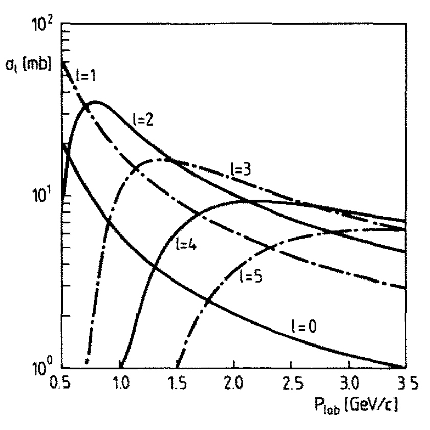
Figure 7: Estimated partial wave annihilation cross sections as a function of the ${\bar{p}}$ beam momentum for several $L_{\bar{p}p}$ based on model calculations Mundigl:1991jp ; Weise:1993py . The main input parameter for this model is the nucleon radius, which is assumed to be $\langle r_{B}^{2}\rangle^{1/2}\,=\,0.6\,fm$. This figure is extracted from Mundigl:1991jp .

4.3 Comparison of data and fits

The fitted $\omega$-production and $\omega$-decay angles and the normalized $\lambda$-value (in case of the charged $\omega$-decay) are compared with the data in Fig. 5 and Fig. 6. Apart from minor systematic discrepancies the agreement is good. The reasonable description of the data can also be seen in the fit quality summarized in Tab. 7. The goodness-of-fit has been estimated with the Pearson $\chi^{2}$ test based on the histograms for the relevant kinematic variables (Fig. 5 and Fig. 6) by calculating

$$\frac{\chi^{2}}{ndf}=\sum_{i=1}^{n}\sum_{j=1}^{N_{bins,i}}\Big{(}\frac{(\nu_{ij,fit}-\nu_{ij,data})^{2}}{\nu_{ij,data}}\Big{)}/(N_{bins}-N_{params}),$$ (12)

where n represents the number of the relevant kinematic variables, $N_{bins,i}$ the number of bins for the histogram $i$,$\nu_{ij,data/fit}$ the number of data/fit entries within bin $j$ for the histogram $i$ and $N_{params}$ the number of fit parameters. The $\chi^{2}$ values divided by the number of degrees of freedom vary between 0.82 and 1.36 which are reasonable results. However, one has to remark that Eq. 12 does not consider the correlations between the different kinematic variables and thus only serves as a rough estimate for the fit quality.

Table 7: Fit quality $\chi^{2}/ndf$ for the charged and neutral decay mode obtained with the Pearson $\chi^{2}$ test.

momentum	$\chi^{2}/ndf\;(ndf)$
$[$MeV/c$]$	$\omega$$\,\rightarrow\,$$\pi^{+}\pi^{-}\pi^{0}$	$\omega$$\,\rightarrow\,$$\pi^{0}\gamma$
600	–	0.82 (282)
900	1.16 (371)	1.36 (274)
1050	–	1.18 (273)
1350	–	1.04 (268)
1525	1.13 (356)	1.13 (268)
1642	1.04 (352)	1.27 (267)
1800	–	1.21 (267)
1940	1.02 (351)	1.20 (267)

5 Spin density matrix of the $\omega$

In addition to the contributing orbital momenta, the polarization observables of the $\omega$ meson exhibit important information about its production process. These properties are in general defined by spherical momentum tensors or alternatively by the spin density matrix $\rho$, which is used in the following. Since the $\omega$ is a particle with spin 1 its spin density matrix contains 3x3 complex elements $\rho_{\lambda_{i}\lambda_{j}}$, where $\lambda_{i}$ and $\lambda_{j}$ represent the helicities of the $\omega$-particle. The $\rho$-matrix is hermitian with a trace of 1 by definition. Polarization means $\rho_{11}\neq\rho_{-1-1}$ and alignment is defined as $\rho_{11}=\rho_{-1-1}\neq\rho_{00}$. For measurements with unpolarized protons and antiprotons for channels where the parity is conserved and by choosing the quantization axis to be in the production plane, the number of independent $\rho$-elements is reduced to four real quantities. The $\omega$ spin density matrix for the reaction ${\bar{p}p}\,\rightarrow\,\omega\pi^{0}$ is given by Schilling:1969um :

$$\rho=\left(\begin{array}[]{ccc}1/2(1-\rho_{00})&\Re\rho_{10}+i\Im\rho_{10}&\rho_{1-1}\\ \Re\rho_{10}-i\Im\rho_{10}&\rho_{00}&-\Re\rho_{10}+i\Im\rho_{10}\\ \rho_{1-1}&-\Re\rho_{10}-i\Im\rho_{10}&1/2(1-\rho_{00})\end{array}\right)$$ (16)

The $\rho$-matrix elements are dependent on the quantization axis which is here chosen to be the one of the $\omega$-helicity system defined by the $\omega$ flight direction in the ${\bar{p}p}$ center of mass system. The helicity system is the most suitable one to use for this kind of ${\bar{p}p}$ reactions which is strongly dominated by the s-channel process. In addition, the elements are dependent on the center of mass energy and on the production angle.

The determination of the $\omega$-matrix elements has been performed by two different methods: (1) by using the results of the partial wave analysis and (2) solely via the angular decay distributions of the $\omega$-meson. The first method is very rarely used and has already been applied successfully for the reaction $\gamma\mathrm{p}\,\rightarrow\,\mathrm{p}\omega$  Williams:2009aa . It uses the fitted production amplitude, here defined as $T_{\lambda_{\bar{p}}\lambda_{p}\lambda_{\pi^{0}_{r}}\lambda_{\omega}}({\bar{p}p}\,\rightarrow\,\omega\pi^{0})$ (Sec. 4), which contains the information of the $\omega$ spin density matrix. The individual $\rho$-elements can be extracted from the production amplitude by Kutschke:1996 :

$$\rho_{\lambda_{i}\lambda_{j}}=\frac{1}{N}\sum_{\lambda_{{\bar{p}}},\lambda_{p},\lambda_{\pi^{0}_{r}}=0}T_{\lambda_{\bar{p}}\lambda_{p}\lambda_{\pi^{0}_{r}}\lambda_{i}}^{*}T_{\lambda_{\bar{p}}\lambda_{p}\lambda_{\pi^{0}_{r}}\lambda_{j}},$$ (18)

where $N$ is the normalization factor:

$$N=\sum_{\lambda_{{\bar{p}}},\lambda_{p},\lambda_{\omega},\lambda_{\pi^{0}_{r}}=0}|T_{\lambda_{\bar{p}}\lambda_{p}\lambda_{\pi^{0}_{r}}\lambda_{\omega}}|^{2}$$ (19)

According to Eq. 18 the $\rho$-matrix elements have been projected out from the production amplitude obtained from the partial wave fit of the full reaction chain. In our case (unpolarized initial states) the differential cross section is only dependent on $\rho_{00}$, $\rho_{1-1}$ and $\Re\rho_{10}$, so that only these matrix elements can be extracted. The results as function of the center of mass energy and the $\omega$-production angle are summarized in Fig. 8 and 9. The statistical errors have been calculated by propagating the covariance matrix obtained by the likelihood fit. Additionally, a much more time consuming bootstrap approach as described in Vernarsky:2014 has been tested which yielded results that are in full agreement to the first calculation.

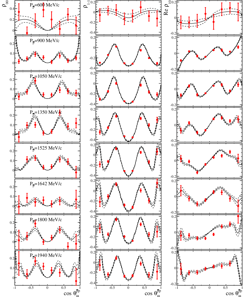
Figure 8: Spin density matrix elements $\rho_{00}$ (first column), $\rho_{1-1}$ (second column) and $\rho_{10}$ (third column) of the $\omega$ in its helicity frame as function of the production angle for the reaction ${\bar{p}p}\,\rightarrow\,\omega\pi^{0}$$\,\rightarrow\,$$(\pi^{0}\gamma)\pi^{0}$. While the results obtained via the $\omega$-decay angles are marked with red error bars, the outcome via the partial wave analysis is plotted with continuous black lines. The dashed black lines represent the statistical errors of the partial wave result. Each row represents one specific beam momentum.

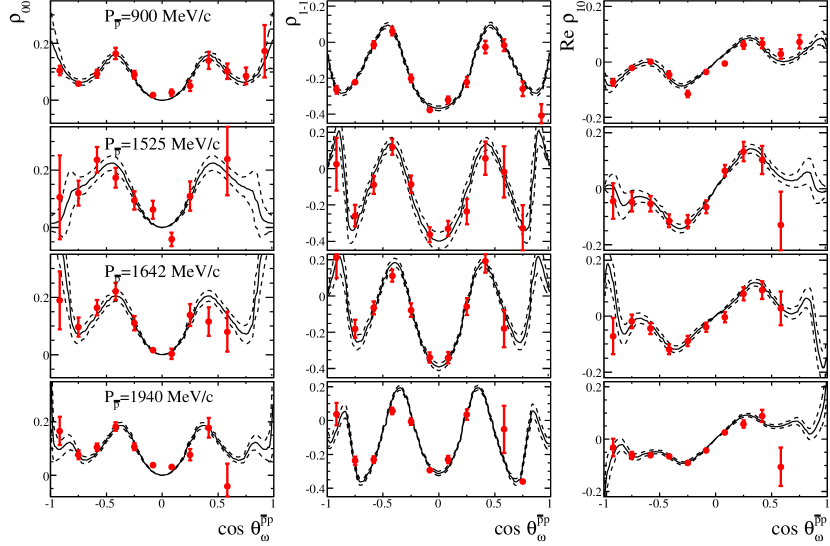
Figure 9: Spin density matrix elements $\rho_{00}$ (first column), $\rho_{1-1}$ (second column) and $\rho_{10}$ (third column) of the $\omega$ in its helicity frame as function of the production angle for the reaction ${\bar{p}p}\,\rightarrow\,\omega\pi^{0}$$\,\rightarrow\,$$(\pi^{+}\pi^{-}\pi^{0})\pi^{0}$. While the results obtained via the $\omega$-decay angles are marked with red error bars, the outcome via the partial wave analysis is plotted with continuous black lines. The dashed black lines represent the statistical errors of the partial wave result. Each row represents one specific beam momentum.

The second and more traditional method, also calledSchilling method, does not make use of the results of the partial wave analysis and uses only the distribution of the $\omega$ decay angles $\theta$ and $\phi$ Schilling:1969um . The angular distribution for the charged decay mode is given by:

$$W(\theta^{\omega}_{n},\phi^{\omega}_{n}) = \frac{3}{4\pi}\sum_{\lambda_{\omega}\lambda_{\omega}^{\prime}}\,D^{*1}_{\lambda_{\omega}0}(\theta^{\omega}_{n},\phi^{\omega}_{n})\,\rho_{\lambda_{\omega}\lambda_{\omega}^{\prime}}\,D^{1}_{\lambda_{\omega}^{\prime}0}(\theta^{\omega}_{n},\phi^{\omega}_{n})$$ (20)

$$= \frac{3}{4\pi}\,\Big{(}\frac{1}{2}\,(1-\rho_{00})\,+\,\frac{1}{2}\,(3\rho_{00}-1)\,\cos^{2}\theta^{\omega}_{n}$$

$$-\sqrt{2}\,\Re\rho_{10}\,\sin 2\theta^{\omega}_{n}\,\cos\phi^{\omega}_{n}$$

$$-\rho_{1-1}\,\sin^{2}\theta^{\omega}_{n}\,\cos 2\phi^{\omega}_{n}\Big{)},$$

and for the neutral decay mode by:

$$W(\theta^{\omega}_{\gamma},\phi^{\omega}_{\gamma}) = \frac{3}{4\pi}\sum_{\lambda_{\omega}\lambda_{\omega}^{\prime}\lambda_{\gamma}}D^{*1}_{\lambda_{\omega}\lambda_{\gamma}}(\theta^{\omega}_{\gamma},\phi^{\omega}_{\gamma})\rho_{\lambda_{\omega}\lambda_{\omega}^{\prime}}D^{1}_{\lambda_{\omega}^{\prime}\lambda_{\gamma}}(\theta^{\omega}_{\gamma},\phi^{\omega}_{\gamma})$$ (21)

$$= \frac{3}{4\pi}\Big{(}\frac{1}{2}\,(1-\rho_{00})\,+\,\frac{1}{2}\,(1-3\rho_{00})\,\cos^{2}\theta^{\omega}_{\gamma}$$

$$+\,\sqrt{2}\,\Re\rho_{10}\,\sin 2\theta^{\omega}_{\gamma}\,\cos\phi^{\omega}_{\gamma}$$

$$+\,\rho_{1-1}\,\sin^{2}\theta^{\omega}_{\gamma}\,\cos 2\phi^{\omega}_{\gamma}\Big{)}$$

As can be seen from Eq. 20 and 21 only the elements of the real part of the matrix are sensitive to the $\omega$ decay angular distribution, which are $\rho_{00}$, $\rho_{1-1}$ and $\Re\rho_{10}$. The imaginary part $\Im\rho_{10}$ related to an eventual $\omega$-polarization perpendicular to the scattering plane is not accessible. The matrix elements have been extracted separately for different bins in the production angle by fitting the two dimensional $\omega$ decay distribution according to Eq. 20 for the charged decay mode and Eq. 21 for the neutral decay mode with a maximum likelihood fit procedure analogous to the one described before in sec. 4.2. While the two methods rely on different approaches, both, however, should yield the same results. Due to the fact that binned data in the production angle are needed for the Schilling method the determination of the $\rho$-matrix elements with this method is not as accurate as for the first one which naturally imposes all the physical constraints and correlations.

The good agreement between the results obtained with the two different methods can clearly be seen in Fig. 8 for the neutral decay mode and in Fig. 9 for the charged decay mode. It is noticeable that in case of the PWA method the statistical errors are smaller in comparison to the Schilling method. The $\rho$-matrix elements show a strong oscillatory dependence on the $\omega$-production angle cos($\theta^{\bar{p}p}_{\omega}$). The $\rho_{00}$ and $\rho_{1-1}$ have minima and maxima for $\cos(\theta^{\bar{p}p}_{\omega})=0$ and $|\cos(\theta^{\bar{p}p}_{\omega})|=0.4$, respectively. The $\rho_{00}$-values averaged over the production angle are listed in Tab. 8. These values show a clear spin alignment effect ($\rho_{00}=1/3$ would correspond to no spin-alignment).

Table 8: $\rho_{00}$-values of the $\omega$ meson averaged over the production angle. The averaging is limited on the range of the production angle with a reasonable detector acceptance, which is between $-0.85\leq\cos\theta^{\bar{p}p}_{\omega}\leq 0.4$ for the charged and $-0.85\leq\cos\theta^{\bar{p}p}_{\omega}\leq 0.95$ for the neutral decay mode. Only the statistical errors are listed below. The systematic errors are not considered here.

momentum	$\overline{\rho_{00}}$
$[$MeV/c$]$	$\omega\rightarrow\pi^{+}\pi^{-}\pi^{0}$	$\omega\rightarrow\pi^{0}\gamma$
	($-0.85\leq\cos\theta^{\omega}_{n}\leq 0.4$)	($-0.85\leq\cos\theta^{\omega}_{\gamma}\leq 0.95$)
600	-	0.15 $\pm$ 0.05
900	0.069 $\pm$ 0.008	0.047 $\pm$ 0.008
1050	-	0.064 $\pm$ 0.011
1350	-	0.075 $\pm$ 0.012
1525	0.106 $\pm$ 0.016	0.065 $\pm$ 0.009
1642	0.094 $\pm$ 0.013	0.028 $\pm$ 0.012
1800	-	0.060 $\pm$ 0.013
1940	0.083 $\pm$ 0.007	0.060 $\pm$ 0.015

The results for the charged and the corresponding neutral decay mode are in an overall good agreement for all beam momenta. However, differences are visible which are in particular strongly depending on the production angle. These inconsistencies are more significant for the results obtained with the PWA method due to the relatively small statistical errors and might be caused by systematic uncertainties in the simulation and reconstruction procedure.

Similar dependencies on the production angle have already been observed for the tensor polarisation observables of the $\omega$ in the same reaction ${\bar{p}p}\,\rightarrow\,\omega\pi^{0}$ Anisovich:2002su . In addition the values obtained in the analysis here can be compared with earlier vector meson production experiments in ${\bar{p}p}$-interactions at higher energies. Also there explicit alignment effects for the $\rho$-meson have been observed Lednicky:1983 . This is in contrast to $pp$-reactions, where negligible alignment for $\rho^{0}$ is reported Blobel:1973wr . This trend is also observed in low energy pp-reactions for the orientation of the $\omega$-spin AbdelBary:2010er .

6 Summary

The reaction ${\bar{p}p}\,\rightarrow\,\omega\pi^{0}$ with unpolarized in-flight data has been analyzed in detail. The $\omega$ meson with the neutral decay to $\pi^{0}\gamma$ as well as with the charged decay to $\pi^{+}\pi^{-}\pi^{0}$ has been investigated separately in the low energy regime for various ${\bar{p}}$ beam momenta between 600 and 1940 MeV/c. An excellent background rejection power has been achieved by determining an event based signal weight factor. The performed partial wave analysis has taken into account the complete reaction chain starting from the ${\bar{p}p}$ coupling up to the final state particles. It described the data with high precision. The maximal contributing orbital angular momentum $L^{max}_{\bar{p}p}$ increases continuously from 2 at the lowest beam momentum of 600 MeV/c up to 5 at the highest beam momentum of 1940 MeV/c. The elements of the spin density matrix have been determined with two different methods. The results based on the outcome of the partial wave analysis and those based on the $\omega$ decay distributions are in excellent agreement. The first method via the production amplitudes of the PWA was only used in a few cases up to now. The individual elements exhibit a strong dependency on the $\omega$-production angle. A clear spin alignment with $\rho_{00}$ values between 0% and 25% over the whole angular range within $|\cos(\theta)|\,<\,$0.9 is visible.

References

- (1) M. F. M. Lutz et al. [PANDA Collaboration], arXiv:0903.3905 [hep-ex].
- (2) B. Kopf, H. Koch, J. Pychy and U. Wiedner, Hyperfine Interact. 229, no. 1-3, 69 (2014).
- (3) A. V. Anisovich, C. A. Baker, C. J. Batty, D. V. Bugg, L. Montanet, V. A. Nikonov, A. V. Sarantsev and V. V. Sarantsev et al., Phys. Lett. B 542, 8 (2002) [arXiv:1109.5247 [hep-ex]].
- (4) E. Aker et al. [Crystal Barrel Collaboration], Nucl. Instrum. Meth. A 321, 69 (1992).
- (5) C. Amsler et al. [Crystal Barrel Collaboration], Z. Phys. C 58, 175 (1993).
- (6) T. F. Degener and M. Kunze, Int. J. Mod. Phys. C 6, 599 (1995).
- (7) R. Berlich and M. Kunze, Nucl. Instrum. Meth. A 389, 274 (1997).
- (8) M. Williams and M. Bellis and C. A. Meyer, JINST 4, P10003, (2008).
- (9) M. Williams et al. [CLAS Collaboration], Phys. Rev. C 80, 065208 (2009) [arXiv:0908.2910 [nucl-ex]].
- (10) M. Williams et al. [CLAS Collaboration], Phys. Rev. C 80, 065209 (2009) [arXiv:0908.2911 [nucl-ex]].
- (11) A. Bertin et al. [OBELIX Collaboration], Phys. Lett. B 414, 220 (1997).
- (12) C. Zemach, Phys. Rev. 133 B1201 (1964).
- (13) P. Weidenauer et al. [ASTERIX. Collaboration], Z. Phys. C 59, 387 (1993).
- (14) H. Koch, “Helicity Amplitude for , ", PANDA-Note AN-QCD-2012-001, 2012, “https://lxpndwww.gsi.de/content/documents”, unpublished.
- (15) S. U. Chung, CERN-71-08.
- (16) S. Bischoff, PhD thesis, Universität Karlsruhe, 1999.
- (17) A. Abele et al. [Crystal Barrel Collaboration], Eur. Phys. J. C 12, 429 (2000).
- (18) S. Mundigl, M. J. Vicente Vacas and W. Weise, Nucl. Phys. A 523, 499 (1991).
- (19) W. Weise, Nucl. Phys. A 558, 219C (1993).
- (20) K. Schilling, P. Seyboth and G. E. Wolf, Nucl. Phys. B 15, 397 (1970) [Erratum-ibid. B 18, 332 (1970)].
- (21) R. Kutschke, “An Angular Distribution Cookbook”, 1996, “http://home.fnal.gov/~kutschke/”, unpublished.
- (22) B. Vernarsky, PhD thesis, Carnegie Mellon University, 2014.
- (23) R. Lednicky, Czech. J. Phys. B 33, 1177 (1983).
- (24) V. Blobel et al. [Bonn-Hamburg-Munich Collaboration], Phys. Lett. B 48, 73 (1974).
- (25) M. Abdel-Bary et al. [TOF Collaboration], Eur. Phys. J. A 44, 7 (2010) [arXiv:1001.3043 [nucl-ex]].