On the meson mass spectrum in the covariant confined quark model

Abstract

We provide a new insight into the problem of generating the hadron mass spectrum in the framework of the covariant confined quark model. One of the underlying principles of this model is the compositeness condition which means that the wave function renormalization constant of the elementary hadron is equal to zero. In particular, this equation allows to express the Yukawa coupling of the meson fields to the constituent quarks as a function of other model parameters. In addition to the compositeness condition we also employ a further equation which relates the meson mass function to the Fermi coupling. Both equations guarantee that the Yukawa-type theory is equivalent to the Fermi-type theory thereby providing an interpretation of the meson field as the bound state of its constituent fermions (quarks). We evaluate the Fermi-coupling as a function of meson (pseudoscalar and vector) masses and vary the values of the masses in such a way to obtain a smooth behavior for the resulting curve. The mass spectrum obtained in this manner is found to be in good agreement with the experimental data. We also compare the behavior of our Fermi-coupling with the strong QCD coupling $\alpha_{s}$ calculated in an QCD-inspired approach.

I   Introduction

One of the puzzles of hadron physics is the origin of the hadron masses. The Standard Model (SM) and, in particular, quantum chromodynamics (QCD) operate only with fundamental particles (quarks, leptons, neutrinos), gauge bosons and the Higgs. It is not yet clear how to explain the appearance of the multitude of observed hadrons and elucidate the generation of their masses. Therefore, the calculation of the hadron mass spectrum in a quality comparable to the precision of experimental data still remains one of the major problems in QCD.

Actually, even before QCD was set up as the fundamental theory of strong interactions, it was understood that it is a difficult problem to describe a composite particle within quantum field theory as based on the relativistic S-matrix. The reason is that quantum field theory operates with free fields which are quantized by imposing commutator (anti-commutator) relations between creation and annihilation operators. The asymptotic in- and out-states are constructed by means of these operators acting on the vacuum state. Physical processes are described by the elements of the S-matrix taken for the relevant in- and out-states. In perturbation theory, which originally has a mathematical meaning, the matrix elements are represented by a set of the Feynman diagrams which are the convolution of free Green functions (or propagators). The original Lagrangian describing free fields and their interactions requires renormalization, i.e. the transition from bare or unrenormalized quantities like mass, wave function, coupling constant to the physical or renormalized ones. In particular, the bare field is related to the dressed one by the wave function renormalization constant as $\phi_{0}=Z^{1/2}\phi_{r}$. One can see that the bare field $\phi_{0}$ may be eliminated from the Lagrangian by putting its wave function renormalization constant to be zero, $Z=0$. Probably one of the first who suggested to use the equation $Z=0$ as a compositeness condition was Jouvet Jouvet:1956ii . He showed that the four-fermion theory is equivalent to a Yukawa-type theory if the renormalization constant of the boson field is set to zero. The crucial point in comparison of the two theories is related to the renormalization of the Yukawa-type theory, i.e. the transition from the bare quantities (boson mass, boson wave function, Yukawa coupling) to the physical or renormalized ones. Then the renormalized (experimental) boson mass and Yukawa coupling may be expressed through the Fermi constant via the compositeness condition.

Salam extended the condition of setting the wave function renormalization constant to zero by requiring that the vertex renormalization constant must be equal to zero, too Salam:1962ap . In this way he showed that the obtained theory included the bootstrap idea in quantum field theory. Some aspects of this approach were developed further in Braun:1970df .

Weinberg showed that the compositeness condition $Z=0$ results in a sum rule for the coupling of a composite particle to its constituents as a function of energy Weinberg:1962hj . Further developments and applications of the compositeness condition may be found in a monograph Lurie:1968zz and a review Hayashi:1967hk . We also should mention the work of Anikin:1995cf . There it was shown that the nonlocal Nambu–Jona-Lasinio (NJL) model is equivalent to the Yukawa theory of scalar and pseudoscalar fields interacting with their constituents if the wave function normalization constants are set to zero. Some physical, low-energy observables have been calculated in the framework of this approach.

One of the phenomenological approaches is the model of induced quark currents. It is based on the hypothesis that the QCD vacuum is realized by the  anti-!self-dual homogeneous gluon field Burdanov:1996uw . The confining properties of the vacuum field, chiral symmetry breaking, and the localization of a composite field at the center of mass of the quark bound state can explain the distinctive features of the meson spectrum: mass splitting between pseudoscalar and vector mesons, Regge trajectories and the asymptotic mass formulas in the heavy quark limit. This model describes to within ten percent accuracy the masses and weak decay constants of mesons.

In a series of papers Efimov:2001ng ; Ganbold:2009ak ; Ganbold:2010bu ; Ganbold:2012zz relativistic models with specific forms of analytically confined propagators have been developed to study some aspects of low-energy hadron physics. The role of analytic confinement in the formation of two-particle bound states has been analyzed within a simple Yukawa model of two interacting scalar fields, the prototypes of ’quarks’ and ’gluons’  Efimov:2001ng . The spectra of the’ two-quark’ and ’two-gluon’ bound states have been defined by using master constraints similar to the ladder Bethe-Salpeter equations. The ’scalar confinement’ model could explain semiquantitatively the asymptotically linear Regge trajectories of ’mesonic’ excitations and the existence of massive ’glueball’ states. It has also been shown that physically reasonable bound states could be formed at relatively weak coupling. An extension of this model by introducing color and spin degrees of freedom, different constituent quark masses and the confinement size parameter has been performed in Ganbold:2009ak . Specific forms of analytically confined propagators of quarks and gluons have been used to take into account the correct symmetry structure of the quark-gluon interaction in the confinement region. The masses of conventional mesons have been estimated (with relative errors less than $3.5$ per cent) in a wide energy range. As a further test the calculated weak decay constants of light mesons ($f_{\pi}$ and $f_{K}$) are in good accordance with the experimental data. Additionally, the lowest-state glueball mass has been predicted which is in reasonable agreement with other theoretical approaches. A phenomenological model with infrared-confined propagators has been developed to take into account the dependence of the QCD effective coupling $\alpha_{s}=g^{2}/4\pi$ on the mass scale and to study its behavior at large distances  Ganbold:2012zz . First the pseudoscalar and vector meson masses have been calculated in the region above  2 GeV. By fitting the estimated masses to the recent experimental data model parameters could be fixed, namely the constituent quark masses $m_{f},\{f=u,d,s,c,b\}$ and the value $\Lambda$ of the confinement scale. By fitting the experimental masses of intermediate and light mesons we have predicted the behavior of $\alpha_{s}$ in the low-energy domain. Note, we have also derived analytically a new, specific and finite behavior of $\alpha_{s}(M)$ at the origin $M=0$ that increased by decreasing the value of the confinement scale value. Note that $\alpha_{s}(0)$ depends on $\Lambda$, we fixed $\alpha_{s}(0)=0.757$ for $\Lambda=345$ MeV Ganbold:2010bu and $\alpha_{s}(0)=0.8498$ for $\Lambda=220$ MeV Ganbold:2014zda .

The compositeness condition $Z_{H}=0$ is also one of the key ingredients in the relativistic constituent quark model developed for the first time in Efimov:1988yd (see also the extensive treatment in Efimov:1993ei ). The model has found numerous applications both in the meson sector meson and in baryon physics baryon . In the latter case baryons are considered as relativistic systems composed of three quarks. The next step in the development of the model has been done in Ref. Branz:2009cd where infrared confinement was introduced guaranteeing the absence of all possible thresholds corresponding to quark production. The implementation of quark confinement allowed to use the same values for the constituent quark masses both for the simplest quark-antiquark systems (mesons) and more complicated multiquark configurations (baryons, tetraquarks, etc.). Note that we prefer to name this approach as the covariant quark model which is more appropriate in the context of a comparison with other quark models.

The infrared cutoff parameter $\lambda$ is taken to have a common value for all processes considered. The model parameters (constituent quark masses $m_{q}$, the infrared cutoff parameter $\lambda$ and the size parameters $\Lambda_{H}$ that characterize the distribution of the constituent quarks inside the hadron $H$) have been determined by a fit to available experimental data. The last fit was performed in Ref. Ivanov:2011aa . This approach was successfully applied in the calculation of transition form factors needed to study the semileptonic, nonleptonic and rare decays of the $B$-meson and the $\Lambda_{b}$-baryon B-physics . The X(3872) meson was treated as four-quark state (tetraquark) tetraquark . Its strong and radiative decays have been calculated. For reasonable values of the size parameter of the X(3872) we found consistency with the available experimental data.

It should be emphasized that the experimental values of hadron masses are used in all calculations performed in the covariant quark model. As discussed above, the theory with Yukawa couplings describing the interaction of mesons and their constituent quarks is equivalent to the theory with a four-fermion interaction. This is the case if, first, the wave function renormalization constant of the meson field is equal to zero and, second, the coupling $G$ characterizing the strength of the four-fermion interaction is related to the meson mass function. Up to now we have used the first equation $Z_{H}=1-g^{2}_{r}\tilde{\Pi}^{\prime}(m^{2}_{H})=0$ to determine the renormalized Yukawa coupling $g_{r}$ as a function of meson mass and model parameters. In this paper we are aiming to use also the second equation $G\tilde{\Pi}(m^{2}_{H})=1$ to investigate the dependence of the coupling $G$ on physical meson masses.

The paper is organized in the following way. In Sec.II we give a brief sketch of the approach to the bound state problem in quantum field theory based on the compositeness condition with $Z_{H}=0$. By using the functional integral we demonstrate explicitly that the four-fermion theory with the Fermi coupling $G$ is equivalent to the Yukawa-type theory if, first, the wave function renormalization constant in the Yukawa theory is equal to zero and, second, the Fermi coupling $G$ is inversely proportional to the meson mass function calculated at the physical meson mass. In Sec.III we give the details of the calculation for the mass function of pseudoscalar and vector mesons in the framework of the covariant quark model. In Sec.IV we update the fit of model parameters and calculate the Fermi coupling $G$ as a function of the physical mass in a quite large region ranging from the $\pi$ up to $B_{c}$ mesons. We suggest a smoothness criterion to generate a continuous behavior of the Fermi coupling $G$. The mass spectrum obtained in this manner is found to be in good agreement with the experimental data. We compare the behavior of $G$ with the strong QCD coupling $\alpha_{s}$ calculated in the QCD-inspired approach. Finally, in Sec. IV we summarize our findings.

II   The compositeness condition $Z_{H}=0$

The use of the compositeness condition $Z_{H}=0$ is one of the outstanding approaches to the bound state problem in quantum field theory. Historically, this condition first appeared when looking for the bound state in a four-fermion theory with the Lagrangian

$${\cal L}_{F}=\bar{q}(i\not\!\partial-m_{q})q\,+\,\frac{G}{2}\,\bigl{(}\bar{q}\Gamma q\bigr{)}^{2}\,.$$ (1)

Here, for simplicity, we drop all color and flavor indices. For the general Dirac matrix we use $\Gamma=I,i\gamma^{5}$, i.e. we restrict to bound states with zero spin. We will consider the bound state problem by using the chain (one-loop) approximation but the result is general and can be proved to all orders of perturbation theory. In the following, for simplicity, we will not consider the renormalization of the fermion (“quark”) fields.

The bare Lagrangian with a Yukawa coupling of the boson field $\phi_{0}$ to the fermions is written as

$${\cal L}_{Y}=\bar{q}(i\not\!\partial-m_{q})q\,+\,\frac{1}{2}\phi_{0}(\Box-m^{2}_{0})\phi_{0}+g_{0}\phi_{0}\,\bigl{(}\bar{q}\Gamma q\bigr{)}\,,\quad\text{where}\quad\Box=-\partial^{\mu}\partial_{\mu}\,.$$ (2)

The more transparent way to demonstrate the renormalization procedure is the use of the functional integral. The vacuum generating functional for the Yukawa theory is written as

$$Z_{Y}=\int\!\!{\cal D}\phi_{0}\!\int\!\!{\cal D}\bar{q}\!\int\!\!{\cal D}q\,e^{i\int\!dx{\cal L}_{Y}(x)}\,.$$ (3)

Hereafter, we will drop all irrelevant normalization constants. Integrating out the quark fields

$$\int\!\!{\cal D}\bar{q}\!\int\!\!{\cal D}q\,e^{i\int\!\!dx\!\int\!dy\,\bar{q}(x)\bigl{[}(i\not\!\partial_{x}-m_{q})\delta(x-y)\,+\,\delta(x-y)\,g_{0}\phi_{0}(y)\Gamma\bigr{]}\,q(y)}$$ (4)

$$= {\rm det}||(i\not\!\partial_{x}-m_{q})\delta(x-y)\,+\,\delta(x-y)\,g_{0}\phi_{0}(y)\Gamma||$$

$$\Longrightarrow {\rm det}||\delta(x-y)\,+\,(i\not\!\partial_{x}-m_{q})^{-1}\delta(x-y)\,g_{0}\phi_{0}(y)\Gamma||$$

$$= {\rm det}||\delta(x-y)\,-\,iS_{q}(x-y)g_{0}\phi_{0}(y)\Gamma||$$

$$= \exp\bigl{\{}-\sum_{n=1}^{\infty}\frac{i^{n}}{n}g_{0}^{n}\int\!\!dx_{1}\ldots\!\int\!\!dx_{n}\phi_{0}(x_{1})\ldots\phi_{0}(x_{n})\mbox{\rm{tr}}[\Gamma S_{q}(x_{1}-x_{2})\ldots\Gamma S_{q}(x_{n}-x_{1})]\bigr{\}}.$$

one finds

$$Z_{Y} = \int\!\!{\cal D}\phi_{0}\exp\bigl{\{}\frac{i}{2}\int\!\!dx\phi_{0}(x)(\Box-m^{2}_{0})\phi_{0}(x)$$ (5)

$$- \sum_{n=1}^{\infty}\frac{i^{n}}{n}g_{0}^{n}\int\!\!dx_{1}\ldots\!\int\!\!dx_{n}\phi_{0}(x_{1})\ldots\phi_{0}(x_{n})\mbox{\rm{tr}}[\Gamma S_{q}(x_{1}-x_{2})\ldots\Gamma S_{q}(x_{n}-x_{1})]\bigr{\}}.$$

Here we introduce the quark Green function in the usual form as

$$S_{q}(x-y)=\int\frac{d^{4}k}{(2\pi)^{4}i}\frac{e^{-ik(x-y)}}{m_{q}-\not\!k}\,.$$ (6)

Then we collect the terms bi-linear in the boson fields. One gets

$$L^{(2)}_{Y} = \frac{1}{2}\!\int\!\!dx\,\phi_{0}(x)(\Box-m^{2}_{0})\phi_{0}(x)$$ (7)

$$- \frac{i}{2}\,g_{0}^{2}\!\int\!\!dx_{1}\!\!\int\!\!dx_{2}\phi_{0}(x_{1})\phi_{0}(x_{2})\mbox{\rm{tr}}[\Gamma S_{q}(x_{1}-x_{2})\Gamma S_{q}(x_{2}-x_{1})]$$

$$= \frac{1}{2}\!\int\!\!dx\,\phi_{0}(x)(\Box-m^{2}_{0})\phi_{0}(x)+\frac{1}{2}\,g_{0}^{2}\!\int\!\!dx_{1}\!\!\int\!\!dx_{2}\,\phi_{0}(x_{1})\Pi_{S=0}(x_{1}-x_{2})\phi_{0}(x_{2})$$

where we define the mass function of the boson with spin $S=0$ as

$$\Pi_{S=0}(x_{1}-x_{2})=i\,\langle T\bigl{\{}\bigl{[}\bar{q}\Gamma q\bigr{]}_{x}\bigl{[}\bar{q}\Gamma q\bigr{]}_{y}\bigr{\}}\rangle_{0}=-i\,\mbox{\rm{tr}}[\Gamma S_{q}(x_{1}-x_{2})\Gamma S_{q}(x_{2}-x_{1})]\,.$$ (8)

Expanding the Fourier transform of this mass function at the physical value of the boson mass up to the second order

$$\tilde{\Pi}_{S=0}(p^{2})=\int\!\!dx\,e^{-ipx}\Pi_{S=0}(x)=\tilde{\Pi}_{S=0}(m^{2})+(p^{2}-m^{2})\tilde{\Pi}^{\prime}_{S=0}(m^{2})+\tilde{\Pi}_{S=0}^{\rm ren}(p^{2})$$ (9)

one finds

$$L^{(2)}_{Y} = \frac{1}{2}\!\int\!\!dx\,\phi_{0}(x)(\Box-m^{2}_{0}+g_{0}^{2}\tilde{\Pi}_{S=0}(m^{2})+(\Box-m^{2})\tilde{\Pi}^{\prime}_{S=0}(m^{2}))\phi_{0}(x)$$ (10)

$$+ \frac{1}{2}\,g_{0}^{2}\!\int\!\!dx_{1}\!\!\int\!\!dx_{2}\,\phi_{0}(x_{1})\Pi^{\rm ren}_{S=0}(x_{1}-x_{2})\phi_{0}(x_{2})\,.$$

The renormalization of boson mass, wave function and Yukawa coupling proceed in the standard manner

$$m^{2} = m^{2}_{0}-g_{0}^{2}\,\tilde{\Pi}_{S=0}(m^{2}),\qquad\phi_{r}=Z^{-1/2}\phi_{0},$$

$$g_{r} = Z^{1/2}g_{0},\qquad Z=\frac{1}{1+g_{0}^{2}\,\tilde{\Pi}^{\prime}_{S=0}(m^{2})}\,.$$ (11)

Note that the wave function renormalization constant may be expressed via the renormalized coupling constant

$$Z=1-g_{r}^{2}\,\tilde{\Pi}^{\prime}_{S=0}(m^{2})\,.$$ (12)

Finally, the renormalized generating functional for the Yukawa theory is written as

$$Z^{\rm ren}_{Y} = \int\!\!{\cal D}\phi_{r}\exp\bigl{\{}\frac{i}{2}\int\!\!dx\phi_{r}(x)(\Box-m^{2})\phi_{r}(x)$$ (13)

$$+ \frac{i}{2}\,g_{r}^{2}\!\int\!\!dx_{1}\!\!\int\!\!dx_{2}\,\phi_{r}(x_{1})\Pi^{\rm ren}_{S=0}(x_{1}-x_{2})\phi_{r}(x_{2})$$

$$- \sum_{n=3}^{\infty}\frac{i^{n}}{n}g_{r}^{n}\int\!\!dx_{1}\ldots\!\int\!\!dx_{n}\phi_{r}(x_{1})\ldots\phi_{r}(x_{n})\mbox{\rm{tr}}[\Gamma S_{q}(x_{1}-x_{2})\ldots\Gamma S_{q}(x_{n}-x_{1})]\bigr{\}}\,.$$

We drop the linear boson term because it is absent for pseudoscalar mesons and it can be removed in the scalar case by a shift of the field.

Now we consider the generating functional for the Fermi theory

$$Z_{F}=\int\!\!{\cal D}\bar{q}\!\int\!\!{\cal D}q\,e^{i\int\!dx{\cal L}_{F}(x)}$$ (14)

where the Lagrangian ${\cal L}_{F}(x)$ is given by Eq. (1). By using the Gaussian functional representation for the exponential of the four-fermion interaction

$$e^{i\frac{G}{2}\langle(\bar{q}\Gamma q)^{2}\rangle}=N_{+}^{-1}\int\!\!{\cal D}\phi\exp\{-\frac{i}{2}\frac{1}{G}\langle\phi^{2}\rangle+i\langle\phi\cdot(\bar{q}\Gamma q)\rangle\}\quad\text{where}\quad\langle(...)\rangle=\int\!dx\,(...)$$ (15)

one finds

$$Z_{F}=N_{+}^{-1}\int\!\!{\cal D}\phi\!\int\!\!{\cal D}\bar{q}\!\int\!\!{\cal D}q\,\exp\{-\frac{i}{2}\frac{1}{G}\langle\phi^{2}\rangle\,+\,i\,\langle\bar{q}\bigl{[}i\not\!\partial-m_{q}\,+\,\phi\Gamma\bigr{]}q\rangle\}.$$ (16)

Then we integrate out the quark fields

$$Z_{F} = \int\!\!{\cal D}\phi\exp\bigl{\{}-\frac{i}{2}\frac{1}{G}\int\!dx\,\phi^{2}(x)$$ (17)

$$- \sum_{n=1}^{\infty}\frac{i^{n}}{n}\int\!\!dx_{1}\ldots\!\int\!\!dx_{n}\phi(x_{1})\ldots\phi(x_{n})\mbox{\rm{tr}}[\Gamma S_{q}(x_{1}-x_{2})\ldots\Gamma S_{q}(x_{n}-x_{1})]\bigr{\}}$$

where we drop all irrelevant normalization constants. Next we collect the terms bi-linear in the boson fields and introduce the renormalized mass function like in the Yukawa case. One gets

$$L^{(2)}_{F} = \frac{1}{2}\!\int\!\!dx\,\phi(x)\Big{(}-\frac{1}{G}+\tilde{\Pi}_{S=0}(m^{2})+(\Box-m^{2})\tilde{\Pi}^{\prime}_{S=0}(m^{2})\Big{)}\phi(x)$$ (18)

$$+ \frac{1}{2}\,\int\!\!dx_{1}\!\!\int\!\!dx_{2}\,\phi(x_{1})\Pi^{\rm ren}_{S=0}(x_{1}-x_{2})\phi(x_{2})\,.$$

If we require the condition

$$G\,\tilde{\Pi}_{S=0}(m^{2})=1$$ (19)

and rescale the boson field as $\phi\to\phi/\sqrt{\tilde{\Pi}^{\prime}_{S=0}(m^{2})}$ one obtains the free Lagrangian of the boson field with the mass $m$ and the correct residue of the Green function. The fully renormalized generating functional of the Fermi-theory is written as

$$Z^{\rm ren}_{F} = \int\!\!{\cal D}\phi\exp\bigl{\{}\frac{i}{2}\int\!\!dx\phi(x)(\Box-m^{2})\phi(x)$$ (20)

$$+ \frac{i}{2}\,\frac{1}{\tilde{\Pi}^{\prime}_{S=0}(m^{2})}\!\int\!\!dx_{1}\!\!\int\!\!dx_{2}\,\phi(x_{1})\Pi^{\rm ren}_{S=0}(x_{1}-x_{2})\phi(x_{2})$$

$$- \sum_{n=3}^{\infty}\frac{i^{n}}{n}\left[\frac{1}{\sqrt{\tilde{\Pi}^{\prime}_{S=0}(m^{2})}}\right]^{n}\int\!\!dx_{1}\ldots\!\int\!\!dx_{n}\phi(x_{1})\ldots\phi(x_{n})$$

$$\times \mbox{\rm{tr}}[\Gamma S_{q}(x_{1}-x_{2})\ldots\Gamma S_{q}(x_{n}-x_{1})]\bigr{\}}\,.$$

Comparing both renormalized generating functionals of Eqs. (13) and (20) we conclude that the condition for their equality is

$$g_{r}=\frac{1}{\sqrt{\tilde{\Pi}^{\prime}_{S=0}(m^{2})}}$$ (21)

or, according to Eq. (12),

$$Z=1-g_{r}^{2}\,\tilde{\Pi}^{\prime}_{S=0}(m^{2})=0\,.$$ (22)

Thus the vanishing of the wave function renormalization constant in the Yukawa theory may be interpreted as the condition that the bare, unrenormalized field $\phi_{0}=Z^{1/2}\phi_{r}$ vanishes for a composite boson. As follows from Eq. (11) the bare boson mass $m_{0}$ and the bare Yukawa coupling $g_{0}$ go to infinity when the renormalization constant $Z$ goes to zero. But the limit proceeds in such a way that

$$\frac{g_{0}^{2}}{\delta m^{2}}\underbrace{=}_{g_{0}^{2},m_{0}^{2}\to\infty}G<\infty\qquad\delta m^{2}\equiv m_{0}^{2}-m^{2}.$$ (23)

This limiting process is called the Jouvet condition Jouvet:1956ii .

III   Mass function in the covariant quark model

The interaction of the ground-state pseudoscalar and vector mesons with their constituent quarks is described in the covariant quark model by a Lagrangian which reads

$${\cal L}_{\rm int} = g_{H}H(x)\,J_{H}(x)\,;\qquad J_{H}(x)=\int\!\!dx_{1}\!\!\int\!\!dx_{2}F_{H}(x;x_{1},x_{2})\bar{q}_{2}(x_{2})\Gamma_{H}q_{1}(x_{1})\,.$$ (24)

Here, $\Gamma_{P}=i\gamma^{5}$ and $\Gamma_{V}^{\mu}=\gamma^{\mu}$ are chosen for the pseudoscalar and vector mesons, respectively. The vector meson field $\phi^{\mu}$ has the Lorentz index $\mu$ and satisfies the transversality condition

$$\partial_{\mu}\phi^{\mu}=0\,.$$ (25)

For the vertex function $F_{H}$ we use the translationally invariant form

$$F_{H}(x,x_{1},x_{2})=\delta(x-w_{1}x_{1}-w_{2}x_{2})\Phi_{H}((x_{1}-x_{2})^{2})$$ (26)

where $w_{i}=m_{q_{i}}/(m_{q_{1}}+m_{q_{2}})$ so that $w_{1}+w_{2}=1$. The Fourier transform of the vertex function is chosen in a Gaussian form

$$\tilde{\Phi}_{H}(-p^{2})=\int\!dx\,e^{ipx}\Phi_{H}(x^{2})=e^{p^{2}/\Lambda^{2}_{H}}$$ (27)

for both the pseudoscalar and vector mesons. The size parameter $\Lambda_{H}$ is an adjustable quantity. Since the calculation of the Feynman diagrams proceeds in the Euclidean region where $p^{2}=-p^{2}_{E}$, the vertex function decreases very rapidly for $p^{2}_{E}\to\infty$ and thereby provides ultraviolet convergence in the evaluation of any diagram.

The mass functions for the pseudoscalar (spin $S=0$) and vector mesons (spin $S=1$) are defined as

$$\Pi_{PP}(x-y) = +\,i\,\langle T\bigl{\{}J_{P}(x)J_{P}(y)\bigr{\}}\rangle_{0},$$ (28)

$$\Pi^{\mu\nu}_{VV}(x-y) = -\,i\,\langle T\bigl{\{}J^{\mu}_{V}(x)J^{\nu}_{V}(y)\bigr{\}}\rangle_{0}\,.$$ (29)

Using the Fourier transforms of the vertex functions of Eq. (27) and of the quark propagators with Eq.(6) one can easily find the Fourier transforms of the mass functions

$$\tilde{\Pi}_{PP}(p^{2}) = N_{c}\int\frac{d^{4}k}{(2\pi)^{4}i}\tilde{\Phi}^{2}_{P}(-k^{2})\mbox{\rm{tr}}\Big{(}\gamma^{5}S_{1}(k+w_{1}p)\gamma^{5}S_{2}(k-w_{2}p)\Big{)},$$ (30)

$$\tilde{\Pi}^{\mu\nu}_{VV}(p) = N_{c}\int\frac{d^{4}k}{(2\pi)^{4}i}\tilde{\Phi}^{2}_{V}(-k^{2})\mbox{\rm{tr}}\Big{(}\gamma^{\mu}S_{1}(k+w_{1}p)\gamma^{\nu}S_{2}(k-w_{2}p)\Big{)}$$ (31)

$$= g^{\mu\nu}\tilde{\Pi}_{VVg}(p^{2})+p^{\mu}p^{\nu}\tilde{\Pi}_{VVpp}(p^{2})$$

where $N_{c}=3$ is a number of color degrees of freedom. Due to the transversality of the vector field the second term in Eq. (31) is irrelevant in our considerations. The first remaining term in Eq. (31) can be expressed as

$$\tilde{\Pi}_{VVg}(p^{2})=\frac{1}{3}\bigl{(}g_{\mu\nu}-\frac{p_{\mu}p_{\nu}}{p^{2}}\bigr{)}\tilde{\Pi}^{\mu\nu}_{VV}(p)\,.$$ (32)

By using the calculational technique from Ref. Branz:2009cd one finds

$$\tilde{\Pi}_{H}(p^{2}) = \frac{3}{4\pi^{2}}\int\limits_{0}^{1/\lambda^{2}}\!\!\frac{dt\,t}{a_{H}^{2}}\int\limits_{0}^{1}\!\!d\alpha\,e^{-t\,z_{0}+z_{H}}\,\Big{\{}\frac{n_{H}}{a_{H}}+m_{q_{1}}m_{q_{2}}+\bigl{(}w_{1}-\frac{b}{a_{H}}\bigr{)}\bigl{(}w_{2}+\frac{b}{a_{H}}\bigr{)}p^{2}\Big{\}}\,,$$ (33)

where

$$z_{0} = \alpha m^{2}_{q_{1}}+(1-\alpha)m^{2}_{q_{2}}-\alpha(1-\alpha)p^{2}\,,\qquad z_{H}=\frac{2s_{H}t}{2s_{H}+t}(\alpha-w_{2})^{2}p^{2}\,,$$

$$a_{H} = 2s_{H}+t\,,\qquad b=(\alpha-w_{2})t\,.$$ (34)

Here $n_{P}=2$ and $n_{V}=1$. We use the result of the fit Ivanov:2011aa for the value of infrared cutoff with $\lambda=181$ MeV. The parameter $s_{H}$ is related to the size parameter $\Lambda_{H}$ as $s_{H}=1/\Lambda^{2}_{H}$. Note that in the case $\lambda\to 0$ the branching point appears at $p^{2}=(m_{q_{1}}+m_{q_{2}})^{2}$. At this point the integral over $t$ becomes divergent as $t\to\infty$ because of $z_{0}=0$ at $\alpha=m_{q_{2}}/(m_{q_{1}}+m_{q_{2}})$. By introducing an infrared cutoff on the upper limit of the scale integration one can avoid the appearance of the threshold singularity.

The compositeness condition

$$Z_{H}=1-g^{2}_{H}\,\tilde{\Pi}^{\prime}_{H}(m^{2}_{H})=0\,,$$ (35)

where $g_{H}$ is the already renormalized Yukawa coupling constant, now has a clear mathematical meaning because the mass function $\Pi_{H}$ in Eq. (33) is well defined.

As discussed in the previous section, the Yukawa theory defined by the interaction Lagrangian of Eq. (24) is equivalent to the Fermi theory defined by the interaction Lagrangian

$${\cal L}^{F}_{\rm int}=\frac{G}{2}J_{H}^{2}(x)$$ (36)

if the wave function renormalization constant $Z_{H}$ is equal to zero and the Fermi coupling $G$ satisfies the equation

$$G\,\tilde{\Pi}_{H}(m^{2}_{H})=1\,.$$ (37)

Now we are able to investigate the dependence of the Fermi coupling $G$ on the hadron masses.

IV   Numerical results

A first fit of the model parameters has originally been performed in Ref. Branz:2009cd , where the above described method for implementing infrared quark confinement was used for the first time. The leptonic decay constants which are known either from experiment or from lattice simulations have been chosen as input quantities to adjust the model parameters. A given meson $H$ in the interaction Lagrangian Eq. (24) is characterized by the coupling constant $g_{H}$, the size parameter $\Lambda_{H}$ and two of the four constituent quark masses, $m_{q}$ ($m_{u}=m_{d}$, $m_{s}$, $m_{c}$, $m_{b}$). Moreover, there is the infrared confinement parameter $\lambda$ which is universal for all hadrons. Note that the physical values for the hadron masses have been used in the fit. In the beginning we have $2n_{H}+5$ adjustable parameters for $n_{H}$ number of mesons. The compositeness condition (35) provides $n_{H}$ constraints and allows one to express all coupling constants $g_{H}$ through other model parameters. The remaining $n_{H}+5$ parameters are determined by a fit to experimental data. As input data the values of the leptonic decay constants and some electromagnetic decay widths are chosen. Later on, several updated fits were indicated in Ref. Ivanov:2011aa . In this paper we will use one of them which is slightly different from the published version. The reason is that in the published version Ivanov:2011aa the value of the charm quark mass was found to be $m_{c}=2.16$ GeV which is a somewhat higher than the value needed to describe some observables of in the charm sector. The results of the (overconstrained) least–squares fit used in the present study can be found in Tables 1 and Table 2. The agreement between the fit and input values is quite satisfactory. We do not include decay results for the $\eta(\eta^{\prime})$-mesons because the primary goal of our present study is to understand the origin of the meson masses in the framework of the covariant quark model. The $\eta(\eta^{\prime})$-mesons have the additional features like the mixing angle and an possibly important gluon admixture to the conventional $q\bar{q}$-structure of the $\eta^{\prime}$. Some aspects of the nonleptonic $B_{s}$-meson decays with $\eta(\eta^{\prime})$ in the final states were recently discussed in Ref. Dubnicka:2013vm . The results of the fit for the values of the quark masses $m_{q_{i}}$, the infrared cutoff parameter $\lambda$ and the size parameters $\Lambda_{H_{i}}$ are given in (38) and in Table 3, respectively. The constituent quark masses and the values for the size parameters fall into the expected range. The size parameters show the expected general pattern: the geometrical size of a meson, which is inversely proportional to $\Lambda_{H_{i}}$, decreases when the mass increases.

The present numerical least-squares fit and the values for the model parameters supersede the results of a similar analysis given in Branz:2009cd , where a different set of electromagnetic decays has been used. In the present fit we have also updated some of the theoretical/experimental input values.

Table 1: Input values for the leptonic decay constants $f_{H}$ (in MeV) and our least-squares fit values.

	Fit Values	Data	Ref.
$f_{\pi}$	128.4	$130.4\pm 0.2$	PDG ; RosnerStone
$f_{K}$	156.0	$156.1\pm 0.8$	PDG ; RosnerStone
$f_{D}$	206.7	$206.7\pm 8.9$	PDG ; RosnerStone
$f_{D_{s}}$	257.5	$257.5\pm 6.1$	PDG ; RosnerStone
$f_{B}$	189.7	$192.8\pm 9.9$	LatticePRD81
$f_{B_{s}}$	235.3	$238.8\pm 9.5$	LatticePRD81
$f_{\eta_{c}}$	386.6	$438\pm 8$	LatticeTWQCD
$f_{B_{c}}$	445.6	$489\pm 5$	LatticeTWQCD
$f_{\eta_{b}}$	609.1	$801\pm 9$	LatticeTWQCD
$f_{\rho}$	221.2	$221\pm 1$	PDG
$f_{\omega}$	204.2	$198\pm 2$	PDG
$f_{\phi}$	228.2	$227\pm 2$	PDG
$f_{J\!/\!\psi}$	415.0	$415\pm 7$	PDG
$f_{K^{\ast}}$	215.0	$217\pm 7$	PDG
$f_{D^{\ast}}$	223.0	$245\pm 20$	Lubicz
$f_{D^{\ast}_{s}}$	272.0	$272\pm 26$	Lubicz
$f_{B^{\ast}}$	196.0	$196\pm 44$	Lubicz
$f_{B_{s}^{\ast}}$	229.0	$229\pm 46$	Lubicz
$f_{\Upsilon}$	661.3	$715\pm 5$	PDG

Table 2: Input values for some basic electromagnetic decay widths and our least-squares fit values (in keV).

Process	Fit Values	Data PDG
$\pi^{0}\to\gamma\gamma$	$5.07\times 10^{-3}$	$(7.7\pm 0.4)\times 10^{-3}$
$\eta_{c}\to\gamma\gamma$	3.47	5.0 $\pm$ 0.4
$\rho^{\pm}\to\pi^{\pm}\gamma$	76.3	67 $\pm$ 7
$\omega\to\pi^{0}\gamma$	687	703 $\pm$ 25
$K^{\ast\pm}\to K^{\pm}\gamma$	57.7	50 $\pm$ 5
$K^{\ast 0}\to K^{0}\gamma$	129	116 $\pm$ 10
$D^{\ast\pm}\to D^{\pm}\gamma$	0.59	1.5 $\pm$ 0.5
$J\!/\!\psi\to\eta_{c}\gamma$	1.90	1.58 $\pm$ 0.37

$$\begin{array}[]{cccccc}m_{u/d}&m_{s}&m_{c}&m_{b}&\lambda&\\ \hline\cr\ \ 0.235&\ \ 0.442&\ \ 1.61&\ \ 5.07&\ \ 0.181&\ {\rm GeV}\end{array}$$ (38)

Table 3: The fitted values of the size parameters $\Lambda_{H}$ in GeV.

$\pi$	$K$	$D$	$D_{s}$	$B$	$B_{s}$	$B_{c}$	$\eta_{c}$	$\eta_{b}$
0.87	1.02	1.71	1.81	1.90	1.94	2.50	2.06	2.95
$\rho$	$\omega$	$\phi$	$J\!/\!\psi$	$K^{\ast}$	$D^{\ast}$	$D_{s}^{\ast}$	$B^{\ast}$	$B_{s}^{\ast}$	$\Upsilon$
0.61	0.50	0.91	1.93	0.75	1.51	1.71	1.76	1.71	2.96

Our prime goal is to study the behavior of the Fermi coupling $G$ in Eq. (37) as a function of the hadron masses by keeping other parameters (infrared cutoff parameter $\lambda$, size parameters $\Lambda_{H}$ and constituent quark masses $m_{q}$) fixed. The original dependence of $G$ on the hadron mass is obtained by directly taking the physical values, resulting in a sawtooth-like behavior. We therefore suggest to change the values of the input hadron masses in such a way to get a relatively smooth dependence of $G$ on the masses. A smoothness criterion might be considered as a possibility, when values for the meson masses are computed through Eq. (37) as a function of the other model parameters. The obtained smooth dependence of the dimensionless quantity $G\lambda^{2}$ on these masses is shown in Fig. 2 where the calculated values are connected by straight lines. The estimated values for the meson masses found in this manner are shown in Table 4. One can see that they are in quite good agreement with the experimental data. For completeness in Table 5 we also present our results for the effective couplings $G\lambda^{2}$ in the case of exact fit (when the values of meson masses are taken from data) and in the case of the smooth fit.

Table 4: The fitted values for the meson masses in MeV

	Model	Data PDG
$m_{\pi}$	141.0	139.57018 $\pm$ 0.0003
$m_{K}$	493.0	493.677 $\pm$ 0.016
$m_{\rho}$	778.0	775.26 $\pm$ 0.25
$m_{\omega}$	806.0	782.65 $\pm$ 0.12
$m_{K^{\ast}}$	893.0	891.66 $\pm$ 0.26
$m_{\phi}$	1011.0	1019.45 $\pm$ 0.02
$m_{D}$	1915.0	1869.62 $\pm$ 0.15
$m_{D_{s}}$	1998.0	1968.50 $\pm$ 0.32
$m_{D^{\ast}}$	2001.0	2010.29 $\pm$ 0.13
$m_{D^{\ast}_{s}}$	2099.0	2112.3 $\pm$ 0.5
$m_{\eta_{c}}$	2922.0	2983.7 $\pm$ 0.7
$m_{J\!/\!\psi}$	3067.0	3096.916 $\pm$ 0.011
$m_{B}$	5425.0	5279.26 $\pm$ 0.17
$m_{B^{\ast}}$	5450.0	5325.2 $\pm$ 0.4
$m_{B_{s}}$	5524.0	5366.77 $\pm$ 0.24
$m_{B_{s}^{\ast}}$	5566.0	5415.8 $\pm$ 1.5
$m_{B_{c}}$	6041.0	6274.5 $\pm$ 1.8
$m_{\eta_{b}}$	8806.0	9398.0 $\pm$ 3.2
$m_{\Upsilon}$	8880.0	9460.30 $\pm$ 0.26

Table 5: Values for effective couplings $G\lambda^{2}$ in cases of exact and smooth fit

	Exact fit	Smooth fit
$\pi$	1.508	1.507
$K$	0.919	0.920
$\rho$	0.571	0.560
$\omega$	0.673	0.553
$K^{\ast}$	0.476	0.472
$\phi$	0.377	0.400
$D$	0.224	0.195
$D_{s}$	0.197	0.184
$D^{\ast}$	0.168	0.180
$D^{\ast}_{s}$	0.158	0.170
$\eta_{c}$	0.128	0.141
$J\!/\!\psi$	0.129	0.139
$B$	0.215	0.125
$B^{\ast}$	0.237	0.124
$B_{s}$	0.192	0.122
$B_{s}^{\ast}$	0.232	0.121
$B_{c}$	0.0905	0.118
$\eta_{b}$	0.0612	0.0986
$\Upsilon$	0.0600	0.0984

It might be interesting to compare the behavior of $G$ with the effective QCD coupling constant $\alpha_{s}$ obtained in the relativistic models with specific forms of analytically confined quark and gluon propagators Ganbold:2009ak ; Ganbold:2010bu ; Ganbold:2012zz . In these models the nonlocal four-quark interaction is induced by one-gluon exchange between biquark currents. Since the quark currents are connected via the confined gluon propagator having the dimension of an inverse mass squared in momentum space, the resulting coupling $\alpha_{s}$ is dimensionless. In Fig. 2 we compare the mass dependence of the rescaled dimensionless Fermi coupling $\alpha_{s}^{\rm model}\equiv 1.74\,G\lambda^{2}$ [solid line] estimated for the model parameters given by Eq. (38) with the effective QCD coupling $\alpha_{s}$ [dashed line] obtained in Ganbold:2010bu ; Ganbold:2012zz . The idea of such a comparison is to check for identical functional behavior, even when a rescaling is involved. Here, for $m_{H}>2$ GeV both curves agree rather well, which is nontrivial information. After rescaling we are able to compare the behavior of the two curves in the region of small masses. They are different due to different dynamics (confinement, quark propagators, vertex functions, etc.) implemented in these approaches. Note, the particular choice of the model parameters used in Ref. Ganbold:2010bu are $m_{u/d}=0.193,m_{s}=0.293,m_{c}=1.848,m_{b}=4.693$ GeV for the constituent quark masses and $\Lambda=0.345$ GeV for the confinement scale. Despite the different model origins and input parameter values, the behaviors of two curves are very similar to each other in the intermediate and heavy mass regions above $\sim 2$ GeV. Their values at the origin are mostly determined by the confinement mechanisms realized in different ways in these models. This could explain why they have different behaviors in the low-energy region below 2 GeV.

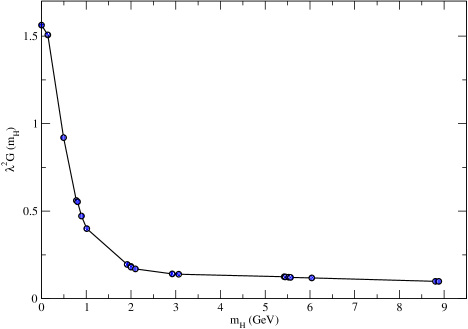
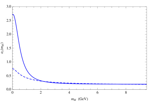
Figure 1: The dependence of the Fermi coupling on the fitted meson masses.

Figure 2: The comparison of the effective coupling $\alpha_{s}(m_{H})$ obtained in Ganbold:2010bu ; Ganbold:2012zz (dashed line) with our calculated dimensionless coupling $\lambda^{2}G(m_{H})$ (solid line) scaled to the curve $\alpha_{s}(m_{H})$ in the region of large masses.

V   Summary

We have represented a brief sketch of an approach to the bound state problem in quantum field theory which is based on the compositeness condition $Z_{H}=0$. By using the functional integral we have demonstrated explicitly that the four-fermion theory with the Fermi coupling $G$ is equivalent to the Yukawa-type theory if, first, the wave function renormalization constant in the Yukawa theory is equal to zero and, second, the Fermi coupling $G$ is inversely proportional to the meson mass function calculated for the physical meson mass.

We have given details for the calculation of the mass function for pseudoscalar and vector mesons in the framework of the covariant quark model. We updated the fit of the model parameters and calculated the Fermi coupling $G$ as a function of physical masses in a quite large region from the $\pi$ up to $B_{c}$ mesons.

We have suggested a smoothness criterion for the curve just varying the meson masses in such a way to obtain the smooth behavior for the Fermi coupling $G$. The mass spectrum obtained in this manner is found to be in good agreement with the experimental data. We have compared the behavior of $G$ with the strong QCD coupling $\alpha_{s}$ calculated in the QCD-inspired approach.

- (1) B. Jouvet, Nuovo Cim. 3, 1133 (1956).
- (2) A. Salam, Nuovo Cim. 25, 224 (1962).
- (3) M. A. Braun, Nucl. Phys. B 14, 413 (1969). (see, also Nucl. Phys. B 1, 277 (1967); B 5, 392 (1968) ).
- (4) S. Weinberg, Phys. Rev. 130, 776 (1963).
- (5) D. Lurie, Particles and fields, (Interscience Publishers, John Wiley Sons, New York, London, Sydney, 1968.)
- (6) K. Hayashi, M. Hirayama, T. Muta, N. Seto and T. Shirafuji, Fortsch. Phys. 15, 625 (1967).
- (7) I. V. Anikin, M. A. Ivanov, N. B. Kulimanova and V. E. Lyubovitskij, Z. Phys. C 65, 681 (1995).
- (8) Y. V. Burdanov, G. V. Efimov, S. N. Nedelko and S. A. Solunin, Phys. Rev. D 54, 4483 (1996).
- (9) G. V. Efimov and G. Ganbold, Phys. Rev. D 65, 054012 (2002); G. Ganbold, AIP Conf. Proc. 717, 285 (2004); ibid 796, 127 (2005).
- (10) G. Ganbold, Phys. Rev. D 79, 034034 (2009).
- (11) G. Ganbold, Phys. Rev. D 81, 094008 (2010).
- (12) G. Ganbold, Phys. Part. Nucl. 43, 79 (2012).
- (13) G. Ganbold, Phys. Part. Nucl. 45, 10 (2014).
- (14) G. V. Efimov and M. A. Ivanov, Int. J. Mod. Phys. A 4, 2031 (1989).
- (15) G. V. Efimov and M. A. Ivanov, The Quark Confinement Model of Hadrons, (IOP Publishing, Bristol Philadelphia, 1993).
- (16) M. A. Ivanov, J. G. Körner and P. Santorelli, Phys. Rev. D 71, 094006 (2005) [Erratum-ibid. D 75, 019901 (2007)]; Phys. Rev. D 73, 054024 (2006); Phys. Rev. D 70, 014005 (2004); Phys. Rev. D 63, 074010 (2001); A. Faessler, T. Gutsche, M. A. Ivanov, J. G. Körner and V. E. Lyubovitskij, Eur. Phys. J. direct C 4, 18 (2002); M. A. Ivanov and P. Santorelli, Phys. Lett. B 456, 248 (1999); M. A. Ivanov and V. E. Lyubovitskij, Phys. Lett. B 408, 435 (1997).
- (17) A. Faessler, T. Gutsche, M. A. Ivanov, J. G. Körner and V. E. Lyubovitskij, Phys. Rev. D 80, 034025 (2009); and V. E. Lyubovitskij, Phys. Lett. B 518, 55 (2001); A. Faessler, T. Gutsche, B. R. Holstein, M. A. Ivanov, J. G. Körner and V. E. Lyubovitskij, Phys. Rev. D 78, 094005 (2008); A. Faessler, T. .Gutsche, M. A. Ivanov, J. G. Körner, V. E. Lyubovitskij, D. Nicmorus and K. Pumsa-ard, Phys. Rev. D 73, 094013 (2006); M. A. Ivanov, J. G. Körner, V. E. Lyubovitskij and A. G. Rusetsky, Phys. Rev. D 60, 094002 (1999); M. A. Ivanov, V. E. Lyubovitskij, J. G. Körner and P. Kroll, Phys. Rev. D 56, 348 (1997); M. A. Ivanov, M. P. Locher and V. E. Lyubovitskij, Few Body Syst. 21, 131 (1996).
- (18) T. Branz, A. Faessler, T. Gutsche, M. A. Ivanov, J. G. Körner, V. E. Lyubovitskij, Phys. Rev. D81, 034010 (2010).
- (19) M. A. Ivanov, J. G. Körner, S. G. Kovalenko, P. Santorelli and G. G. Saidullaeva, Phys. Rev. D 85, 034004 (2012).
- (20) S. Dubnicka, A. Z. Dubnickova, M. A. Ivanov and A. Liptaj, Phys. Rev. D 87, 074201 (2013); T. Gutsche, M. A. Ivanov, J. G. Körner, V. E. Lyubovitskij and P. Santorelli, Phys. Rev. D 88, 114018 (2013); Phys. Rev. D 87, 074031 (2013); Phys. Rev. D 86, 074013 (2012).
- (21) S. Dubnicka, A. Z. Dubnickova, M. A. Ivanov and J. G. Körner, Phys. Rev. D 81, 114007 (2010); S. Dubnicka, A. Z. Dubnickova, M. A. Ivanov, J. G. Koerner, P. Santorelli and G. G. Saidullaeva, Phys. Rev. D 84, 014006 (2011).
- (22) S. Dubnicka, A. Z. Dubnickova, M. A. Ivanov and A. Liptaj, Phys. Rev. D 87, 074201 (2013).
- (23) J. Beringer et al. [Particle Data Group Collaboration], Phys. Rev. D 86, 010001 (2012).
- (24) J. L. Rosner, S. Stone, [arXiv:1002.1655 [hep-ex]].
- (25) J. Laiho, E. Lunghi, R. S. Van de Water, Phys. Rev. D81, 034503 (2010).
- (26) T. -W. Chiu et al. [ TWQCD Collaboration ], Phys. Lett. B651, 171-176 (2007).
- (27) D. Becirevic, P. Boucaud, J. P. Leroy, V. Lubicz, G. Martinelli, F. Mescia, F. Rapuano, Phys. Rev. D60, 074501 (1999).