Comments on the $U(1)$ axial symmetry and the chiral transition in QCD

Abstract

We analyze (using a chiral effective Lagrangian model) the scalar and pseudoscalar meson mass spectrum of QCD at finite temperature, above the chiral transition at $T_{c}$, looking, in particular, for signatures of a possible breaking of the $U(1)$ axial symmetry above $T_{c}$. A detailed comparison between the case with a number of light quark flavors $N_{f}\geq 3$ and the (remarkably different) case $N_{f}=2$ is performed.

1 Introduction

The so-called chiral condensate, $\langle\bar{q}q\rangle\equiv\sum_{l=1}^{N_{f}}\langle\bar{q}_{l}q_{l}\rangle$, is known to be an order parameter for the $SU(N_{f})\otimes SU(N_{f})$ chiral symmetry of the QCD Lagrangian with $N_{f}$ massless quarks (chiral limit), the physically relevant cases being $N_{f}=2$ and $N_{f}=3$. Lattice determinations of $\langle\bar{q}q\rangle$ (see, e.g., Refs. [1]) show that there is a chiral phase transition at a temperature $T_{c}\sim 150\div 170$ MeV, which is practically equal to the deconfinement temperature $T_{d}$, separating the confined (or hadronic) phase at $T<T_{d}$, from the deconfined phase (also known as quark-gluon plasma) at $T>T_{d}$. For $T<T_{c}\sim T_{d}$, the chiral condensate $\langle\bar{q}q\rangle$ is nonzero and the chiral symmetry is spontaneously broken down to the vectorial subgroup $SU(N_{f})_{V}$, and the $N_{f}^{2}-1$ $J^{P}=0^{-}$ lightest mesons are just the (pseudo-)Goldstone bosons associated with this breaking. Instead, for $T>T_{c}\sim T_{d}$, the chiral condensate $\langle\bar{q}q\rangle$ vanishes and the chiral symmetry is restored. But this is not the whole story, since QCD with $N_{f}$ massless quarks also has a $U(1)$ axial symmetry [$U(1)_{A}$], which is broken by an anomaly at the quantum level [2, 3]: this anomaly plays a fundamental role in explaining the large mass of the $\eta^{\prime}$ meson [4, 5].

Now, the question is: What is the role of the $U(1)$ axial symmetry for the finite temperature phase structure of QCD? One expects that, at least for $T\gg T_{c}$, where the density of instantons is strongly suppressed due to a Debye-type screening [6]), also the $U(1)$ axial symmetry will be (effectively) restored. This question is surely of phenomenological relevance since the particle mass spectrum above $T_{c}$ drastically depends on the presence or absence of the $U(1)$ axial symmetry. From the theoretical point of view, this question can be investigated by comparing (e.g., on the lattice) the behavior at nonzero temperatures of the two-point correlation functions $\langle O_{f}(x)O_{f}^{\dagger}(0)\rangle$ for the various $q\bar{q}$ meson channels (“$f$”). For example, for $N_{f}=2$ [7, 8], one can study the meson channels (traditionally called $\sigma$, $\vec{\delta}$, $\eta$ and $\vec{\pi}$) which are listed in Table 1, together with their corresponding interpolating operators and their isospin ($I$) and spin-parity ($J^{P}$) quantum numbers.

Meson channel	Interpolating operator	$I$	$J^{P}$
$\sigma$ (or $f_{0}$)	$O_{\sigma}=\overline{q}q$	0	$0^{+}$
$\vec{\delta}$ (or $\vec{a}_{0}$)	$\vec{O}_{\delta}=\overline{q}\frac{\vec{\tau}}{2}q$	1	$0^{+}$
$\eta$	$O_{\eta}=i\overline{q}\gamma_{5}q$	0	$0^{-}$
$\vec{\pi}$	$\vec{O}_{\pi}=i\overline{q}\gamma_{5}\frac{\vec{\tau}}{2}q$	1	$0^{-}$

Table 1: $q\bar{q}$ meson channels (for $N_{f}=2$) and their quantum numbers.

Under $SU(2)_{A}$ and $U(1)_{A}$ transformations, the $q\bar{q}$ meson channels are mixed as follows:

$$\begin{matrix}\sigma&\stackrel{{\scriptstyle U(1)_{A}}}{{\longleftrightarrow}}&\eta\\ SU(2)_{A}\updownarrow&&\updownarrow SU(2)_{A}\\ \vec{\pi}&\stackrel{{\scriptstyle U(1)_{A}}}{{\longleftrightarrow}}&\vec{\delta}\end{matrix}$$ (1)

The restoration of the $SU(2)$ chiral symmetry implies that the $\sigma$ and $\vec{\pi}$ channels become degenerate, with identical correlators and, therefore, with identical (screening) masses, $M_{\sigma}=M_{\pi}$. The same happens also for the channels $\eta$ and $\vec{\delta}$. Instead, an effective restoration of the $U(1)$ axial symmetry should imply that $\sigma$ becomes degenerate with $\eta$, and $\vec{\pi}$ becomes degenerate with $\vec{\delta}$. (Clearly, if both chiral symmetries are restored, then all $\sigma$, $\vec{\pi}$, $\eta$, and $\vec{\delta}$ correlators should become the same.)

In Ref. [9] the scalar and pseudoscalar meson mass spectrum, above the chiral transition at $T_{c}$, has been analyzed using, instead, a chiral effective Lagrangian model (which was originally proposed in Refs. [10, 11, 12] and elaborated on in Refs. [13, 14, 15]), which, in addition to the usual chiral condensate $\langle\bar{q}q\rangle$, also includes a (possible) genuine $U(1)_{A}$-breaking condensate that (possibly) survives across the chiral transition at $T_{c}$, staying different from zero at $T>T_{c}$. The motivations for considering this Lagrangian (and a critical comparison with other effective Lagrangian models existing in the literature) are recalled in Sec. 2. The results for the mesonic mass spectrum for $T>T_{c}$ are summarized in Sec. 3, for the case $N_{f}\geq 3$, and in Sec. 4, for the case $N_{f}=2$. Finally, in Sec. 5, we shall make some comments on (i) the remarkable difference between the case $N_{f}\geq 3$ and the case $N_{f}=2$, and (ii) the comparison between our results and the available lattice results for $N_{f}=2$ (or $N_{f}=2+1$).

2 Chiral effective Lagrangians

Chiral symmetry restoration at nonzero temperature is often studied in the framework of the following effective Lagrangian [16, 17, 18, 19, 20], written in terms of the (quark-bilinear) mesonic effective field $U_{ij}\sim\overline{q}_{jR}q_{iL}=\overline{q}_{j}\left(\frac{1+\gamma_{5}}{2}\right)q_{i}$,

$$\mathcal{L}_{1}(U,U^{\dagger})=\mathcal{L}_{0}(U,U^{\dagger})+\frac{B_{m}}{2\sqrt{2}}\mathrm{Tr}[MU+M^{\dagger}U^{\dagger}]$$ (2)

$$~{}~{}~{}~{}~{}~{}~{}~{}~{}~{}~{}~{}+\mathcal{L}_{I}(U,U^{\dagger}),$$

where $M={\rm diag}(m_{1},\dots,m_{N_{f}})$ is the quark mass matrix and $\mathcal{L}_{0}(U,U^{\dagger})$ is a term describing a kind of linear sigma model,

$$\begin{split}\mathcal{L}_{0}(U,U^{\dagger})=&~{}\frac{1}{2}\mathrm{Tr}[\partial_{\mu}U\partial^{\mu}U^{\dagger}]-V_{0}(U,U^{\dagger}),\\ V_{0}(U,U^{\dagger})=&~{}\frac{1}{4}\lambda_{\pi}^{2}\mathrm{Tr}[(UU^{\dagger}-\rho_{\pi}\mathbf{I})^{2}]+\frac{1}{4}\lambda_{\pi}^{\prime 2}[\mathrm{Tr}(UU^{\dagger})]^{2},\end{split}$$ (3)

while $\mathcal{L}_{I}(U,U^{\dagger})$ is an interaction term of the form:

$$\mathcal{L}_{I}(U,U^{\dagger})=c_{I}[\det U+\det U^{\dagger}].$$ (4)

Since under $U(N_{f})_{L}\otimes U(N_{f})_{R}$ chiral transformations the quark fields and the mesonic effective field $U$ transform as

$$U(N_{f})_{L}\otimes U(N_{f})_{R}:~{}q_{L,R}\rightarrow V_{L,R}q_{L,R}~{}\Rightarrow~{}U\rightarrow V_{L}UV_{R}^{\dagger},$$ (5)

where $V_{L}$ and $V_{R}$ are arbitrary $N_{f}\times N_{f}$ unitary matrices, we have that $\mathcal{L}_{0}(U,U^{\dagger})$ is invariant under the entire chiral group $U(N_{f})_{L}\otimes U(N_{f})_{R}$, while the interaction term (4) [and so the entire effective Lagrangian (2) in the chiral limit $M=0$] is invariant under $SU(N_{f})_{L}\otimes SU(N_{f})_{R}\otimes U(1)_{V}$ but not under a $U(1)$ axial transformation:

$$U(1)_{A}:~{}q_{L,R}\rightarrow e^{\mp i\alpha}q_{L,R}~{}\Rightarrow~{}U\rightarrow e^{-i2\alpha}U.$$ (6)

However, as was noticed by Witten [21], Di Vecchia, and Veneziano [22], this type of anomalous term does not correctly reproduce the U(1) axial anomaly of the fundamental theory, i.e., of the QCD (and, moreover, it is inconsistent with the $1/N_{c}$ expansion). In fact, one should require that, under a $U(1)$ axial transformation (6), the effective Lagrangian, in the chiral limit $M=0$, transforms as

$$U(1)_{A}:~{}\mathcal{L}^{(M=0)}_{eff}\rightarrow\mathcal{L}^{(M=0)}_{eff}+\alpha 2N_{f}Q,$$ (7)

where $Q(x)=\frac{g^{2}}{64\pi^{2}}\varepsilon^{\mu\nu\rho\sigma}F_{\mu\nu}^{a}(x)F_{\rho\sigma}^{a}(x)$ is the topological charge density and $\mathcal{L}_{eff}$ also contains $Q$ as an auxiliary field. The correct effective Lagrangian, satisfying the transformation property (7), was derived in Refs. [21, 22, 23, 24, 25] and is given by

$$\mathcal{L}_{2}(U,U^{\dagger},Q)=\mathcal{L}_{0}(U,U^{\dagger})+\frac{B_{m}}{2\sqrt{2}}\mathrm{Tr}[MU+M^{\dagger}U^{\dagger}]$$ (8)

$$~{}+\frac{i}{2}Q\mathrm{Tr}[\log U-\log U^{\dagger}]+\frac{1}{2A}Q^{2},$$

where $A=-i\int d^{4}x\langle TQ(x)Q(0)\rangle|_{YM}$ is the so-called topological susceptibility in the pure Yang–Mills (YM) theory. After integrating out the variable $Q$ in the effective Lagrangian (8), we are left with

$$\mathcal{L}_{2}(U,U^{\dagger})=\mathcal{L}_{0}(U,U^{\dagger})+\frac{B_{m}}{2\sqrt{2}}\mathrm{Tr}[MU+M^{\dagger}U^{\dagger}]$$ (9)

$$~{}+\frac{1}{8}A\left\{\mathrm{Tr}[\log U-\log U^{\dagger}]\right\}^{2},$$

to be compared with Eqs. (2)–(4).

For studying the phase structure of the theory at finite temperature $T$, all the parameters appearing in the effective Lagrangian must be considered as functions of $T$. In particular, the parameter $\rho_{\pi}$, appearing in the first term of the potential $V_{0}(U,U^{\dagger})$ in Eq. (3), is responsible for the behavior of the theory across the chiral phase transition at $T=T_{c}$. Let us consider, for a moment, only the linear sigma model $\mathcal{L}_{0}(U,U^{\dagger})$, i.e., let us neglect both the anomalous symmetry-breaking term and the mass term in Eq. (9). If $\rho_{\pi}(T<T_{c})>0$, then the value $\overline{U}$ for which the potential $V_{0}$ is minimum (that is, in a mean-field approach, the vacuum expectation value of the mesonic field $U$) is different from zero and can be chosen to be

$$\overline{U}|_{\rho_{\pi}>0}=v\mathbf{I},~{}~{}~{}~{}v\equiv\frac{F_{\pi}}{\sqrt{2}}=\sqrt{\frac{\rho_{\pi}\lambda_{\pi}^{2}}{\lambda_{\pi}^{2}+N_{f}\lambda_{\pi}^{\prime 2}}},$$ (10)

which is invariant under the vectorial $U(N_{f})_{V}$ subgroup; the chiral symmetry is thus spontaneously broken down to $U(N_{f})_{V}$. Instead, if $\rho_{\pi}(T>T_{c})<0$, we have that

$$\overline{U}|_{\rho_{\pi}<0}=0,$$ (11)

and the chiral symmetry is realized à la Wigner–Weyl. The critical temperature $T_{c}$ for the chiral phase transition is thus, in this case, simply the temperature at which the parameter $\rho_{\pi}$ vanishes: $\rho_{\pi}(T_{c})=0$.

However, the anomalous term in Eq. (9) makes sense only in the low-temperature phase ($T<T_{c}$), and it is singular for $T>T_{c}$, where the vacuum expectation value of the mesonic field $U$ vanishes. On the contrary, the interaction term (4) behaves well both in the low- and high-temperature phases.

The above-mentioned problems can be overcome by considering a modified effective Lagrangian (which was originally proposed in Refs. [10, 11, 12] and elaborated on in Refs. [13, 14, 15]), which, in a sense, is an “extension” of both $\mathcal{L}_{1}$ and $\mathcal{L}_{2}$, having (i) the correct transformation property (7) under the chiral group, and (ii) an interaction term containing the determinant of the mesonic field $U$, of the kind of that in Eq. (4), assuming that there is a $U(1)_{A}$-breaking condensate that (possibly) survives across the chiral transition at $T_{c}$, staying different from zero up to a temperature $T_{U(1)}>T_{c}$. (Of course, it is also possible that $T_{U(1)}\to\infty$, as a limit case. Another possible limit case, i.e., $T_{U(1)}=T_{c}$, will be discussed in the concluding comments in Sec. 5.) The new $U(1)$ chiral condensate has the form $C_{U(1)}=\langle{\cal O}_{U(1)}\rangle$, where, for a theory with $N_{f}$ light quark flavors, ${\cal O}_{U(1)}$ is a $2N_{f}$-quark local operator that has the chiral transformation properties of [3, 26, 27] ${\cal O}_{U(1)}\sim{\det}(\bar{q}_{sR}q_{tL})+{\det}(\bar{q}_{sL}q_{tR})$, where $s,t=1,\dots,N_{f}$ are flavor indices. The color indices (not explicitly indicated) are arranged in such a way that (i) ${\cal O}_{U(1)}$ is a color singlet, and (ii) $C_{U(1)}=\langle{\cal O}_{U(1)}\rangle$ is a genuine $2N_{f}$-quark condensate, i.e., it has no disconnected part proportional to some power of the quark-antiquark chiral condensate $\langle\bar{q}q\rangle$; the explicit form of the condensate for the cases $N_{f}=2$ and $N_{f}=3$ is discussed in detail in the Appendix A of Ref. [15] (see also Refs. [12, 28]).

The modified effective Lagrangian is written in terms of the topological charge density $Q$, the mesonic field $U_{ij}\sim\bar{q}_{jR}q_{iL}$, and the new field variable $X\sim{\det}(\bar{q}_{sR}q_{tL})$, associated with the $U(1)$ axial condensate [10, 11, 12],

$$\mathcal{L}(U,U^{\dagger},X,X^{\dagger},Q)=\frac{1}{2}\mathrm{Tr}[\partial_{\mu}U\partial^{\mu}U^{\dagger}]+\frac{1}{2}\partial_{\mu}X\partial^{\mu}X^{\dagger}$$ (12)

$$-\ V(U,U^{\dagger},X,X^{\dagger})+\frac{i}{2}\omega_{1}Q\mathrm{Tr}[\log U-\log U^{\dagger}]$$

$$+\ \frac{i}{2}(1-\omega_{1})Q[\log X-\log X^{\dagger}]+\frac{1}{2A}Q^{2},$$

where the potential term $V(U,U^{\dagger},X,X^{\dagger})$ has the form

$$V(U,U^{\dagger},X,X^{\dagger})$$ (13)

$$=\frac{1}{4}\lambda_{\pi}^{2}\mathrm{Tr}[(UU^{\dagger}-\rho_{\pi}{\bf I})^{2}]+\frac{1}{4}\lambda_{\pi}^{\prime 2}[\mathrm{Tr}(UU^{\dagger})]^{2}$$

$$+\ \frac{1}{4}\lambda_{X}^{2}[XX^{\dagger}-\rho_{X}]^{2}-\frac{B_{m}}{2\sqrt{2}}\mathrm{Tr}[MU+M^{\dagger}U^{\dagger}]$$

$$-\ \frac{c_{1}}{2\sqrt{2}}[X^{\dagger}\det U+X\det U^{\dagger}].$$

Since under chiral $U(N_{f})_{L}\otimes U(N_{f})_{R}$ transformations [see Eq. (5)] the field $X$ transforms exactly as $\det U$,

$$U(N_{f})_{L}\otimes U(N_{f})_{R}:~{}X\rightarrow\det V_{L}(\det V_{R})^{*}X,$$ (14)

[i.e., $X$ is invariant under $SU(N_{f})_{L}\otimes SU(N_{f})_{R}\otimes U(1)_{V}$, while, under a $U(1)$ axial transformation (6), $X\rightarrow e^{-i2N_{f}\alpha}X$], we have that, in the chiral limit $M=0$, the effective Lagrangian (12) is invariant under $SU(N_{f})_{L}\otimes SU(N_{f})_{R}\otimes U(1)_{V}$, while under a $U(1)$ axial transformation, it correctly transforms as in Eq. (7).

After integrating out the variable $Q$ in the effective Lagrangian (12), we are left with

$$\mathcal{L}(U,U^{\dagger},X,X^{\dagger})=\frac{1}{2}\mathrm{Tr}[\partial_{\mu}U\partial^{\mu}U^{\dagger}]+\frac{1}{2}\partial_{\mu}X\partial^{\mu}X^{\dagger}$$ (15)

$$~{}~{}~{}~{}~{}~{}~{}~{}~{}~{}~{}~{}~{}~{}~{}~{}~{}~{}~{}~{}-\tilde{V}(U,U^{\dagger},X,X^{\dagger}),$$

where

$$\tilde{V}=V-\frac{1}{8}A\{\omega_{1}\mathrm{Tr}[\log U-\log U^{\dagger}]$$ (16)

$$+\ (1-\omega_{1})[\log X-\log X^{\dagger}]\}^{2}.$$

As we have already said, all the parameters appearing in the effective Lagrangian must be considered as functions of the physical temperature $T$. In particular, the parameters $\rho_{\pi}$ and $\rho_{X}$ determine the expectation values $\langle U\rangle$ and $\langle X\rangle$, and so they are responsible for the behavior of the theory across the $SU(N_{f})\otimes SU(N_{f})$ and the $U(1)$ chiral phase transitions. We shall assume that the parameters $\rho_{\pi}$ and $\rho_{X}$, as functions of the temperature $T$, behave as reported in Table 2; $T_{\rho_{\pi}}$ is thus the temperature at which the parameter $\rho_{\pi}$ vanishes, while $T_{U(1)}>T_{\rho_{\pi}}$ is the temperature at which the parameter $\rho_{X}\,$ vanishes (with, as we have said above, $T_{U(1)}\to\infty$, i.e., $\rho_{X}\,>0$ $\forall T$, as a possible limit case).

$T<T_{\rho_{\pi}}$	$T_{\rho_{\pi}}<T<T_{U(1)}$	$T>T_{U(1)}$
$\rho_{\pi}>0$	$\rho_{\pi}<0$	$\rho_{\pi}<0$
$\rho_{X}\,>0$	$\rho_{X}\,>0$	$\rho_{X}\,<0$

Table 2: Dependence of the parameters $\rho_{\pi}$, $\rho_{X}\,$ on the temperature $T$.

We shall see in the next section that, in the case $N_{f}\geq 3$, one has $T_{c}=T_{\rho_{\pi}}$ (exactly as in the case of the linear sigma model $\mathcal{L}_{0}$ discussed above), while, as we shall see in Sec. 4, the situation in which $N_{f}=2$ is more complicated, being $T_{\rho_{\pi}}<T_{c}<T_{U(1)}$ in that case (unless $T_{\rho_{\pi}}=T_{c}=T_{U(1)}$; this limit case will be discussed in the concluding comments in Sec. 5).

Concerning the parameter $\omega_{1}$, in order to avoid a singular behavior of the anomalous term in Eq. (16) above the chiral transition temperature $T_{c}$, where the vacuum expectation value of the mesonic field $U$ vanishes (in the chiral limit $M=0$), we shall assume that $\omega_{1}(T\geq T_{c})=0$.

Finally, let us observe that the interaction term between the $U$ and $X$ fields in Eq. (13), i.e.,

$$\mathcal{L}_{int}=\frac{c_{1}}{2\sqrt{2}}[X^{\dagger}\det U+X\det U^{\dagger}],$$ (17)

is very similar to the interaction term (4) that we have discussed above for the effective Lagrangian $\mathcal{L}_{1}$. However, the term (17) is not anomalous, being invariant under the chiral group $U(N_{f})_{L}\otimes U(N_{f})_{R}$, by virtue of Eqs. (5) and (14). Nevertheless, if the field $X$ has a (real) nonzero vacuum expectation value $\overline{X}$ [the $U(1)$ axial condensate], then we can write

$$X=(\overline{X}+h_{X})e^{i\frac{S_{X}}{\overline{X}}}~{}~{}~{}~{}({\rm with:}~{}~{}\overline{h}_{X}=\overline{S}_{X}=0),$$ (18)

and, after susbstituting this in Eq. (17) and expanding in powers of the excitations $h_{X}$ and $S_{X}$, one recovers, at the leading order, an interaction term of the form (4):

$$\mathcal{L}_{int}=c_{I}[\det U+\det U^{\dagger}]+\dots,~{}~{}~{}~{}c_{I}\equiv\frac{c_{1}\overline{X}}{2\sqrt{2}}.$$ (19)

In what follows (see Ref. [9] for more details) we shall analyze the effects of assuming a nonzero value of the $U(1)$ axial condensate $\overline{X}$ on the scalar and pseudoscalar meson mass spectrum above the chiral transition temperature ($T>T_{c}$), both for the case $N_{f}\geq 3$ (Sec. 3) and for the case $N_{f}=2$ (Sec. 4).

3 Mass spectrum for $T>T_{c}$ in the case $N_{f}\geq 3$

Let us suppose to be in the range of temperatures $T_{\rho_{\pi}}<T<T_{U(1)}$, where, according to Table 2,

$$\rho_{\pi}\equiv-\frac{1}{2}B_{\pi}^{2}<0,~{}~{}~{}~{}\rho_{X}\,\equiv\frac{1}{2}F_{X}^{2}>0.$$ (20)

Since we expect that, due to the sign of the parameter $\rho_{X}$ in the potential (13), the $U(1)$ axial symmetry is broken by a nonzero vacuum expectation value of the field $X$ (at least for $\lambda_{X}^{2}\to\infty$ we should have $\overline{X}^{\dagger}\overline{X}\to\frac{1}{2}F_{X}^{2}$), we shall use for the field $U$ a simple linear parametrization, while, for the field $X$, we shall use a nonlinear parametrization (in the form of a polar decomposition),

$$U_{ij}=a_{ij}+ib_{ij},\,\,\,\,X=\alpha e^{i\beta}=(\overline{\alpha}+h_{X})e^{i\left(\overline{\beta}+\frac{S_{X}}{\overline{\alpha}}\right)},$$ (21)

where $\overline{X}=\overline{\alpha}e^{i\overline{\beta}}$ (with $\overline{\alpha}\neq 0$) is the vacuum expectation value of $X$ and $a_{ij}$, $b_{ij}$, $h_{X}$, and $S_{X}$ are real fields. Inserting Eq. (21) into the expressions (13) and (16), we find the expressions for the potential with and without the anomalous term (with $\omega_{1}=0$),

$$\tilde{V}=V-\frac{1}{8}A[\log X-\log X^{\dagger}]^{2}=V+\frac{1}{2}A\beta^{2},$$ (22)

$$\begin{split}V=&~{}\frac{1}{4}\lambda_{\pi}^{2}\mathrm{Tr}[(UU^{\dagger})(UU^{\dagger})]+\frac{1}{4}\lambda_{\pi}^{\prime 2}[\mathrm{Tr}(UU^{\dagger})]^{2}\\ &+\frac{1}{4}\lambda_{\pi}^{2}B_{\pi}^{2}(a_{ij}^{2}+b_{ij}^{2})+\frac{1}{4}\lambda_{X}^{2}\left(\alpha^{2}-\frac{1}{2}F_{X}^{2}\right)^{2}\\ &-\frac{B_{m}}{\sqrt{2}}m_{i}a_{ii}-\frac{c_{1}}{2\sqrt{2}}[\alpha\cos\beta(\det U+\det U^{\dagger})\\ &+i\alpha\sin\beta(\det U-\det U^{\dagger})]+\frac{N_{f}}{16}\lambda_{\pi}^{2}B_{\pi}^{4}.\end{split}$$

At the minimum of the potential we find that, at the leading order in $M={\rm diag}(m_{1},\dots,m_{N_{f}})$:

$$\overline{U}=\frac{2B_{m}}{\sqrt{2}\lambda_{\pi}^{2}B_{\pi}^{2}}M+\dots,~{}~{}\overline{\alpha}=\frac{F_{X}}{\sqrt{2}}+{\cal O}(\det M),~{}~{}\overline{\beta}=0.$$ (23)

In particular, in the chiral limit $M=0$, we find that $\overline{U}=0$ and $\overline{X}=\overline{\alpha}=\frac{F_{X}}{\sqrt{2}}$, which means that, in this range of temperatures $T_{\rho_{\pi}}<T<T_{U(1)}$, the $SU(N_{f})_{L}\otimes SU(N_{f})_{R}$ chiral symmetry is restored so that we can say that (at least for $N_{f}\geq 3$) $T_{c}\equiv T_{\rho_{\pi}}$, while the $U(1)$ axial symmetry is broken by the $U(1)$ axial condensate $\overline{X}$. Concerning the mass spectrum of the effective Lagrangian, we have $2N_{f}^{2}$ degenerate scalar and pseudoscalar mesonic excitations, described by the fields $a_{ij}$ and $b_{ij}$, plus a scalar ($0^{+}$) singlet field $h_{X}=\alpha-\overline{\alpha}$ and a pseudoscalar ($0^{-}$) singlet field $S_{X}=\overline{\alpha}\beta$ [see Eq. (21)], with squared masses given by

$$M^{2}_{U}=\frac{1}{2}\lambda_{\pi}^{2}B_{\pi}^{2},~{}~{}~{}M^{2}_{h_{X}}=\lambda_{X}^{2}F_{X}^{2},~{}~{}~{}M^{2}_{S_{X}}=\frac{A}{\overline{X}^{2}}=\frac{2A}{F_{X}^{2}}.$$ (24)

While the mesonic excitations described by the field $U$ are of the usual $q\bar{q}$ type, the scalar singlet field $h_{X}$ and the pseudoscalar singlet field $S_{X}$ describe instead two exotic, $2N_{f}$-quark excitations of the form $h_{X}~{}(\alpha)\sim{\det}(\bar{q}_{sL}q_{tR})+{\det}(\bar{q}_{sR}q_{tL})$ and $S_{X}\sim i[{\det}(\bar{q}_{sL}q_{tR})-{\det}(\bar{q}_{sR}q_{tL})]$. In particular, the physical interpretation of the pseudoscalar singlet excitation $S_{X}$ is rather obvious, and it was already discussed in Ref. [10]: it is nothing but the would-be Goldstone particle coming from the breaking of the $U(1)$ axial symmetry. In fact, neglecting the anomaly, it has zero mass in the chiral limit of zero quark masses. Yet, considering the anomaly, it acquires a topological squared mass proportional to the topological susceptibility $A$ of the pure YM theory, as required by the Witten–Veneziano mechanism [4, 5].

4 Mass spectrum for $T>T_{c}$ in the case $N_{f}=2$

As in the previous section, we start considering the range of temperatures $T_{\rho_{\pi}}<T<T_{U(1)}$, with the parameters $\rho_{\pi}$ and $\rho_{X}$ given by Eq. (20) (see also Table 2). We shall use for the field $U$ a more convenient variant of the linear parametrization, while, for the field $X$, we shall use the usual nonlinear parametrization given in Eq. (21),

$$U=\frac{1}{\sqrt{2}}[(\sigma+i\eta)\mathbf{I}+(\vec{\delta}+i\vec{\pi})\cdot\vec{\tau}],~{}~{}~{}~{}X=\alpha e^{i\beta},$$ (25)

where $\tau^{a}$ ($a=1,2,3$) are the three Pauli matrices [with the usual normalization $\mathrm{Tr}(\tau^{a}\tau^{b})=2\delta_{ab}$] and the fields $\sigma$, $\eta$, $\vec{\delta}$, and $\vec{\pi}$ describe, precisely, the $q\bar{q}$ mesonic excitations which are listed in Table 1.

Inserting Eq. (25) and $M={\rm diag}(m_{u},m_{d})$ into the expressions (13) and (16), we find the following expression for the potential with and without the anomalous term (with $\omega_{1}=0$),

$$\tilde{V}=V-\frac{1}{8}A[\log X-\log X^{\dagger}]^{2}=V+\frac{1}{2}A\beta^{2},~{}~{}~{}~{}~{}~{}~{}~{}~{}~{}$$ (26)

$$\begin{split}V=&~{}\frac{1}{4}\lambda_{\pi}^{2}\mathrm{Tr}[(UU^{\dagger})(UU^{\dagger})]+\frac{1}{4}\lambda_{\pi}^{\prime 2}[\mathrm{Tr}(UU^{\dagger})]^{2}\\ &+\frac{1}{4}\lambda_{\pi}^{2}B_{\pi}^{2}[\sigma^{2}+\eta^{2}+\vec{\delta}^{2}+\vec{\pi}^{2}]+\frac{1}{4}\lambda_{X}^{2}\left(\alpha^{2}-\frac{1}{2}F_{X}^{2}\right)^{2}\\ &-\frac{B_{m}}{2}[(m_{u}+m_{d})\sigma+(m_{u}-m_{d})\delta_{3}]\\ &-\frac{c_{1}}{2\sqrt{2}}[\alpha\cos\beta(\sigma^{2}-\eta^{2}-\vec{\delta}^{2}+\vec{\pi}^{2})\\ &+2\alpha\sin\beta(\sigma\eta-\vec{\delta}\cdot\vec{\pi})]+\frac{1}{8}\lambda_{\pi}^{2}B_{\pi}^{4}.\end{split}$$

When studying the equations for a stationary point of the potential, one immediately finds that $\overline{\eta}=\overline{\pi}_{a}=\overline{\beta}=0$ ($P$-invariance requires that $\overline{U}=\overline{U}^{\dagger}$ and $\overline{X}=\overline{X}^{\dagger}$), and also $\overline{\delta}_{1}=\overline{\delta}_{2}=0$, while for the other values $\overline{\alpha}$, $\overline{\sigma}$ and $\overline{\delta}\equiv\overline{\delta}_{3}$ one finds the following solution (at the first nontrivial order in the quark masses):

$$\overline{\sigma} = \frac{B_{m}}{\lambda_{\pi}^{2}B_{\pi}^{2}-c_{1}F_{X}}(m_{u}+m_{d})+\dots,$$

$$\overline{\delta} = \frac{B_{m}}{\lambda_{\pi}^{2}B_{\pi}^{2}+c_{1}F_{X}}(m_{u}-m_{d})+\dots,$$

$$\overline{\alpha} = \frac{F_{X}}{\sqrt{2}}+{\cal O}(m^{2}),$$ (27)

which, in the chiral limit $m_{u}=m_{d}=0$, reduces to

$$\overline{U}=0,~{}~{}~{}~{}\overline{X}=\overline{\alpha}=\frac{F_{X}}{\sqrt{2}},$$ (28)

signalling that the $SU(2)_{L}\otimes SU(2)_{R}$ chiral symmetry is restored, while the $U(1)$ axial symmetry is broken by the $U(1)$ axial condensate $\overline{X}$.

Studying the matrix of the second derivatives (Hessian) of the potential with respect to the fields at the stationary point, one finds that (in the chiral limit $m_{u}=m_{d}=0$) there are (as in the case $N_{f}\geq 3$) two exotic $0^{\pm}$ singlet mesonic excitations, described by the fields $h_{X}=\alpha-\overline{\alpha}$ and $S_{X}=\overline{\alpha}\beta$, with squared masses $M^{2}_{h_{X}}=\lambda_{X}^{2}F_{X}^{2}$, $M^{2}_{S_{X}}=\frac{A}{\overline{X}^{2}}=\frac{2A}{F_{X}^{2}}$, and, moreover, two $q\bar{q}$ chiral multiplets appear in the mass spectrum of the effective Lagrangian, namely,

$$(\sigma,\vec{\pi}): ~{}M_{\sigma}^{2}=M_{\pi}^{2}=\frac{1}{2}(\lambda_{\pi}^{2}B_{\pi}^{2}-\sqrt{2}c_{1}\overline{X}),$$

$$(\eta,\vec{\delta}): ~{}M_{\eta}^{2}=M_{\delta}^{2}=\frac{1}{2}(\lambda_{\pi}^{2}B_{\pi}^{2}+\sqrt{2}c_{1}\overline{X}),$$ (29)

signalling the restoration of the $SU(2)_{L}\otimes SU(2)_{R}$ chiral symmetry. Instead, the squared masses of the $q\bar{q}$ mesonic excitations belonging to a same $U(1)$ chiral multiplet, such as $(\sigma,\eta)$ and $(\vec{\pi},\vec{\delta})$, remain split by the quantity

$$\Delta M_{U(1)}^{2}\equiv M_{\eta}^{2}-M_{\sigma}^{2}=M_{\delta}^{2}-M_{\pi}^{2}=\sqrt{2}c_{1}\overline{X},$$ (30)

proportional to the $U(1)$ axial condensate $\overline{X}=\frac{F_{X}}{\sqrt{2}}$. This result is to be contrasted with the corresponding result obtained in the previous section for the $N_{f}\geq 3$ case, see Eq. (24), in which all (scalar and pseudoscalar) $q\bar{q}$ mesonic excitations (described by the field $U$) turned out to be degenerate, with squared masses $M_{U}^{2}=\frac{1}{2}\lambda_{\pi}^{2}B_{\pi}^{2}$.

5 Comments on the results and conclusions

The difference in the mass spectrum of the $q\bar{q}$ mesonic excitations (described by the field $U$) for $T>T_{c}$ between the case $N_{f}=2$ and the case $N_{f}\geq 3$ is due to the different role of the interaction term $\mathcal{L}_{int}=c_{I}[\det U+\det U^{\dagger}]+\dots$, with $c_{I}\equiv\frac{c_{1}\overline{X}}{2\sqrt{2}}$, in the two cases. When $N_{f}=2$, this term is (at the lowest order) quadratic in the fields $U$ so that it contributes to the squared mass matrix. Instead, when $N_{f}\geq 3$, this term is (at the lowest order) an interaction term of order $N_{f}$ in the fields $U$ (e.g., a cubic interaction term for $N_{f}=3$) so that, in the chiral limit, when $\overline{U}=0$, it does not affect the masses of the $q\bar{q}$ mesonic excitations.

Alternatively, we can also explain the difference by using a “diagrammatic” approach, i.e., by considering, for example, the diagrams that contribute to the following quantity $\mathcal{D}_{U(1)}$, defined as the difference between the correlators for the $\delta^{+}$ and $\pi^{+}$ channels:

$$\begin{split}{\cal D}&{}_{U(1)}(x)\equiv\langle TO_{\delta^{+}}(x)O_{\delta^{+}}^{\dagger}(0)\rangle-\langle TO_{\pi^{+}}(x)O_{\pi^{+}}^{\dagger}(0)\rangle\\ &=2\left[\langle T\bar{u}_{R}d_{L}(x)\ \bar{d}_{R}u_{L}(0)\rangle+\langle T\bar{u}_{L}d_{R}(x)\ \bar{d}_{L}u_{R}(0)\rangle\right].\end{split}$$ (31)

What happens below and above $T_{c}$? For $T<T_{c}$, in the chiral limit $m_{1}=\dots~{}m_{N_{f}}=0$, the left-handed and right-handed components of a given light quark flavor can be connected through the $q\bar{q}$ chiral condensate, giving rise to a nonzero contribution to the quantity ${\cal D}_{U(1)}(x)$ in Eq. (31). But for $T>T_{c}$, the $q\bar{q}$ chiral condensate is zero, and, therefore, also the quantity ${\cal D}_{U(1)}(x)$ should be zero for $T>T_{c}$, unless there is a nonzero $U(1)$ axial condensate $\overline{X}$; in that case, one should also consider the diagram with the insertion of a $2N_{f}$-quark effective vertex associated with the $U(1)$ axial condensate $\overline{X}$. For $N_{f}=2$ (see Figure 1), all the left-handed and right-handed components of the up and down quark fields in Eq. (31) can be connected through the four-quark effective vertex, giving rise to a nonzero contribution to the quantity ${\cal D}_{U(1)}(x)$.

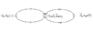
Figure 1: Diagram with the contribution to ${\cal D}_{U(1)}$ from the $2N_{f}$-quark effective vertex in the case $N_{f}=2$.

Instead, for $N_{f}=3$ (see Figure 2), the six-quark effective vertex also generates a couple of right-handed and left-handed strange quarks, which, for $T>T_{c}$, can only be connected through the mass operator $-m_{s}\overline{q}_{s}q_{s}$, so that (differently from the case $N_{f}=2$) this contribution to the quantity ${\cal D}_{U(1)}(x)$ should vanish in the chiral limit; this implies that, for $N_{f}=3$ and $T>T_{c}$, the $\vec{\delta}$ and $\vec{\pi}$ correlators are identical, and, as a consequence, also $M_{\delta}=M_{\pi}$.

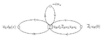
Figure 2: Diagram with the contribution to ${\cal D}_{U(1)}$ from the $2N_{f}$-quark effective vertex in the case $N_{f}=3$.

This argument can be easily generalized to include also the other meson channels and to the case $N_{f}>3$.

Finally, let us see how our results for the mass spectrum compare with the available lattice results. Lattice results for the case $N_{f}=2$ (and for the case $N_{f}=2+1$, with $m_{u,d}\to 0$ and $m_{s}\sim 100$ MeV) exist in the literature, even if the situation is, at the moment, a bit controversial. In fact, almost all lattice results [29, 30, 31, 32, 33, 34, 35, 36] (using staggered fermions or domain-wall fermions on the lattice) indicate the nonrestoration of the $U(1)$ axial symmetry above the chiral transition at $T_{c}$, in the form of a small (but nonzero) splitting between the $\vec{\delta}$ and $\vec{\pi}$ correlators above $T_{c}$, up to $\sim 1.2~{}T_{c}$. In terms of our result (30), we would interpret this by saying that, for $T>T_{c}$, there is still a nonzero $U(1)$ axial condensate, $\overline{X}>0$, so that $c_{I}=\frac{c_{1}\overline{X}}{2\sqrt{2}}>0$ and the above-mentioned interaction term, containing the determinant of the mesonic field $U$, is still effective for $T>T_{c}$.

However, other lattice results obtained in Ref. [37] (using the so-called overlap fermions on the lattice; see also Ref. [38]) do not show evidence of the above-mentioned splitting above $T_{c}$, so indicating an effective restoration of the $U(1)$ axial symmetry above $T_{c}$, at least, at the level of the $q\bar{q}$ mesonic mass spectrum. In terms of our result (30), we would interpret this by saying that, for $T>T_{c}$, one has $c_{1}\overline{X}=0$, so that $c_{I}=\frac{c_{1}\overline{X}}{2\sqrt{2}}=0$ and the above-mentioned interaction term, containing the determinant of the mesonic field $U$, is not present for $T>T_{c}$. For example, it could be that also the $U(1)$ axial condensate $\overline{X}$ (like the usual chiral condensate $\langle\bar{q}q\rangle$) vanishes at $T=T_{c}$, i.e., using the notation introduced in Sec. 2 (see Table 2), that $T_{U(1)}=T_{c}$. (Or, even more drastically, it could be that there is simply no genuine $U(1)$ axial condensate …)

In conclusion, further work will be necessary, both from the analytical point of view but especially from the numerical point of view (i.e., by lattice calculations), in order to unveil the persistent mystery of the fate of the $U(1)$ axial symmetry at finite temperature.

Also the question of the (possible) exotic pseudoscalar singlet field $S_{X}\sim i[{\det}(\bar{q}_{sL}q_{tR})-{\det}(\bar{q}_{sR}q_{tL})]$ for $T>T_{c}$, with squared mass (in the chiral limit) given by $M^{2}_{S_{X}}|_{M=0}=\frac{A}{\overline{X}^{2}}=\frac{2A}{F_{X}^{2}}$, should be further investigated, both theoretically and experimentally. As we have already said, the excitation $S_{X}$ is nothing but the would-be Goldstone particle coming from the breaking of the $U(1)$ axial symmetry, as required by the Witten–Veneziano mechanism [4, 5]. So, it is precisely what we should call the “$\eta^{\prime}$” for $T>T_{c}$: is there any chance to observe it? Lattice results seem to indicate that $A(T)$ has a sharp decrease for $T>T_{c}$ and it vanishes at $\sim 1.2~{}T_{c}$ [39]. (And, maybe, $A(T>T_{c})\to 0$ for $N_{c}\to\infty$, as it was suggested in Ref. [40].) Could this explain the “$\eta^{\prime}$” mass decrease, which, according to Ref. [41], has been observed inside the fireball in heavy-ion collisions?

References

-
[1]
F. Karsch, Lect. Notes Phys. 583 (2002) 209;
A. Bazavov et al. (HotQCD Collaboration), Phys. Rev. D 85 054503 (2012) 054503. - [2] S. Weinberg, Phys. Rev. D 11 (1975) 3583.
-
[3]
G. ’t Hooft, Phys. Rev. Lett. 37 (1976) 8;
G. ’t Hooft, Phys. Rev. D 14 (1976) 3432 [Erratum–ibid. 18 (1978) 2199]. - [4] E. Witten, Nucl. Phys. B 156 (1979) 269.
- [5] G. Veneziano, Nucl. Phys. B 159 (1979) 213.
- [6] D.J. Gross, R.D. Pisarski, and L.G. Yaffe, Rev. Mod. Phys. 53 (1981) 43.
-
[7]
C. DeTar and J. Kogut, Phys. Rev. Lett. 59 (1987) 399;
C. DeTar and J. Kogut, Phys. Rev. D 36 (1987) 2828. - [8] E. Shuryak, Comments Nucl. Part. Phys. 21 (1994) 235.
- [9] E. Meggiolaro and A. Mordà, Phys. Rev. D 88 (2013) 096010.
- [10] E. Meggiolaro, Z. Phys. C 62 (1994) 669.
- [11] E. Meggiolaro, Z. Phys. C 62 (1994) 679.
- [12] E. Meggiolaro, Z. Phys. C 64 (1994) 323.
- [13] M. Marchi and E. Meggiolaro, Nucl. Phys. B 665 (2003) 425.
- [14] E. Meggiolaro, Phys. Rev. D 69 (2004) 074017.
- [15] E. Meggiolaro, Phys. Rev. D 83 (2011) 074007.
- [16] R.D. Pisarski and F. Wilczek, Phys. Rev. D 29 (1984) 338.
- [17] G. ’t Hooft, Phys. Rep. 142 (1986) 357.
- [18] J.T. Lenaghan, D.H. Rischke, and J. Schaffner-Bielich, Phys. Rev. D 62 (2000) 085008.
- [19] D. Röder, J. Ruppert, and D. Rischke, Phys Rev. D 68 (2003) 016003.
-
[20]
A. Butti, A. Pelissetto, and E. Vicari, J. High Energy Phys. 08 (2003)
029;
F. Basile, A. Pelissetto, and E. Vicari, Proc. Sci. LAT2005 (2005) 199;
A. Pelissetto and E. Vicari, Phys. Rev. D 88 (2013) 105018. - [21] E. Witten, Ann. Phys. (N.Y.) 128 (1980) 363.
- [22] P. Di Vecchia and G. Veneziano, Nucl. Phys. B 171 (1980) 253.
- [23] C. Rosenzweig, J. Schechter, and C.G. Trahern, Phys. Rev. D 21 (1980) 3388.
- [24] K. Kawarabayashi and N. Ohta, Nucl. Phys. B 175 (1980) 477.
- [25] P. Nath and R. Arnowitt, Phys. Rev. D 23 (1981) 473.
- [26] M. Kobayashi and T. Maskawa, Prog. Theor. Phys. 44 (1970) 1422.
- [27] T. Kunihiro, Prog. Theor. Phys. 122 (2009) 255.
- [28] A. Di Giacomo and E. Meggiolaro, Nucl. Phys. B, Proc. Suppl. 42 (1995) 478.
-
[29]
C. Bernard et al., Nucl. Phys. B, Proc. Suppl. 53 (1997) 442;
C. Bernard, T. Blum, C. DeTar, S. Gottlieb, U. Heller, J. Hetrick, K. Rummukainen, R. Sugar, D. Toussaint, and M. Wingate, Phys. Rev. Lett. 78 (1997) 598. - [30] J.B. Kogut, J.-F. Lagaë, and D.K. Sinclair, Phys. Rev. D 58 (1998) 054504.
- [31] S. Chandrasekharan, D. Chen, N.H. Christ, W.-J. Lee, R. Mawhinney, and P.M. Vranas, Phys. Rev. Lett. 82 (1999) 2463.
- [32] F. Karsch, Nucl. Phys. B, Proc. Suppl. 83–84 (2000) 14.
- [33] P.M. Vranas, Nucl. Phys. B, Proc. Suppl. 83–84 (2000) 414.
- [34] M. Cheng et al., Eur. Phys. J. C 71 (2011) 1564.
- [35] A. Bazavov et al. (HotQCD Collaboration), Phys. Rev. D 86 (2012) 094503.
- [36] M.I. Buchoff et al. (LLNL/RBC Collaboration), Phys. Rev. D 89 (2014) 054514.
- [37] G. Cossu, S. Aoki, H. Fukaya, S. Hashimoto, T. Kaneko, H. Matsufuru, and J.-I. Noaki, Phys. Rev. D 87 (2013) 114514.
- [38] S. Aoki, H. Fukaya, and Y. Taniguchi, Phys. Rev. D 86 (2012) 114512.
- [39] E. Vicari and H. Panagopoulos, Phys. Rep. 470 (2009) 93.
- [40] D. Kharzeev, R.D. Pisarski, and M.H.G. Tytgat, Phys. Rev. Lett. 81 (1998) 512.
- [41] T. Csörgo, R. Vértesi, and J. Sziklai, Phys. Rev. Lett. 105 (2010) 182301.