A new configurational bias scheme for sampling supramolecular structures

Abstract

We present a new simulation scheme which allows an efficient sampling of reconfigurable supramolecular structures made of polymeric constructs functionalized by reactive binding sites. The algorithm is based on the configurational bias scheme of Siepmann and Frenkel and is powered by the possibility of changing the topology of the supramolecular network by a non–local Monte Carlo algorithm. Such plan is accomplished by a multi–scale modelling that merges coarse-grained simulations, describing the typical polymer conformations, with experimental results accounting for free energy terms involved in the reactions of the active sites. We test the new algorithm for a system of DNA coated colloids for which we compute the hybridisation free energy cost associated to the binding of tethered single stranded DNAs terminated by short sequences of complementary nucleotides. In order to demonstrate the versatility of our method, we also consider polymers functionalized by receptors that bind a surface decorated by ligands. In particular we compute the density of states of adsorbed polymers as a function of the number of ligand–receptor complexes formed. Such a quantity can be used to study the conformational properties of adsorbed polymers useful when engineering adsorption with tailored properties. We successfully compare the results with the predictions of a mean field theory. We believe that the proposed method will be a useful tool to investigate supramolecular structures resulting from direct interactions between functionalized polymers for which efficient numerical methodologies of investigation are still lacking.

I Introduction

Polymeric constructs functionalized by active groups that can selectively react with complementary groups are at the core of many biological systems (e.g. cell signaling and protein docking) and are becoming a very popular tool to engineer new functional materials in the field of nanotechnology.Mirkin et al. (1996); Alivisatos et al. (1996); Di Michele and Eiser (2013); Dubacheva et al. (2014); Kiessling and Grim (2013) For instance, DNA strands tipped by reactive sequences of single stranded (ss)DNA are currently used to mediate direct interactions between colloids,Mirkin et al. (1996); Alivisatos et al. (1996); Di Michele and Eiser (2013) in DNA origami to assist the assembly of DNA tiles into complex patterns,Han et al. (2011) or to design supramolecular gels.Biffi et al. (2013); Schmid (2013) Functionalized polymers are also used in nanomedicine, in particular in drug delivery to engineer selective targeting.Dubacheva et al. (2014); Martinez-Veracoechea and Frenkel (2011); Kiessling and Grim (2013)

Functionalized polymers are difficult to model because their properties result from a synergistic effect between the reaction free energy of the functional groups and the polymer conformations that are sharply constrained by the tight binding acting between reacting spots.Dreyfus et al. (2010); Leunissen and Frenkel (2011); Mognetti, Leunissen, and Frenkel (2012) These two contributions to the free energy are comparable (though usually of opposite sign) and, in the interesting regimes, are accessible by thermal fluctuations.Leunissen and Frenkel (2011) Hence a statistical mechanics treatment of these systems needs to account for these two effects.Mognetti et al. (2012); Varilly et al. (2012); Angioletti-Uberti et al. (2013)

This leads to a multi–scale problem that hampers the modelling of these systems. In particular an adequate description of the reactive binding sites requires atomistic models that become unpractical when sampling polymer conformations. This can be better explained by considering the two systems that will be treated in this paper. First we will study the hybridisation of tethered inert strands of ssDNA terminated by a reactive sequence as used in DNA coated colloids (DNACCs). Here a detailed model necessary to properly describe the hybridisation free energy of the reactive sequencesOuldridge, Louis, and Doye (2011) cannot be employed, in realistic computational time, to study typical DNACCs made of thousand of different ssDNA (long of up to 50 base pairs) terminated by short strings of active bases.Rogers and Crocker (2011) In a second system we will study the conformation and the density of states of functionalized polymers adsorbed by ligands distributed on a surface as motivated by recent experiments.Dubacheva et al. (2014) Similarly to the case of DNACCs, a proper sampling requires exploring many configurations grouped in different topologies in which different receptors bind different ligands. Realistic dynamics of atomistic models cannot access the timescales of such systems.

In this paper we study the possibility of designing non–local Monte Carlo (MC) moves to sample between supramolecular polymer configurations with different topologies. Specifically we propose an algorithm that could, in one step, bind/unbind two tethered strands in a system featuring DNA-mediated interactions or that could attach/detach a receptor of a functionalized polymer to/from a ligand tethered to a surface. In doing so we will employ a multi–scale approach in which the free energy of the reacting sites is taken into account implicitly, using accessible experimental results.

Some steps in this direction have already been taken.Mognetti et al. (2012); Varilly et al. (2012) In particular in Ref. Mognetti et al., 2012 we used MC Rosenbluth Sampling Frenkel and Smit (2001) to estimate the hybridisation free energy of tethered single stranded DNA constructs. Because Rosenbluth weights can be linked to the free energy of the constructs, Frenkel and Smit (2001) it is possible to calculate the configurational part of the hybridisation free energy by comparing independent Rosenbluth simulations of free and hybridised strands.

In this paper we want to extend these methods to a dynamic algorithm in which the supramolecular network is reconfigured on the fly. There are different reasons for aiming at this step. Notoriously the quality of the sampling in static Rosenbluth simulations becomes poor for long polymeric constructs.Mooij and Frenkel (1994); Batoulis and Kremer (1988) Moreover, from a more practical point of view, a dynamic scheme is much more versatile because it allows to study a broader range of systems for which pre–computing Rosenbluth weights (as done in Refs. Mognetti et al., 2012; Varilly et al., 2012) would be unfeasible. In particular this has motivated the study of the targeting problem presented in the second part of the paper.

This paper is organised as follows. In Sec. II we present our algorithm. We present the multi–scale approach, detail the algorithm by which supramolecular structures are generated, and derive the acceptance rules used to swap between them. In view of the similarity with the configurational bias MC (CBMC) scheme,Siepmann and Frenkel (1992) and of its ability to swap between configurations with different topologies, we label the new algorithm topological CBMC (tCBMC). In Sec. III we test tCBMC for DNA–coated colloids systems. In particular we show how tCBMC can measure the hybridisation free energy of two tethered constructs in agreement with previous studies.Mognetti et al. (2012); Varilly et al. (2012) In Sec. IV we then consider a polymer functionalized by receptors targeting ligands distributed on a surface. In particular we show how tCBMC, in tandem with a powerful umbrella sampling scheme,Virnau and Müller (2004) allows to compute the density of states of an adsorbed polymer as a function of the number of functionalized ligands. We validate our finding using a mean field (MF) theory that we present in appendix A. Finally in Sec. V we present the conclusions and the perspectives of our work.

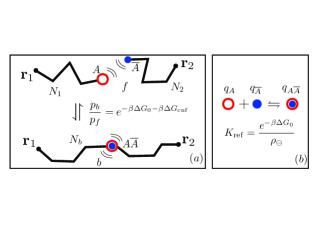
Figure 1: $(a)$ The hybridisation of two tethers functionalized by reactive sites is controlled by the hybridisation free energy of the free active groups in solutions $\Delta G_{0}$ $(b)$, and by a configurational term $\Delta G_{\mathrm{cnf}}$ due to the tethering constraint.

II The method

Fig. 1$a$ depicts the typical situation that we are interested in modelling. Two polymeric constructs, tethered in ${\bf r}_{1}$ and ${\bf r}_{2}$, are tipped by complementary reactive elements ($A$ and $\overline{A}$). We discern between two possible states in which the constructs are either free ($f$) or react giving rise to a bound state ($b$). In the latter case we say that a supramolecular structure, spanning between ${\bf r}_{1}$ and ${\bf r}_{2}$, has been formed. Here we introduce an algorithm that samples directly between configurations of type $f$ and of type $b$. For simplicity we keep the tethering points ${\bf r}_{1}$ and ${\bf r}_{2}$ fixed (this constraint can be removed combining the current technique with standard local algorithms).

Our coarse-grained approach does not model the atomistic details of the reactive elements. Instead we use implicit terms ($q_{A}$, $q_{\overline{A}}$ and $q_{A\overline{A}}$) as internal partition function of the active groups and bound complex ($A$, $\overline{A}$ and $A\overline{A}$, respectively). The internal partition functions can be linked to the equilibrium constant of the dimerisation reaction between free reacting groups in solution (Fig. 1$b$). In particular the equilibrium condition between the chemical potential of the reactants $\mu_{b}=\mu_{f1}+\mu_{f2}$ implies the following relationLeunissen and Frenkel (2011); Mognetti, Leunissen, and Frenkel (2012)

$${q_{A\overline{A}}\over q_{A}q_{\overline{A}}}=K_{\mathrm{ref}}={e^{-\beta\Delta G_{0}}\over\rho_{\ominus}}\,,$$ (1)

where $\rho_{\ominus}$ is the standard concentration. The partition functions of the free ($f$) and bound ($b$) tethers can then be derived summing over all the possible constructs’ configurations

$$Z_{f} = q_{A}q_{\overline{A}}\int{\mathrm{d}}c_{f}\,e^{-\beta H^{(f)}(c_{f})}\,,$$ (2)

$$Z_{b} = q_{A\overline{A}}\int{\mathrm{d}}c_{b}\,e^{-\beta H^{(b)}(c_{b})}\delta(f_{\mathrm{ee}}(c_{b})-r_{12})\,,$$ (3)

where $c_{f}$ represents two polymers emanating from ${\bf r}_{1}$ and ${\bf r}_{2}$, while $c_{b}$ is a single polymer branch (see Fig. 1). In Eq. 3 $f_{\mathrm{ee}}(c_{b})$ is the function that provides the end-to-end distance of a bound configuration ($c_{b}$) and we have defined $r_{12}=|{\bf r}_{1}-{\bf r}_{2}|$. In Eqs. 2 and 3 $H^{(f)}$ and $H^{(b)}$ are the configurational energies of the free and of the bound constructs. They also account for the interactions of the chain with the environment (hard walls, other polymers, etc.). In this study the polymeric constructs are modelled by flexible freely-jointed chains (FJCs) made of $N_{1}$ and $N_{2}$ segments for the free constructs and $N_{b}=N_{1}+N_{2}$ segments for the bound construct. The nature of $H^{(b)}$ and $H^{(f)}$ will be further specified in the next sections. The method of Fig. 1$a$ may resemble identity swap MC schemes that have been used, for instance, to sample populations of polymers with different lengths by removing monomers from longer chains and regrowing them at the end terminals of the shorter chains.Siepmann and McDonald (1992) However in Fig. 1$a$ we have to account for the loss of three degrees of freedom of the hybridised chain due to the fixed–end–point constraints.

Notice that we have used a point–like representation for the reactive elements. This may look limiting, for instance, in the case of DNACC systems where the length of the hybridised segments can be comparable with the Kuhn length of the constructs. In this regard, we observe that it is rather straightforward to generalise our procedure to more detailed models that include a non trivial representation of the reactive groups.

Here we explain how we create new polymer configurations. Like in Rosenbluth sampling, in order to generate free configurations $f$, we grow two open chains by sequentially adding $N_{1}$ and $N_{2}$ segments ${\bf u}_{i}$ starting from ${\bf r}_{1}$ and ${\bf r}_{2}$ respectively.Note (2) The $i$–$th$ segment (${\bf u}_{i}$) is sampled within $k$ possible ones (${\bf u}_{i,\alpha}$, with $\alpha=1,\cdots k$) that are generated with a uniform distribution. In this work we use $k=20$. The segment ${\bf u}_{i}$ is chosen within the $k$ possibilities with probability $p_{i,\alpha}\sim{\exp[-\beta H^{(f)}_{i}({\bf u}_{i,\alpha})]}$. $H^{(f)}_{i}({\bf u})$ is the interaction of the segment ${\bf u}$ with the surrounding environment, including the fraction of chains already grown.Frenkel and Smit (2001) If $W^{(f)}_{i}=k^{-1}\sum_{\alpha=1}^{k}\exp[-\beta H^{(f)}_{i}({\bf u}_{i,\alpha})]$, we can define the Rosenbluth weight of the newly generated configuration ($c_{f}$) in the standard way $W^{(f)}(c_{f})=\prod_{i=1}^{N_{b}}W^{(f)}_{i}$. Following the previous procedure, a free configuration $c_{f}$ is generated with probability

$$p(c_{f}) = {e^{-\beta H^{(f)}(c_{f})}\over W^{(f)}(c_{f})}\,.$$ (4)

A similar algorithm can be used to grow bound constructs $b$. However in this case we have to further bias the sampling to satisfy the distance constraint on the end points. If the $i-1$–$th$ segment terminates in ${\bf x}_{i-1}$, the $k$ possible segments are generated with probability distribution function given by the normalised density of FJCs made of $N_{b}-i$ segments with end point distance equal to $|{\bf r}_{2}-{\bf x}_{i-1}+{\bf u}_{i,\alpha}|$.Frenkel and Smit (2001) This probability function is given by $p(|{\bf r}_{2}-{\bf x}_{i-1}+{\bf u}_{i,\alpha}|;N_{b}-i)/p(|{\bf r}_{2}-{\bf x}_{i-1}|;N_{b}-i+1)$, where $p$ is the end–to–end distribution function of FJC constructs.Treloar (1946); Yamakawa (2001) In practice, the generation of the trial segments ${\bf u}_{i,\alpha}$ is done by a hit–or–miss algorithm that uses the known end–to–end functions $p$.Treloar (1946); Yamakawa (2001) We then define $W^{(b)}(c_{b})$ as the Rosenbluth weight of the bound construct which is computed as for free polymers but using $H^{(b)}$ instead of $H^{(f)}$. Notice that the previous procedure produces a hybridised construct $c_{b}$ with probability

$$p(c_{b}) = \prod_{i=1}^{N_{b}}{e^{-{\beta}H^{(b)}_{i}({\bf u_{i}})}\over W^{(b)}_{i}}{p(|{\bf r}_{2}-{\bf x}_{i-1}+{\bf u}_{\alpha}|;{N_{b}}-i)\over p(|{\bf r}_{2}-{\bf x}_{i-1}|;N_{b}-i+1)}$$ (5)

$$= {\delta(f_{ee}(c_{b})-r_{12})\over p(r_{12},N_{b})}{e^{-{\beta}H^{(b)}(c_{b})}\over W^{(b)}(c_{b})}\,,$$

where we recall that $f_{ee}$ is the end–to–end distance of the bound configuration $c_{b}$.

Growing fixed–end chains has already been used in polymer simulations.Chen and Escobedo (2000); Vendruscolo (1997); Dijkstra, Frenkel, and Hansen (1994); Wick and Siepmann (2000) Instead, what we propose here is an algorithm that samples between constructs of type $c_{b}$ and constructs of type $c_{f}$. This can be done using the following acceptance rules

$$acc_{b\to f} = \mathrm{min}[1,{\rho_{\ominus}\over p(r_{12},N_{b})}{W^{(b)}(c^{(n)}_{b})\over e^{-\beta\Delta G_{0}}W^{(f)}(c^{(o)}_{f})}]$$

$$acc_{f\to b} = \mathrm{min}[1,{p(r_{12},N_{b})\over\rho_{\ominus}}{e^{-\beta\Delta G_{0}}W^{(f)}(c^{(n)}_{f})\over W^{(b)}(c^{(o)}_{b})}]\,,$$

as can be derived using Eqs. (1-5). In the previous equations $c^{(n)}$ and $c^{(o)}$ distinguish the trial (new) configuration from the current (old) system configuration. As in CBMCSiepmann and Frenkel (1992) the Rosenbluth weight of the old configuration is computed by re–growing the chains. It is important to notice that our method is not constrained to the knowledge of the end-to-end distance functions $p$. In particular using the self-adapting fixed-end-point scheme of Ref. Wick and Siepmann, 2000, it is possible to design guiding probability distributions that can replace $p$ when directing the growth of the chains toward the target point.

Finally using the acceptance rules (Eqs. LABEL:acceptances) it is possible to calculate the “polymeric free energy” associated to the formation of the bound construct as

$$\Delta G_{\mathrm{hyb}}=\Delta G_{0}+\Delta G_{\mathrm{cnf}}=-k_{B}T\log\Big{[}{L_{b}\over L_{f}}\Big{]}\,,$$ (7)

where $L_{b}$ and $L_{f}$ are the number of times that the simulation has visited a bound and a free state.

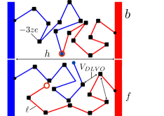
Figure 2: Coarse-Grained model of DNA strands tipped by reactive sites (circles). The squares represent the charges of the negative backbone that are coarsened (in groups of three) at the junction points of the chains and rescaled by a normalisation factor ($z$) that is provided by DLVO theory.Hansen and McDonald (1990)

III DNA-Coated Colloids

In this section we utilise tCBMC to compute the hybridisation free energy associated to bridge formation in DNACC systems (Fig. 2) and compare the results with previous attempts.Mognetti et al. (2012); Varilly et al. (2012) We map a single–stranded DNA into a FJC Zhang, Zhou, and Ou-Yang (2001) with unit length segment equal to $\ell=1.25\,$nm. The unit length segment $\ell$ has been chosen comparing end-to-end distances with a more accurate model of the DNA strands.Ouldridge, Louis, and Doye (2011) Each segment represents three bases, resulting in an averaged distance between nucleotides compatible with the experimental results Mills and Hagerman (2004); Tinland et al. (1997) (0.43-0.5 nm). The negative charges of the backbones are then grouped at the junction point between two unit segments (Fig. 2). A similar model was used in Ref. Mladek et al., 2012. We consider the tethers studied by Rogers et al. Rogers and Crocker (2011) of a Poly(T) string of 65 nucleotides terminated by a reactive sequence. The interaction between two charges ($i$ and $j$) placed at distance $r_{ij}$ is provided by a screened potential as given by the DLVO theoryHansen and McDonald (1990)

$$V_{\mathrm{DLVO}}(r_{ij})={(ze)^{2}\over 4\pi\epsilon_{0}\epsilon_{R}}{\exp[-r_{ij}/\lambda_{D}]\over r_{ij}}\,$$ (8)

where $z$ is the effective charge correctionHansen and McDonald (1990)

$$z={\exp[a/\lambda_{D}]\over 1+a/\lambda_{D}}\,.$$ (9)

In Eq. 8 $\lambda_{D}$ is the Debye length,Hansen and McDonald (1990) and $\epsilon_{0}$ is the vacuum dielectric constant. In the implicit solvent representation of Eq. 9, $a$ is the excluded salt region which has been taken equal to $a=0.5\,$ nm.Zhang, Zhou, and Ou-Yang (2001) The temperature is fixed at $T=308\,$K,Hansen and McDonald (1990) $\epsilon_{R}=75$, and we used a monovalent salt concentration equal to 125 mM.Rogers and Crocker (2011) The free constructs are made of $N_{1}=N_{2}=$21 segments, while the hybridised chain is made of $N_{b}=N_{1}+N_{2}$ segments with fixed end–points. $H^{(b)}$ and $H^{(f)}$ are then given by the sum over all the pairs of charges of the DLVO interaction (Eq. 8) augmented by the impermeable wall term. Notice that the end–points of the free chains also carry a charge and that the charge on the middle point of the bound construct is doubled. The excluded wall term constrains the constructs to remain within two parallel planes placed at distance $h$ (Fig. 2). Below, we consider the case in which the two tethering points are positioned opposite each other (i.e. on a line perpendicular to the two surface planes) and do not move along the surface.

Simulations are developed following the scheme presented in the previous sections. In each MC cycle, we either attempt to change topology (with 20% probability) or we implement a “standard” MC move (with 80% probability). The change-of-topology movement attempts to hybridise or to free a bound state with equal probability. When attempting to make (open) a bridge if the state is in the bound (free) state the MC move is rejected. “Standard” MC moves consist either in regrowing full chains using CBMC (with 20% probability) or in local rotations of chain branches by mean of pivot and double pivot MC moves. The swap between free and bound states is done as described in the previous section using the acceptance rules given by Eq. LABEL:acceptances. The hybridisation free energy is then computed using Eq. 7 by counting the number of times that bound and free states have been visited.

It is convenient to bias the run to explore a comparable number of bound and free configurations. This can be done by using a free energy bias $\Delta G_{\mathrm{bias}}$ that pushes the simulation, say, toward bound states. On the fly we can then iteratively correct $\Delta G_{\mathrm{bias}}$ by a factor $\log({\tilde{L}_{b}/\tilde{L}_{f}})$ (where $\tilde{L}_{b/f}$ is the number of times that the Markov chain has visited the bound/free state starting from the last time that $\Delta G_{\mathrm{bias}}$ has been corrected) until convergence where $\Delta G_{\mathrm{bias}}=\Delta G_{\mathrm{hyb}}$.

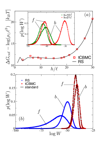
Figure 3: ($a$) $\Delta G_{\mathrm{cnf}}$ as a function of the plane distance calculated using Rosenbluth runsMognetti et al. (2012); Varilly et al. (2012) (full lines) and using the new proposed algorithm (red squares). Inset: distribution functions of the Rosenbluth weights generated in the tCBMC runs for $h/\ell=10$ and $h/\ell=21$. ($b$) Distribution functions of the Rosenbluth weight for $h=10\ell$ as obtained in Rosenbluth sampling (RS), in tCBMF, and in “standard” MC moves. In part $(b)$ and in the inset of part $(a)$, $f$ and $b$ label free and bound constructs.

Fig. 3$a$ (symbols) shows the results for $\Delta G_{\mathrm{cnf}}$ (Eq. 7) at different plane-to-plane distances $h$ (Fig. 2). Notice that the configurational free energy cost $\Delta G_{\mathrm{cnf}}$ has been translated by $k_{B}T\log(\rho_{\ominus}\ell^{3})$. This factor appears (along with $\Delta G_{0}$) as a pre–factor in the acceptance rules in Eq. LABEL:acceptances (notice thatTreloar (1946); Yamakawa (2001) $p\sim\ell^{-3}$). If compared with the static Rosenbluth method of Refs. Mognetti et al., 2012; Varilly et al., 2012 (full lines) the agreement is perfect (within the scattering due to the noise). In the inset of Fig. 3$a$ we report the probability distribution function of the Rosenbluth weight ($W$) of $f$ and $b$ constructs recorded using tCBMC. While for $h=10\ell$ we have overlap between the free and the bound distributions, for $h=21\ell$ the overlap region is minimal. Nevertheless convergence is achieved also in the latter case. This proves the robustness of the method and highlights the importance of using a bias ($\Delta G_{\mathrm{bias}}$) to record a sufficiently high number of jumps between $f$ and $b$ states.

To better highlight the different nature of the proposed method with respect to previous studies,Mognetti et al. (2012); Varilly et al. (2012) in Fig. 3$b$ we compare the Rosenbluth weights distributions obtained in the simulation of Fig. 3$a$ for $h=10\ell$ with those obtained in Rosenbluth sampling.Mognetti et al. (2012); Varilly et al. (2012) As expected,Batoulis and Kremer (1988); Mooij and Frenkel (1994) we find that the distributions of the static runsMognetti et al. (2012); Varilly et al. (2012) are very different from the distributions obtained with tCBMC. Moreover two different equilibrium runs (in which jumps between free and bound states were forbidden) provide the same distributions as tCBMC (full lines in Fig. 3). This confirms that tCBMC is indeed an equilibrium run. If this validates tCBMC from a technical perspective, we believe that the strength of the method, as compared to static approaches, lies in its versatility. This is illustrated in the next section.

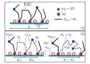
Figure 4: A system of polymers functionalized by receptors targeting a surface decorated by ligands:Dubacheva et al. (2014) $(a)$ definition of the model parameters, and $(b)$ loop inserting/deleting MC moves.

IV Adsorbed polymers

In this section we want to demonstrate how tCBMC can handle situations in which the typical configurations include a large number of different topologies separated by entropic barriers that cannot be easily overcome by standard simulations. We will study a system of polymers functionalized by receptors targeting a surface decorated by ligands (Fig. 4$a$). Most of the studies on polymer binding to surface (e.g. Ref. Eisenriegler, Kremer, and Binder, 1982; De Virgiliis et al., 2012; Daoud, 1991; Netz and Andelman, 2003) have focused on non–selective adsorption in which each monomer of the chain interacts with every element of the surface. Here, we consider the case in which a selected fraction of the monomers carries a binding site (receptor) whereas all other monomers cannot bind to the surface. Moreover, the surface is considered to display discrete binding sites (ligands) at a given surface density (Fig. 4). In this case the adsorbed chain can neatly be decomposed into a series of loops encompassed by two tails (Fig. 4). The selective–monomer case is usually addressed by standard simulationsBehringer and Gemünden (2013) or using theoretical modelling.Balazs, Singh, and Zhulina (1998); Cao and Wu (2005)

In this section we provide a valuable alternative by using the algorithm of Sec. II to design MC moves that allow to create/destroy loops in one go. We will use this algorithm to calculate the density of states ($\Omega(m)$) of adsorbed constructs which we define as

$$Z_{\mathrm{ads}}=\sum_{m\geq 1}Z(m) Z(m)=\Omega(m)\Big{[}{e^{-\beta\Delta G_{0}}\over\rho_{\ominus}}\Big{]}^{m}$$ (10)

where $Z_{\mathrm{ads}}$ ($Z(m)$) is the partition function of an adsorbed chain (binding $m$ ligands), and $\Delta G_{0}$ is the free-energy of the receptor–ligand dimerisation. We will compare our findings with the results of a mean field theory that will be developed to rationalise recent findings,Dubacheva et al. (2014) and that has been detailed in Appendix A. Our methodology has the potential to unveil how the typical configurations of the adsorbed chain affect the thermodynamics of adsorption.Dubacheva et al. (2014) This is more complicated than the case of functionalized nano–particles for which the configurational costs are simply additive in the number of bound tethers.Martinez-Veracoechea and Frenkel (2011)

The system of Fig. 4$a$ has been motivated by recent experiments on constructs of the biological polysaccharide hyaluronan (HA) functionalized with hosts reacting with guests immobilised on a surface.Dubacheva et al. (2014) HA have an unusually large Kuhn segment length,Attili, Borisov, and Richter (2012) and were here modelled by non-interacting FJCs made of $N_{\mathrm{seg}}=64$ segments of length $a_{K}=14\,$nm. On a FJC we randomly distribute $n_{R}$ receptors placed at the junction points between two segments (notice we have $N_{\mathrm{seg}}+1$ available spots). Each receptor can selectively bind a surface on which ligands are randomly distributed at a density equal to $1/d_{\ell}^{2}$, where $d_{\ell}$ is the averaged distance between ligands. In this study we have used $n_{R}=27$.Dubacheva et al. (2014) Each topology is characterised by a number $m$ of formed ligand-receptor complexes (Fig. 4$a$).

The tCBMC scheme employed is depicted in Fig.  4$b$. A loop is generated/destroyed as a result of the binding/unbinding of a randomly chosen receptor to/from a randomly chosen ligand. Such a scheme requires the ability to generate loop configurations with fixed end–points ($c_{ab}$ in Fig. 4$b$) and double–loop configurations with three fixed point constraints ($c_{a,b}$ in Fig. 4$b$). Notice that in Fig. 4$b$, $c_{ab}$ differs from $c_{a,b}$ only for the dashed parts of the chains. The remaining fraction of the polymer (full lines) is not affected by a single step implementation of the MC move and may include more loops. We generate configurations of type $c_{a,b}$ and $c_{ab}$ using the same procedure outlined in Sec. II. In particular when growing a loop of length $N_{a}$, we use the FJC end–to–end probability distribution function $p(|{\bf x}_{i-1}+{\bf u}_{i,\alpha}-{\bf r}_{a}|,N_{a}-i)$Treloar (1946); Yamakawa (2001) to generate trial vectors that are then sampled using the corresponding Rosenbluth weights (Sec. II). Here ${\bf x}_{i-1}$ is the end point of the $(i-1)$–th segment relative to the starting point of the loop. With such a procedure we can (re)grow single and double loop configurations and calculate their Rosenbluth weight (that we label by $W^{(a,b)}$ and $W^{(ab)}$ to distinguish between the two different topologies).

Given the previous procedure of generating configurations, the algorithm works as follows. When making a loop we attempt a reaction between a random receptor (chosen within the $m_{R,f}$ free ones) on the polymer and a random ligand (chosen within the $m_{\ell,f}$ ones that are free) on the surface (see Fig. 4). We then grow a new configuration of type $c^{(n)}_{a,b}$ and calculate the corresponding Rosenbluth weights $W^{(a,b)}(c^{(n)}_{a,b})$. Similarly, we retrace the old configuration $c^{(o)}_{ab}$ and calculate its Rosenbluth weight $W^{(ab)}(c^{(o)}_{ab})$. In the reverse move we try to un–bind a host–guest complex randomly chosen within the $m$ that are present in the system (Fig. 4$a$). Similarly to what was done before, we grow a new single loop configuration $c^{(n)}_{ab}$, (re)grow the current double-loop configuration ($c^{(o)}_{a,b}$), and measure the corresponding Rosenbluth weight ($W^{(ab)}(c^{(n)}_{ab})$ and $W^{(ab)}(c^{(o)}_{a,b})$). The acceptance rules for the two moves are then given by

$$acc_{ab\to a,b} = \mathrm{min}\Big{[}1,{m_{R,f}m_{\ell,f}\over m+1}{e^{-\beta\Delta G_{0}}\over\rho_{\ominus}}\cdot$$

$$\cdot{W^{(a,b)}(c^{(n)}_{a,b})\over W^{(ab)}(c^{(o)}_{ab})}{p(|{\bf r}_{a}|,N_{a})p(|{\bf r}_{b}|,N_{b})\over p(|{\bf r}_{a}+{\bf r}_{b}|,N_{a}+N_{b})}\Big{]}$$

$$acc_{a,b\to ab} = \mathrm{min}\Big{[}1,{m\over(m_{R,f}+1)(m_{\ell,f}+1)}{\rho_{\ominus}\over e^{-\beta\Delta G_{0}}}\cdot$$

$$\cdot{W^{(ab)}(c^{(n)}_{ab})\over W^{(a,b)}(c^{(o)}_{a,b})}{p(|{\bf r}_{a}+{\bf r}_{b}|,N_{a}+N_{b})\over p(|{\bf r}_{a}|,N_{a})p(|{\bf r}_{b}|,N_{b})}\Big{]}\,.$$

We recognise that the structure of Eqs. IV and IV is the same as that of Eqs. LABEL:acceptances (with $W^{(a,b)}$ and $W^{(ab)}$ replacing $W^{(f)}$ and $W^{(b)}$ respectively). The pre–factors are due to the fact that, following the flow of the algorithm, the probability to generate a $c^{(n)}_{a,b}$ or a $c^{(n)}_{ab}$ configuration is equal to $1/(m_{R,f}m_{\ell,f})$ and $1/m$ respectively.

Notice that the randomly selected reacting receptor could be on the tail of the construct (rather than in a loop as in Fig. 4$b$). In this case the algorithm should sample between a configuration made of a tail and a configuration made of a tail plus a loop. This can be easily implemented by generalising the way configurations are generated and Eqs. IV and IV. For completeness, we detail how the algorithm works in this case in Appendix B.

We also report that more efficient runs were obtained by implementing a MC move that re–arranges two loops by swapping the ligand which a receptor is bound to. The details are also reported in Appendix B. Notice that such a move would be required to guarantee the ergodicity of the algorithm in the case that the choice of the free ligand to bind/unbind (when making/destroying a loop) would be restricted (for efficiency purposes) to a region enclosing the tethering points. In that case certain loops with stretched strands could be unreachable by an algorithm that would only use making/destroying loop moves. Alternatively one can think of biasing the choice of the ligands in more subtle ways that also depend on the length of the loops/tails that encompass the randomly selected receptor, as well as on the positions of the ligands to whom such loops/tails are tethered. Those complications were avoided in our current study. In particular, we randomly distributed ligands across a square of side $L=11\cdot a_{K}$ with periodic boundary conditions and, when attempting to bind/unbind receptors, the ligands were chosen uniformly.

We are now in a position to sample between the different topologies of an adsorbed polymer by adding and removing loops. This could be hampered by high free energy barriers resulting in runs exploring only a very few distinct $m$. To avoid this kind of trapping, we have used the successive umbrella sampling (SUS) scheme of Virnau and Müller.Virnau and Müller (2004) At a certain step of the simulation we only allow sampling between configurations with $m$ and $m-1$ attached receptors. This implies that if the system is in a state with $m$ ($m-1$ receptors) and we attempt to create (destroy) a loop the MC move is immediately rejected. By sequentially moving the window within which the sampling is constrained, we can reconstruct $Z(m)$ by usingVirnau and Müller (2004)

$$\alpha_{m}={\Omega(m)\over\Omega(m-1)}={N_{m}\over N_{m-1}} {\Omega(m)\over\Omega(1)}=\prod_{i=2}^{m}\alpha_{m}\,,$$ (13)

where $N_{m}$ and $N_{m-1}$ are the number of times that the run has visited a configuration with $m$ and $m-1$ complexes formed when constrained between $m-1$, and $m$.

Figure 5: Density of states versus number of bound receptors at different ligand concentrations (the arrow direction points toward data sets with higher $d_{\ell}$). In part $(a)$ $\Omega(m)$ is reported in simulation units while in $(b)$ we test the mean field scaling prediction of Eq. 14 (full line).

In Figure 5$a$ we report the density of states $\Omega(m)$ (Eqs. 13 and 10) normalised by $\Omega(1)$. While increasing the average ligand–ligand distance $d_{\ell}$, $\Omega(m)$ decreases. Interestingly, in intermediate regions, $\Omega(m)$ exhibits a maximum.

This finding is easily interpreted. $\Omega(m)$ is the result of the competition between the combinatorial gain of many ligands that can bind many receptors and the configurational cost associated to the formation of loops and to the polymer surface interaction (Fig. 4).Note1 (b) Increasing the ligand density (i.e. decreasing $d_{\ell}$) rises the multivalency of the system, and the density of states increases because of the combinatorial gain.

This statement can be made more rigorous considering a MF theory in which ligands are regularly distributed with a homogeneous density $1/d_{\ell}^{2}$. We can show that in this approximation (see Appendix A) the partition function can be written as

$$\Omega_{\mathrm{MF}}(m) = n_{\ell}\Big{[}{\sqrt{3/2\pi}\over d_{\ell}^{2}a_{K}}\Big{]}^{m-1}\Psi(m)\,,$$ (14)

where $\Psi(m)$ is a function that only depends on the architecture of the functional chain (see Eq. LABEL:eq:Psi), and $n_{\ell}$ is the number of ligands present on the plane. In particular $\Psi$ accounts for the multivalency of the receptors on the chain but is independent of $d_{\ell}$. Interestingly Eq. 14 predicts a scaling relation between $\Omega$ and $d_{\ell}$ that has been tested in Fig. 5$b$ for the simulation results of Fig. 5$a$. Satisfactorily, when plotting $\Omega(m)d_{\ell}^{2(m-1)}$ we find a nice collapse of the density of states at different ligand concentrations. Importantly at small $d_{\ell}$ simulations agree with the MF theory. This is not the case when $d_{\ell}$ becomes comparable with the length of the Kuhn segment $a_{K}$. Indeed in this case the typical loop configurations become more stretched, resulting in a density of states smaller than what is predicted by the MF theory. Overall, the results of this section validate the use of tCBMC to study selective adsorption of polymers, the key advantage being the possibility to sample directly between different adsorbed states by means of dedicated MC moves.

V Discussions

Functionalizing complex macromolecules by reactive elements is nowadays a popular tool to engineer self–assembling systems and smart aggregates. In spite of the high degree of designability of these materials, efficient simulation methods are hampered by the multi–scale nature of these systems.

In this paper we have developed a Monte Carlo scheme dedicated to the study of thermally reconfigurable supramolecular networks. This scheme combines an implicit treatment of the reactive sites with coarse grained simulations that are used to sample the polymeric network. Based on our previous works,Mognetti et al. (2012); Varilly et al. (2012) and similar to what is done in existing literature,Chen and Escobedo (2000); Vendruscolo (1997); Dijkstra, Frenkel, and Hansen (1994); Wick and Siepmann (2000) we have used schemes that can generate polymers whose configurations are constrained by the reactions of the active spots. Comparably to what is done in configurational bias MC,Siepmann and Frenkel (1992) we use the bias measured while generating these configurations to implement dynamic MC moves between them. The novel development in the present case is that we were able to directly sample between states with different topologies.

First we tested the algorithm by considering tethered constructs tipped by reactive spots as in systems of DNA coated colloids. We have demonstrated that the proposed method can reproduce the correct hybridisation free energy previously obtained using established methods.

We have then studied a system of polymers functionalized by receptors binding ligands distributed on a surface. In this case many possible topologies are present, with polymers exhibiting multiple loops while binding different groups of receptors to different groups of ligands. Such topologies are separated by entropic barriers that hamper the efficiency of algorithms based on local Monte Carlo moves. We have demonstrated the ability of the proposed algorithm to handle also this system, supporting the usefulness of the proposed method with respect to existing techniques. This has been done by measuring the density of states of adsorbed chains and by comparing them to the predictions of a mean field theory. In appendix A we show how this quantity can be used to derive, e.g., binding isotherms and to identify regions in parameter space where the functionalized constructs discriminate sharply between surfaces with high and low ligand coverage.Martinez-Veracoechea and Frenkel (2011); Dubacheva et al. (2014) This “superselective” behaviour is desirable when engineering smart systems for drug delivery.

We believe that the proposed method could support the understanding and the design of supramolecular systems. For instance, concerning DNA coated colloids, it will allow to calculate the full density of states of two particles cross-linked by a given number of bridges. This will highlight the role played by tether–tether interactions which is usually neglected in the modelling of micron-sized particlesRogers and Crocker (2011); Mognetti et al. (2012); Varilly et al. (2012) but which has been shown to be relevant for particles of sub-micron size.Mladek et al. (2012) Concerning selective targeting, the proposed method could aid the design of functionalized chains resulting in desired properties. In this respect, it will be important to generalise our scheme to worm-like chain models and study how the ligand–receptor affinity is altered when the receptor is mounted on a semi–flexible segment.Hsu and Binder (2013) This can be done in view of the fact that it is possible to grow fixed end–point chains featuring strong intramolecular interactions between adjacent segments of the chains.Wick and Siepmann (2000) The study of excluded volume interactions between polymers is also desirable. In a more general perspective, it will be interesting to explore the usefulness of the method when applied to other relevant systems like, for instance, network forming polymers.Dimopoulos et al. (2010); Biffi et al. (2013); Schmid (2013); Stals et al. (2014) This will deserve future investigations.

Acknowledgements. Computational resources were kindly provided by the HCP Computer Center of the ULB/VUB (Brussels), and by the “Consortium des Equipements pour le Calcul Intensif” (CECI). We acknowledge Oleg Borisov for fruitful discussions concerning the mean field theory of adsorbed chains. T.C. acknowledges support from the Herchel Smith fund. G.V.D. acknowledges Marie Curie Career Integration Grant CELLMULTIVINT (PCIG09-GA-2011-293803).

Appendix A A Mean Field Theory for Adsorbed Chains

In this appendix we derive the mean field estimate that has been used in section IV to compare the partition function of an adsorbed polymer $Z(m)$ (Eq. 14 and Fig. 5). This is possible in view of the fact that we are taking ideal constructs for which the partition function of an adsorbed chain can be decomposed into the product of loops and tails.

We first concentrate on calculating the partition function of a tail made of $n$ segments ($Z_{\mathrm{tail}}(n)$) and the partition function of a loop made of $n$ segments with end points tethered at a distance equal to $r$ ($Z_{\mathrm{loop}}(n;r)$). By means of Rosenbluth sampling we obtain

$$Z_{\mathrm{tail}}(n)\approx{0.55\over\sqrt{n}} n\geq 1\,,$$

$$Z_{\mathrm{loop}}(n;r)={p(r,n)\over n} n\geq 2\,.$$ (15)

$Z_{\mathrm{tail}}$ and $Z_{\mathrm{loop}}$ are calculated with respect to the partition function of an ideal chain of length $n$ and fixed starting point. In particular, in Eq. 15 the $1/\sqrt{n}$ and $1/n$ terms are the corrections due to the impermeability of the plane, while the end point constraint in $Z_{\mathrm{loop}}$ is accounted for by the distribution function $p(r,n)$.Treloar (1946); Yamakawa (2001) We define by $x_{i}$ ($i=1,\cdots,n_{R}$) the ordered sequence of the positions of the receptors along the chain ($x_{i}\in[0,\cdots,N_{\mathrm{seg}}]$ with $x_{i}<x_{j}$ if $i<j$).

Using Eq. 15 we can compute the partition function of a chain binding $m$ ligands (placed in ${\bf r}_{\alpha}$, $\alpha=1,\cdots,m$) to the $m$ receptors $x_{\sigma_{\alpha}}$ (where $\sigma_{\alpha}<\sigma_{\beta}$ if $\alpha<\beta$):

$$Z(\{x_{\sigma_{\alpha}},{\bf r}_{\alpha}\}) = Z_{\mathrm{tail}}(x_{\sigma_{1}})Z_{\mathrm{tail}}(N_{\mathrm{seg}}-x_{\sigma_{m}})\Big{[}{e^{-\beta\Delta G_{0}}\over\rho_{\ominus}}\Big{]}^{m}\cdot$$

$$\cdot\prod_{\alpha=2}^{m}Z_{\mathrm{loop}}(|{\bf r}_{\alpha}-{\bf r}_{\alpha-1}|,x_{\sigma_{\alpha}}-x_{\sigma_{\alpha-1}}).$$

In the previous expression $\sigma$ labels one of the $n_{R}!/(m!(n_{R}-m)!)$ different sets of $m$ receptors taken from the $n_{R}$ ones present on the chain.

Next we approximate the end–to–end distribution function in Eq. 15 with a Gaussian

$$p(r,n)\approx\Big{(}{3\over 2na_{K}^{2}\pi}\Big{)}^{3/2}\exp\Big{[}-{3r^{2}\over 2a_{K}^{2}n}\Big{]}\,.$$ (17)

Although this is a good approximation only when $n$ is large we have verified, using the explicit form of the end–to–end distance $p(r,n)$,Treloar (1946); Yamakawa (2001) that the relative discrepancy in the final result is always smaller than $2\%$ (data not shown).

We now approximate the ligand positions $\{{\bf r}_{i}\}$ by a homogeneous distribution of density $1/d_{\ell}^{2}$. Practically this allows to replace sums into integrals as follows

$$\sum_{\{{\bf r}_{\alpha}\}}\Big{[}\cdot\Big{]}=\Big{[}{1\over d_{\ell}^{2}}\Big{]}^{m}\int\mathrm{d}{\bf r}_{1}\cdots\mathrm{d}{\bf r}_{m}\Big{[}\cdot\Big{]}\,.$$ (18)

Using Eqs. 18, 15, and 17 into Eq. LABEL:Zmr we can calculate the partition function of a chain adsorbed by the receptors $x_{\sigma_{\alpha}}$ ($\alpha=1,\cdots,m$)

$$Z(\{x_{\sigma_{\alpha}}\})\approx\sum_{\{{\bf r}_{i}\}}Z(\{x_{i},{\bf r}_{i}\})=n_{\ell}\Big{[}{e^{-\beta\Delta G_{0}}\over\rho_{\ominus}}\Big{]}^{m}\Big{[}{\sqrt{3/2\pi}\over d_{\ell}^{2}a_{K}}\Big{]}^{m-1}$$

$$\cdot{0.55^{2}}\sqrt{1\over x_{\sigma_{1}}(N_{\mathrm{seg}}-x_{\sigma_{m}})}\prod_{i=2}^{m}\Big{[}{1\over x_{\sigma_{i}}-x_{\sigma_{i-1}}}\Big{]}^{3/2}$$

(19)

where $n_{\ell}$ is the number of ligands present on the plane which is taken to be a square of side length equal to $11\cdot a_{K}$ (see Sec. IV). Finally summing over all the possible sets of $m$ receptors ($\sigma$) we obtain $Z(m)$ as defined in Sec. IV:

$$Z(m) = \sum_{\sigma}Z(\{x_{\sigma_{\alpha}}\})$$ (20)

$$= n_{\ell}\Big{[}{e^{-\beta\Delta G_{0}}\over\rho_{\ominus}}\Big{]}^{m}\Big{[}{\sqrt{3/2\pi}\over d_{\ell}^{2}a_{K}}\Big{]}^{m-1}\Psi(m)$$

$$\Psi(m) = \sum_{\sigma}{0.55^{2}}\sqrt{1\over x_{\sigma_{1}}(N_{\mathrm{seg}}-x_{\sigma_{m}})}\prod_{i=2}^{m}\Big{[}{1\over x_{\sigma_{i}}-x_{\sigma_{i-1}}}\Big{]}^{3/2}$$

$\Psi(m)$ only depends on the position of the receptors on the chain and has been computed by an exact enumeration. In particular for the results of Fig. 5 the 27 receptors were placed at the position $\{x_{i}\}=\{$2, 3, 5, 7, 10, 14, 15, 19, 23, 29, 31, 34, 35, 36, 39, 44, 48, 50, 51, 54, 55, 56, 57, 59, 60, 61, 62$\}$ along the $N_{\mathrm{seg}}+1=65$ possible positions. Notice that although we have 27 receptors, In Fig. 5 we never observed more than $m=19$ complexes reacting. This is due to the fact that receptors that are at the two extremities of the same segment were never allowed to bind simultaneously. Indeed a concurrent reaction would over–constrain the system. Other ways of distributing receptors on the chains (e.g. forbidding neighbouring receptors) did not alter the general picture.

Figure 6: Number of polymers adsorbed per unit area ($\Gamma$) and selectivity parameter ($\alpha$) as a function of the scaling parameter $y$ at two different concentrations.Dubacheva et al. (2014)

Using the density of states we can calculate the binding isotherms. In particular, following the modelling presented in Ref. Dubacheva et al., 2014, we divide the functionalized plane into square cells of side size equal to $a$. Limiting our study to the case in which no more than a single polymer can bind a cell, the partition function of a polymer adsorbed onto a cell is given by $Z(m)$ (Eq. 20) with

$$n_{\ell}={a^{2}\over d_{\ell}^{2}}\,.$$ (22)

This scenario is simplified with regard to the real system but has been chosen because it is illustrative. By equalising the chemical potential of a polymer in the bulk with the chemical potential of an adsorbed polymer, we can easily calculate the fraction of cells ($\Theta$) that are occupied by a polymer. In particular if we define

$$Z_{\mathrm{bnd}} = c\sum_{m}Z(m)=ca^{2}a_{K}\sum_{m}y^{m}\Psi(m)$$ (23)

where $c$ is the bulk concentration of the polymers and $y$ is the following scaling variable

$$y = {\exp[-\beta\Delta G_{0}]\sqrt{3/2\pi}\over d_{\ell}^{2}a_{K}\rho_{\ominus}}$$ (24)

we find

$$\Theta={Z_{\mathrm{bnd}}\over Z_{\mathrm{bnd}}+1}\,.$$ (25)

Using $\Theta$ we can then derive the number of adsorbed polymers per unit area

$$\Gamma={\Theta\over a^{2}}\,.$$ (26)

We notice that the leading term of $\Gamma$ when $y\to 0$ does not depend on $a$ ($\Gamma\sim ca_{K}\sum_{m}y^{m}\Psi(m)$).

Results for $\Gamma$ are reported in Fig. 6 (black curves, left $y$-axis), as a function of the scaling variable $y$ at two different polymer concentrations $c$. For a given polymer system, the scaling variable $y$ is proportional to the ligand surface density. Notice that the number of chains adsorbed increases with the scaling variable $y$. It is useful to calculate the selectivity parameter defined as Martinez-Veracoechea and Frenkel (2011)

$$\alpha = {\mathrm{d}\log\Gamma\over\mathrm{d}\log c_{\ell}}={\mathrm{d}\log\Gamma\over\mathrm{d}\log y}$$ (27)

where $c_{\ell}=1/d_{\ell}^{2}$ is the density of ligands. Notice that $\alpha$ measures how sensible the adsorption process is to a change in the ligand surface density. Calculated values for $\alpha$ are reported in Fig. 6 (red curves, right $y$-axis). The superselective region is characterised by $\alpha>1$ and follows previously reported trend.Martinez-Veracoechea and Frenkel (2011); Dubacheva et al. (2014) However, at this point, a quantitative agreement with experiments is still missing.Dubacheva et al. (2014) This is related to limitations of the coarse-grained model for the polymer (that, e.g., neglects chain rigidity close to a receptor) and to the fact that we did not allow multiple polymers binding to the same lattice site in the adsorbed phase. These aspects go beyond the scope of this paper and will be addressed elsewhere.

Figure 7: MC moves by which a receptor on the tail bind/unbind from a ligand $(a)$ and by which a receptor changes ligand to which is bound $(b)$.

Appendix B Tail Reactions and Ligand Swapping

In this section we complete the description of the MC moves introduced in Sec. IV. First we consider the reaction of a receptor on a tail (Fig. 7$a$). In this case we have to sample between a tail $c_{ab}$ and a tail plus a loop $c_{a,b}$ (dashed lines in Fig. 7$a$). The generation of the loop follows what was done in Sec. IV. The tail can be generated in the same way as the free constructs in the DNA system (Sec. III). In particular the trial segments are not biased by the end-to-end distribution function $p$ but are generated with a uniform distribution. Using the notation of Sec. IV, the acceptance rules are then given by

$$acc_{ab\to a,b} = \mathrm{min}\Big{[}1,{m_{R,f}m_{\ell,f}\over m+1}{e^{-\beta\Delta G_{0}}\over\rho_{\ominus}}\cdot$$

$$\cdot{W^{(a,b)}(c^{(n)}_{a,b})\over W^{(ab)}(c^{(o)}_{ab})}p(|{\bf r}_{b}|,N_{b})\Big{]}$$

$$acc_{a,b\to ab} = \mathrm{min}\Big{[}1,{m\over(m_{R,f}+1)(m_{\ell,f}+1)}\cdot$$

$$\cdot{\rho_{\ominus}\over e^{-\beta\Delta G_{0}}}{W^{(ab)}(c^{(n)}_{ab})\over W^{(a,b)}(c^{(o)}_{a,b})}{1\over p(|{\bf r}_{b}|,N_{b})}\Big{]}\,.$$

We now consider the swapping of a ligand (Fig. 7$b$). In this case a bound receptor is detached and rebound to another ligand. This implies the construction of double loop configurations ($c_{a,b}$) that is done as described in Sec. IV. The acceptance of the receptor displacement is then given by (see Fig. 7)

$$acc_{a,b\to a,b} = \mathrm{min}\Big{[}1,{W^{(a,b)}(c^{(n)}_{a,b})\over W^{(a,b)}(c^{(o)}_{ab})}{p(|{\bf r}^{\prime}_{a}|,N_{a})p(|{\bf r}^{\prime}_{b}|,N_{b})\over p(|{\bf r}_{a}|,N_{a})p(|{\bf r}_{b}|,N_{b})}\Big{]}$$

The previous acceptance rule is slightly modified when the receptor that is moved is the tethering point of one of the two tails. In this case we have to sample between configurations made of a loop plus a tail.

References

- Note1 (a) Author to whom correspondence should be addressed. Electronic mail: bmognett@ulb.ac.be.
- Mirkin et al. (1996) C. A. Mirkin, R. L. Letsinger, R. C. Mucic, J. J. Storhoff, et al., “A dna-based method for rationally assembling nanoparticles into macroscopic materials,” Nature 382, 607 (1996).
- Alivisatos et al. (1996) A. P. Alivisatos, K. P. Johnsson, X. Peng, T. E. Wilson, C. J. Loweth, M. P. Bruchez, and P. G. Schultz, “Organization of ’nanocrystal molecules’ using dna,” Nature 382, 609 (1996).
- Di Michele and Eiser (2013) L. Di Michele and E. Eiser, “Developments in understanding and controlling self assembly of dna-functionalized colloids,” Phys. Chem. Chem. Phys. 15, 3115 (2013).
- Dubacheva et al. (2014) G. V. Dubacheva, T. Curk, B. M. Mognetti, R. Auzély-Velty, D. Frenkel, and R. P. Richter, “Superselective targeting using multivalent polymers,” J. Am. Chem. Soc. 136, 1722 (2014).
- Kiessling and Grim (2013) L. L. Kiessling and J. C. Grim, “Glycopolymer probes of signal transduction,” Chem. Soc. Rev. 42, 4476 (2013).
- Han et al. (2011) D. Han, S. Pal, J. Nangreave, Z. Deng, Y. Liu, and H. Yan, “Dna origami with complex curvatures in three-dimensional space,” Science 332, 342 (2011).
- Biffi et al. (2013) S. Biffi, R. Cerbino, F. Bomboi, E. M. Paraboschi, R. Asselta, F. Sciortino, and T. Bellini, “Phase behavior and critical activated dynamics of limited-valence dna nanostars,” P. Natl. Acad. Sci. U.S.A. 110, 15633 (2013).
- Schmid (2013) F. Schmid, “Self-consistent field approach for cross-linked copolymer materials,” Phys. Rev. Lett. 111, 028303 (2013).
- Martinez-Veracoechea and Frenkel (2011) F. J. Martinez-Veracoechea and D. Frenkel, “Designing super selectivity in multivalent nano-particle binding,” P. Natl. Acad. Sci. U.S.A. 108, 10963 (2011).
- Dreyfus et al. (2010) R. Dreyfus, M. E. Leunissen, R. Sha, A. Tkachenko, N. C. Seeman, D. J. Pine, and P. M. Chaikin, “Aggregation-disaggregation transition of dna-coated colloids: Experiments and theory,” Phys. Rev. E 81, 041404 (2010).
- Leunissen and Frenkel (2011) M. E. Leunissen and D. Frenkel, “Numerical study of dna-functionalized microparticles and nanoparticles: Explicit pair potentials and their implications for phase behavior,” J. Chem. Phys. 134, 084702 (2011).
- Mognetti, Leunissen, and Frenkel (2012) B. M. Mognetti, M. E. Leunissen, and D. Frenkel, “Controlling the temperature sensitivity of dna-mediated colloidal interactions through competing linkages,” Soft Matter 8, 2213 (2012).
- Mognetti et al. (2012) B. M. Mognetti, P. Varilly, S. Angioletti-Uberti, F. J. Martinez-Veracoechea, J. Dobnikar, M. E. Leunissen, and D. Frenkel, “Predicting DNA-mediated colloidal pair interactions,” P. Natl. Acad. Sci. U.S.A. 109, E378 (2012).
- Varilly et al. (2012) P. Varilly, S. Angioletti-Uberti, B. M. Mognetti, and D. Frenkel, “A general theory of dna-mediated and other valence-limited colloidal interactions,” J. Chem. Phys. 137, 094108 (2012).
- Angioletti-Uberti et al. (2013) S. Angioletti-Uberti, P. Varilly, B. M. Mognetti, A. V. Tkachenko, and D. Frenkel, “Communication: A simple analytical formula for the free energy of ligand–receptor-mediated interactions,” J. Chem. Phys. 138, 021102 (2013).
- Ouldridge, Louis, and Doye (2011) T. E. Ouldridge, A. A. Louis, and J. P. Doye, “Structural, mechanical, and thermodynamic properties of a coarse-grained dna model,” J. Chem. Phys. 134, 085101 (2011).
- Rogers and Crocker (2011) W. B. Rogers and J. C. Crocker, “Direct measurements of dna-mediated colloidal interactions and their quantitative modeling,” P. Natl. Acad. Sci. U.S.A. 108, 15687 (2011).
- Frenkel and Smit (2001) D. Frenkel and B. Smit, Understanding Molecular Simulation, 2nd ed. (Academic Press, Inc., Orlando, FL, USA, 2001).
- Mooij and Frenkel (1994) G. Mooij and D. Frenkel, “The overlapping distribution method to compute chemical potentials of chain molecules,” J. Phys.-Condens. Mat. 6, 3879 (1994).
- Batoulis and Kremer (1988) J. Batoulis and K. Kremer, “Statistical properties of biased sampling methods for long polymer chains,” J. Phys. A-Math. Gen. 21, 127 (1988).
- Siepmann and Frenkel (1992) J. I. Siepmann and D. Frenkel, “Configurational bias monte carlo: a new sampling scheme for flexible chains,” Mol. Phys. 75, 59 (1992).
- Virnau and Müller (2004) P. Virnau and M. Müller, “Calculation of free energy through successive umbrella sampling,” J. Chem. Phys. 120, 10925 (2004).
- Siepmann and McDonald (1992) J. I. Siepmann and I. R. McDonald, “Monte carlo simulations of mixed monolayers,” Molecular Physics 75, 255 (1992).
- Note (2) There are different ways of doing this. For instance, we can think of growing an entire chain before starting with the second one or we can grow the chains concurrently, by changing the chain to grow at each step of the algorithm. The optimal choice depends on the specific system that is investigated.
- Treloar (1946) L. R. G. Treloar, “The statistical length of long-chain molecules,” Rubber Chem. Technol. 19, 1002 (1946).
- Yamakawa (2001) H. Yamakawa, Modern Theory of Polymer Solutions (electronic edition, 2001).
- Chen and Escobedo (2000) Z. Chen and F. A. Escobedo, “A configurational-bias approach for the simulation of inner sections of linear and cyclic molecules,” J. Chem. Phys. 113, 11382 (2000).
- Vendruscolo (1997) M. Vendruscolo, “Modified configurational bias monte carlo method for simulation of polymer systems,” J. Chem. Phys. 106, 2970 (1997).
- Dijkstra, Frenkel, and Hansen (1994) M. Dijkstra, D. Frenkel, and J.-P. Hansen, “Phase separation in binary hard-core mixtures,” J. Chem. Phys. 101, 3179 (1994).
- Wick and Siepmann (2000) C. D. Wick and J. I. Siepmann, “Self-adapting fixed-end-point configurational-bias monte carlo method for the regrowth of interior segments of chain molecules with strong intramolecular interactions,” Macromolecules 33, 7207 (2000).
- Hansen and McDonald (1990) J.-P. Hansen and I. R. McDonald, Theory of simple liquids (Elsevier, 1990).
- Zhang, Zhou, and Ou-Yang (2001) Y. Zhang, H. Zhou, and Z.-C. Ou-Yang, “Stretching single-stranded dna: interplay of electrostatic, base-pairing, and base-pair stacking interactions,” Biophys. J. 81, 1133 (2001).
- Mills and Hagerman (2004) J. B. Mills and P. J. Hagerman, “Origin of the intrinsic rigidity of dna,” Nucleic Acids Res. 32, 4055 (2004).
- Tinland et al. (1997) B. Tinland, A. Pluen, J. Sturm, and G. Weill, “Persistence length of single-stranded dna,” Macromolecules 30, 5763 (1997).
- Mladek et al. (2012) B. M. Mladek, J. Fornleitner, F. J. Martinez-Veracoechea, A. Dawid, and D. Frenkel, “Quantitative prediction of the phase diagram of dna-functionalized nanosized colloids,” Phys. Rev. Lett. 108, 268301 (2012).
- Eisenriegler, Kremer, and Binder (1982) E. Eisenriegler, K. Kremer, and K. Binder, “Adsorption of polymer chains at surfaces: Scaling and monte carlo analyses,” J. Chem. Phys. 77, 6296 (1982).
- De Virgiliis et al. (2012) A. De Virgiliis, A. Milchev, V. Rostiashvili, and T. Vilgis, “Structure and dynamics of a polymer melt at an attractive surface,” Eur. Phys. J. E: Soft Matter and Biological Physics 35, 1 (2012).
- Daoud (1991) M. Daoud, “Adsorption of polymers,” Polym. J. 23, 651 (1991).
- Netz and Andelman (2003) R. R. Netz and D. Andelman, “Neutral and charged polymers at interfaces,” Phys. Rep. 380, 1 (2003).
- Behringer and Gemünden (2013) H. Behringer and P. Gemünden, “Homopolymer adsorption on periodically structured surfaces in systems with incommensurable lengths,” J. Chem. Phys. 138, 174905 (2013).
- Balazs, Singh, and Zhulina (1998) A. C. Balazs, C. Singh, and E. Zhulina, “Stabilizing properties of copolymers adsorbed on heterogeneous surfaces: a model for the interactions between a polymer-coated influenza virus and a cell,” Macromolecules 31, 6369 (1998).
- Cao and Wu (2005) D. Cao and J. Wu, “Theoretical study of cooperativity in multivalent polymers for colloidal stabilization,” Langmuir 21, 9786 (2005).
- Attili, Borisov, and Richter (2012) S. Attili, O. V. Borisov, and R. P. Richter, “Films of end-grafted hyaluronan are a prototype of a brush of a strongly charged, semiflexible polyelectrolyte with intrinsic excluded volume,” Biomacromolecules 13, 1466 (2012).
- Note1 (b) Notice that these contributions are neatly visible in the acceptance rules Eqs.IV IV.
- Hsu and Binder (2013) H.-P. Hsu and K. Binder, “Effect of chain stiffness on the adsorption transition of polymers,” Macromolecules 46, 2496 (2013).
- Dimopoulos et al. (2010) A. Dimopoulos, J.-L. Wietor, M. W bbenhorst, S. Napolitano, R. A. van Benthem, G. de With, and R. P. Sijbesma, “Enhanced mechanical relaxation below the glass transition temperature in partially supramolecular networks,” Macromolecules 43, 8664 (2010).
- Stals et al. (2014) P. J. Stals, M. A. Gillissen, T. F. Paffen, T. F. de Greef, P. Lindner, E. Meijer, A. R. Palmans, and I. K. Voets, “Folding polymers with pendant hydrogen bonding motifs in water: The effect of polymer length and concentration on the shape and size of single-chain polymeric nanoparticles,” Macromolecules (2014).