Multidomain spectral method for Schrödinger equations

Abstract.

A multidomain spectral method with compactified exterior domains combined with stable second and fourth order time integrators is presented for Schrödinger equations. The numerical approach allows high precision numerical studies of solutions on the whole real line. At examples for the linear and cubic nonlinear Schrödinger equation, this code is compared to transparent boundary conditions and perfectly matched layers approaches. The code can deal with asymptotically non vanishing solutions as the Peregrine breather being discussed as a model for rogue waves. It is shown that the Peregrine breather can be numerically propagated with essentially machine precision, and that localized perturbations of this solution can be studied.

1. Introduction

It is a common problem in the numerical treatment of partial differential equations (PDEs) that most of the PDEs appearing in applications are defined on $\mathbb{R}^{d}$ where $d$ is the dimension, i.e., on unbounded domains, whereas computers are generally able to deal with only finite domains. One popular approach in this context is to set up the problem on a finite domain and to impose transparent boundary conditions (TBC) which give the boundary data which would appear at this location if the initial value problem where treated on the whole $\mathbb{R}^{d}$, or artificial boundary conditions approximating TBC. To this end a certain relation between Dirichlet and von Neumann data at the boundary has to be satisfied called the Dirichlet to von Neumann map, see e.g. [15, 31] for reviews of TBC approaches and in particular [1] for Schrödinger equations. An alternative approach is given by perfectly matched layers (PML) which were introduced by Bérenger [5] for the Maxwell equations. The idea is to join absorbing layers at the boundaries of the computational domain. The to be solved PDE is deformed in the layers in a way that the solution in the computational domain is not affected, and that it is rapidly dissipated in the layers. This PML approach was adapted to various equations, see for instance [26, 16] for Schrödinger equations. We use here the approach [36] that is similar to exterior complex scaling methods [25].

An interesting approach to treat PDEs on unbounded domains is to map infinite domains to finite domains. In a numerical context, this was apparently first used in [27] and later for the Schrödinger equation in [22]. Whereas [22] uses a finite difference method, [27] incorporates one of the first applications of a spectral method with Chebyshev polynomials. A very efficient variant of the latter mainly used in astrophysics, see for instance [34], are multidomain methods with compactified exterior domains (CED). As in so called infinite element approaches, see for instance [14] for Schrödinger equations, the idea is to map the exterior domain with some Möbius transformation to a finite domain. In this paper, we apply a multidomain spectral approach with CED to Schrödinger equations and compare this to TBC and PML approaches for concrete examples. The CED method clearly needs more resolution in space, but it will be shown that it is competitive especially in the nonlinear case since the TBC have to be implemented iteratively and since the parameters of the PML have to be optimized through several runs of the code for the studied example. In addition CED are attractive if high precision is needed since PML do not appear to provide sufficient accuracy in the NLS cases studied here, and since TBC are often not known and have to be implemented approximately. CED methods on the contrary are shown to provide the same accuracy in the linear and nonlinear cases. Moreover the TBC and PML approaches here require compact support of the initial data in the computational domain whereas the CED approach just requires asymptotically bounded initial data and can even deal with an algebraic fall off of the solutions.

In the focus of this paper are Schrödinger equations of the form

(1) $$i\partial_{t}u+\partial_{xx}u+V(|u|^{2},x)u=0,$$

where $u=u(x,t):\mathbb{R}\times\mathbb{R}\mapsto\mathbb{C}$, and where the potential $V$ is either a function of $x$ only or of $|u|^{2}$. In concrete examples, we study the case of the free linear Schrödinger equation with $V=0$ and of the focusing cubic nonlinear Schrödinger equation (NLS) with $V=2|u|^{2}$. It is straight forward to generalize the presented CED and PML approaches to more general potentials $V$, whereas this requires more work for TBC. The importance of the linear Schrödinger equation needs hardly be stressed since it is the governing PDE of quantum mechanics. In addition it arises in many applications as in quantum semiconductors [7], in electromagnetic wave propagation [24], in seismic migration [12], as the lowest order one-way approximation (paraxial wave equation) to the Helmholtz equation, under the notion of Fresnel equation in optics [29], or in underwater acoustics [30]. But also the NLS equations appear in many applications in hydrodynamics, nonlinear optics and Bose-Einstein condensates mainly in the description of the modulation of waves. The cubic NLS which we study here in more detail was shown to be completely integrable by Zakharov and Shabat [35]. This implies that many explicit solutions to this equation are known. Of special interest in the context of rogue waves are rational breather solutions to NLS, i.e., exact solutions with a slow algebraic fall off in both space and time. A popular candidate for rogue waves is the Peregrine breather [28]

(2) $$u_{Per}=\left(1-\frac{4(1+4it)}{1+4x^{2}+16t^{2}}\right)e^{2it},$$

see [13] for generalizations thereof. It is claimed that this solution has been observed experimentally in rogue wave experiments in hydrodynamics [8, 9], in plasma physics [3] and in nonlinear optics [17].

The Schrödinger equations are purely dispersive equations which means that the introduction of numerical dissipation should be limited if dispersive effects like rapid oscillations are to be studied. Spectral methods appear to be the ideal choice in this context because of their excellent approximation properties for smooth functions and because of the minimal introduction of numerical dissipation. If the solution is rapidly decreasing, Fourier spectral methods appear to be the most efficient tool, see for instance [18, 19] and references therein. If the initial data have compact support or are slowly decreasing as the Peregrine solution (2), Fourier methods are not ideal since the solution cannot be periodically continued as a smooth function even on large domains which leads to Gibbs phenomena at the boundaries. In this case multidomain spectral methods, for instance the Chebyshev collocation approach, see e.g. [32], to be used in this paper appear to be better suited since they will show spectral convergence if properly implemented, i.e., an exponential decrease of the numerical error with the number of collocation points for the approximation of analytic functions.

If the Chebyshev collocation method is applied for several domains where the exterior ones are compactified (essentially $1/x$ is used as a coordinate there) and where appropriate matching conditions at the domain boundaries are implemented, a spectral method on the whole real line is obtained. It is straight forward to combine this approach with efficient and stable time integration schemes of high order. In this paper we present such an approach with the Crank-Nicolson scheme and an implicit fourth order Runge-Kutta method. It is shown that the CED method can be as easily implemented as PML. These approaches are tested at concrete examples for linear and nonlinear Schrödinger equations, where they are compared to TBC and PML methods known in the literature, for instance [37, 36] for the cubic NLS. The Peregrine solution (2) is discussed as an example for slowly decreasing solutions.

The paper is organized as follows: we present in section 2 the multidomain spectral method with compactified exterior domain and how matching conditions are handled, in section 3 the used time integration schemes and how they are implemented, in section 4 the PML approach of [36], and in section 5 the TBC approach for linear Schrödinger and cubic NLS. In section 6 we compare these approaches for Gaussian initial data for the linear Schrödinger equation, and in section 7 for the soliton of the cubic NLS equation. In section 8 we study with the CED approach the Peregrine breather and perturbations thereof. We add some concluding remarks in section 9.

2. Multidomain spectral method

In this section, we describe the multidomain spectral method used to treat the spatial dependence of the function $u(x,t)$ in (1). This means we divide the real line into a number of intervals, where we concentrate on the case of one finite interval and two infinite ones. Each of these intervals will be mapped to $[-1,1]$. On the latter we use polynomial interpolation as in [32] to obtain a spectral approach. Since we are interested in solving (1), a second order PDE in $x$, we impose at the boundaries of the intervals the matching condition that $u$ and its first derivative with respect to $x$ are continuous there. This ensures that we will get a spectral method on the whole real line.

2.1. Lagrange polynomial and Chebyshev collocation method

To approximate numerically the derivative of a function $f:[-1,1]\mapsto\mathbb{C}$, we use polynomial interpolation as presented for instance in [32]. For $l\in[-1,1]$, we introduce the $N+1$ Chebyshev collocation points

(3) $$l_{j}=\cos\left(\frac{j\pi}{N}\right),\quad j=0,\ldots,N,$$

where $N$ is some natural number. We consider polynomial interpolation on these collocation points, i.e., the Lagrange polynomial $p(l)$ of order $N$ satisfying the relations $p(l_{j})=f(l_{j})$, $j=0,\ldots,N$. The derivative of this polynomial is used as an approximation of the derivative of $f$ at the collocation points $l_{j}$, $f^{\prime}(l_{j})\approx p^{\prime}(l_{j})$. This is equivalent to approximate a derivative by the action of a differentiation matrix $D$ on the vector $\mathrm{f}$ with the components $f_{j}:=f(l_{j})$, $j=0,\ldots,N$, i.e., $f^{\prime}(l_{j})\approx(D\mathrm{f})_{j}$. The matrices $D$ are given in explicit form in [32], a Matlab code to generate them can be found at [33]. Second derivatives of the function $f(l)$ will be approximated by $D^{2}\mathrm{f}$.

This method is known to show spectral convergence, i.e., an exponential decrease of the numerical error with the number $N$ of collocation points in approximating the derivative of an analytic function. In fact this pseudospectral approach is equivalent to an approximation of a function $f$ by a truncated series of Chebyshev polynomials $T_{n}(l)$, $n=0,\ldots,N$, a Chebyshev collocation method. This means we approximate $f$ as $f(l)\approx\sum_{n=0}^{N}a_{n}T_{n}(l)$, where the Chebyshev polynomials are defined as

(4) $$T_{n}(l)=\cos(n\mbox{arccos}(l)),$$

and where the spectral coefficients $a_{n}$ are obtained by a collocation method, i.e., by imposing equality of $f$ and the sum of Chebyshev polynomials on the collocation points (3),

(5) $$f(l_{j})=\sum_{n=0}^{N}a_{n}T_{n}(l_{j}),\quad j=0,\ldots,N.$$

Since the Chebyshev polynomials are related via (4) to trigonometric functions, the coefficients $a_{n}$ in (5) can be computed via a fast cosine transformation (fct) which is closely related to the fast Fourier transform (fft), see the discussion in [32]. Since we use Matlab here and since the fct is in contrast to the fft not a precompiled command, it is much slower than the latter. Therefore we use here the pseudospectral approach via the Lagrange polynomial and corresponding differentiation matrices in actual computations. But the relation to Fourier transforms implies that the well known fall off behavior of the Fourier coefficients of an analytic function apply also to an expansion of a function on $[-1,1]$ in terms of Chebyshev polynomials: for such a function $f$, the spectral coefficients $a_{n}$ in $f(l)=\sum_{n=0}^{\infty}a_{n}T_{n}(l)$ decrease exponentially with $n$ for $n\to\infty$. This implies that the numerical error in approximating an analytic function via a truncated series will also decrease exponentially. Since we will always consider functions in this paper where both real and imaginary part are real analytic, we can test the consistence of our approach by studying the decrease of the spectral coefficients with $n$. This also allows to check whether sufficient spatial resolution is provided in each of the domains since the modulus of the coefficients should decrease to the wanted precision. Since we work here with double precision ($\approx 10^{-16}$), the maximal achievable precision is typically limited to $\approx 10^{-14}$ because of rounding errors. We always aim at a resolution that the modulus of the coefficients decreases at least to $10^{-12}$ in each considered domain during the whole computation.

An advantage of the use of a Chebyshev collocation method is that we can compute integrals as certain norms of the solution conveniently with the Clenshaw-Curtis method, see e.g. [32]. The basic idea of this approach is as in (5) that the integrand is expanded in terms of Chebyshev polynomials,

$$\int_{-1}^{1}f(l)dl\approx\sum_{n=0}^{N}a_{n}\int_{-1}^{1}T_{n}(l)dl=\sum_{n=0}^{N}w_{n}f(l_{n})$$

(the last step following from the collocation method (5) relating $a_{n}$ and $f(l_{n})$) where the $w_{n}$, $n=0,\ldots,N$ are some known weights (see [33] for a Matlab code to generate them). Since we sample $u$ already on Chebyshev collocation points, the integration is approximated by a scalar multiplication with the vector with components $w_{n}$. The integration scheme is also a spectral method, and the integral is thus computed with the same precision as the numerical solution to equation (1).

An integration with respect to $x$ up to infinity (see the following subsection) implies for the integration with respect to $s=1/x$ division of the integrand by $s^{2}$ which vanishes for $x\to\infty$. Even if the integrand tends to zero sufficiently rapidly there, the numerical evaluation of expressions of the form ‘$0/0$’ is problematic. In a spectral approach this division can be done in coefficient space which provides a numerically much more stable procedure. The approach is based on the well known recurrence formula for Chebyshev polynomials,

(6) $$T_{n+1}(l)+T_{n-1}(l)=2lT_{n}(x),\quad n=1,2,\ldots$$

This formula allows to divide in coefficient space by $l\pm 1$. We define for given Chebyshev coefficients $a_{n}$ coefficients $b_{n}$ via $\sum_{n=0}^{\infty}a_{n}T_{n}(l)=:\sum_{n=0}^{\infty}(l\pm 1)b_{n}T_{n}(l)$. With (6) this implies the recursive relation

$$a_{0} =\pm b_{0}+\frac{1}{2}b_{1},$$

(7) $$a_{1} =b_{0}\pm b_{1}+\frac{1}{2}b_{2},$$

$$a_{n} =\frac{1}{2}b_{n-1}\pm b_{n}+\frac{1}{2}b_{n+1},\quad n>1.$$

Thus division with respect to $l\pm 1$ can be done in coefficient space by solving (7) for the $b_{n}$. In practical applications, the series in $a_{n}$ and $b_{n}$ will be of course truncated. In addition numerical errors that $\sum_{n=0}^{N}a_{n}T_{n}(\pm 1)$ does not vanish exactly. In this case the above procedure is applied to $\sum_{n=0}^{N}a_{n}(T_{n}(l)-T_{n}(\pm 1))$.

2.2. Multidomain method

To use the spectral approach outlined in the previous subsection on the whole real line, we divide the latter into the three intervals $[-\infty,x_{l}]$, $[x_{l},x_{r}]$ and $[x_{r},\infty]$ ($x_{l}<0$, $x_{r}>0$) which will be denoted by I, II respectively III in the following. First we map the finite interval II to $[-1,1]$ with the linear transformation

(8) $$x=x_{l}\frac{1+l}{2}+x_{r}\frac{1-l}{2},\quad l\in[-1,1].$$

Then we introduce Chebyshev collocation points $l_{j}^{II}$, $j=0,\ldots,N^{II}$, of the form (3), where $N^{II}\in\mathbb{N}$. The derivatives are approximated by the differentiation matrix $D^{II}$ obtained via polynomial approximation as explained in the previous subsection.

On interval I, we use the mapping

(9) $$x=\frac{2x_{l}}{1-l},\quad l\in[-1,1],$$

which means we use a Möbius transformation to map the infinite interval I to the compact interval $[-1,1]$. This approach is similar to infinite elements in finite elements methods, see [14] for Schrödinger equations. As before, $l$ is sampled on $N^{I}+1$, $N^{I}\in\mathbb{N}$ collocation points (3), and the corresponding differentiation matrix $D^{I}$ is introduced.

Similarly we use on interval III the mapping

(10) $$x=\frac{2x_{r}}{1+l},\quad l\in[-1,1],$$

$N^{III}+1$, $N^{III}\in\mathbb{N}$, collocation points (3) and the corresponding differentiation matrix $D^{III}$. Thus on each of the three intervals we have introduced a spectral method. Note that we could also use a single compactified domain $1/x_{l}<s<1/x_{r}$ where $s=1/x$. This produces gives the same results within numerical accuracy. We use here two compactified intervals to allow for different resolutions in these intervals since in the examples discussed, we consider waves propagating to the right and thus need more collocation points on this side of the axis.

Remark 2.1.

It is straight forward to introduce more than three intervals in the same way. This is of practical importance since it is known that the eigenvalues of the matrix $D^{2}$ grow as $N^{4}$, see the discussion in [32]. If $N$ is large, this can severely limit the achievable numerical precision in the solution of a PDE. Thus if high resolution is needed, it can be interesting to introduce an appropriate number of domains which are distributed in a way that the number $N$ of collocation points on each domain can be kept small though the spectral coefficients (5) decrease to machine precision.

2.3. Boundary and matching conditions

At the boundaries between the different domains, the solution $u$ is required to be $C^{1}$. Since the Schrödinger equation is of second order in $x$, these conditions uniquely fix the solution for fixed $t$. Because the derivatives of $u$ are approximated with differentiation matrices, these conditions take with the spectral discretization introduced above the form for $x=x_{l}$

(11) $$u^{I}_{N^{I}}-u^{II}_{0}=0,\quad\frac{2}{x_{l}}\sum_{\alpha=0}^{N^{I}}D_{N^{I}\alpha}u^{I}_{\alpha}-\frac{2}{x_{l}-x_{r}}\sum_{\alpha=0}^{N^{II}}D_{0\alpha}u^{II}_{\alpha}=0,$$

and for $x=x_{r}$

(12) $$u^{II}_{N^{II}}-u^{III}_{0}=0,\quad\frac{2}{x_{l}-x_{r}}\sum_{\alpha=0}^{N^{II}}D_{N^{II}\alpha}u^{II}_{\alpha}+\frac{2}{x_{r}}\sum_{\alpha=0}^{N^{III}}D_{0\alpha}u^{III}_{\alpha}=0.$$

The first condition in both (11) and (12) ensures continuity of the function $u$ at the boundaries, the second the continuity of its derivative as approximated via differentiation matrices ($u^{\prime}\approx Du$).

These conditions will be implemented with the $\tau$-method introduced by Lanczos [23]. The idea is to use the conditions (11) and (12) as additional equations for the equations obtained by discretizing the PDE (1). We put $U=(u^{I},u^{II},u^{III})$, i.e., combine the vectors of the discretized solution in the three domains to a single vector. Thus equation (1) is approximated by the system of ODEs in $t$ of the form

(13) $$i\partial_{t}U+\mathcal{L}U+VU=0,$$

where $\mathcal{L}$ is the $(N^{I}+N^{II}+N^{III}+3)\times(N^{I}+N^{II}+N^{III}+3)$ matrix built from the blocks obtained from approximating the second derivative with respect to $x$ via differentiation matrices in the respective domains. As in [32], we implement the matching conditions by replacing in the system (13) certain equations with (11) and (12): the line with the number $N^{I}$ (the count starts at zero) is replaced by the first condition in (11), line number $N^{I}+1$ by the second condition in (11), line number $N^{I}+N^{II}+1$ by the first condition in (12), line number $N^{I}+N^{II}+2$ by the second condition in (12); in all cases the corresponding component of right hand side is replaced by 0. This general approach will be slightly varied in accordance with the time integration schemes as detailed in the following section.

It is known, see [32] and references therein, that the $\tau$-method does not implement the boundary conditions exactly, but that the solution will satisfy the boundary conditions with the same spectral accuracy as the PDE. It turns out that it is numerically preferable to treat boundary conditions and PDE with the same approach. The alternative would be to solve the PDE with given boundary conditions (for instance vanishing conditions on the boundary) and use the homogeneous solutions (which depend on the used method for the time integration) to establish the matching conditions. One would have to deal with smaller matrices in this case. But since Matlab has very efficient algorithms for sparse matrices as the matrix $\mathcal{L}$, we use here this larger matrix.

Remark 2.2.

A spectral method means that a function is approximated on the considered interval by globally smooth functions, here Chebyshev polynomials. The matching conditions that the function $u$ is $C^{1}$ at the domain boundaries imply for the Schrödinger equations being of second order in the spatial coordinate that a smooth $u$ is obtained on the whole real line if the solution is smooth on each domain. Consequently this approach leads to a spectral method on the whole real line. Since spectral methods are by nature global, this also implies that the resolution as indicated by the Chebychev coefficients in one domain affects the achievable accuracy in all other domains. This means that if for instance the $|a_{n}|$ decrease in one domain to $10^{-4}$ and in the others to $10^{-14}$, they will decrease after a few time steps in all domains just to $10^{-4}$ thus limiting the accuracy to this order of magnitude. Consequently it is not possible to choose a small resolution and thus lower accuracy in the exterior domains if one is mainly interested in the finite domain. The lack of resolution in the external domains will affect the achievable accuracy in the finite domain. Note that the choice of the same resolution in each domain does not imply that the number of Chebychev coefficients is the same in all domains, but that the the coefficients decrease to the same value in each domain which can be archived by largely different values of $N^{I}$, $N^{II}$ and $N^{III}$ depending on the problem and the choice of the domain boundaries.

Note that we essentially use the coordinate $s=1/x$ in the compactified domain. With this coordinate, equation (1) takes the form

(14) $$i\partial_{t}u+s^{4}\partial_{ss}u+2s^{3}\partial_{s}u+Vu=0,$$

which is clearly singular at $s=0$ corresponding to $x\to\infty$. Because of this singular behavior, it is not necessary to impose a boundary condition at $s=0$. Regular solutions at infinity satisfy with (14) $i\partial_{t}u(0,t)+Vu(0,t)=0$. However, it is possible to impose boundary values compatible with the solution there via a $\tau$-method, for instance the vanishing of the solution at infinity for asymptotically vanishing solutions. This leads within numerical precision to the same solution on the whole line. But since we are also interested in solutions which do not vanish for $x\to\infty$ as the Peregrine solution (2), we do not impose conditions at infinity. Note that it is straight forward to implement (14) with the differentiation matrices discussed above. All one has to do is to approach the operator $s^{4}\partial_{ss}+2s^{3}\partial_{s}$ which can be done with the same amount of work as on a finite domain.

3. Time integration

The spatial discretization in the previous section permits to approximate the PDE (1) via a finite dimensional system of ordinary differential equations (ODEs) (13). In this section we will present briefly the two schemes we employ to integrate this system, the Crank-Nicolson method and an implicit Runge-Kutta method of fourth order. Both are implicit because the high condition number (the ratio of the largest eigenvalue to the smallest) of the Chebyshev differentiation matrices makes explicit methods inefficient for stability reasons: since the largest eigenvalues of the matrix $D^{2}$ are of order $N^{4}$, the time steps would have to be chosen prohibitively small to satisfy stability criteria.

3.1. Crank-Nicolson

The Crank-Nicolson (CN) scheme is an unconditionally stable method of second order which takes for the ODE $y^{\prime}=f(y,t)$, $y\in\mathbb{R}^{g}$, $f:\mathbb{R}^{g}\mapsto\mathbb{R}^{g}$, the form

(15) $$y(t_{n+1})=y(t_{n})+\frac{h}{2}(f(y(t_{n}),t_{n})+f(y(t_{n+1}),t_{n+1})),$$

where $h=t_{n+1}-t_{n}$ is the time step. Obviously the method is implicit for nonlinear $f(y)$.

For equation (13), the CN method yields

(16) $$(\hat{1}-ih\mathcal{L}/2)U(t_{n+1})=(\hat{1}+ih\mathcal{L}/2)U(t_{n})+\frac{ih}{2}\left(V(|U(t_{n+1})|^{2})U(t_{n+1})+V(|U(t_{n})|^{2})U(t_{n})\right).$$

The matching conditions (11) and (12) are implemented with a $\tau$-method as discussed in section 2.3: the same components of the matrix $\hat{1}-ih\mathcal{L}/2$ as in (13) are replaced by the matching conditions, the corresponding terms on the right hand side of the equation are put equal to zero. In the linear case ($V$ independent of $u$), the system (16) can be solved directly numerically. In the nonlinear case, the system is solved via a fixed point iteration which is stopped once the $L^{\infty}$ norm of consecutive iterates changes by less than $10^{-8}$.

As will be shown in the following sections, the CN method works well if not too high accuracy is needed. In practice a relative numerical error of up to $10^{-5}$ is possible. If higher precision is wanted, a fourth order method is necessary. We mainly present CN here since the existing transparent boundary approaches for NLS use this method. Thus to compare the efficiency of TBC, PML and CED for the same time integration scheme, we implement CN in all cases.

3.2. Fourth order implicit Runge-Kutta method

The general formulation of an $s$-stage Runge–Kutta method for the initial value problem $y^{\prime}=f(y,t),\,\,\,\,y(t_{0})=y_{0}$ is as follows:

(17) $$y_{n+1}=y_{n}+h\underset{i=1}{\overset{s}{\sum}}\,b_{i}K_{i},$$

(18) $$K_{i}=f\left(t_{n}+c_{i}h,\,y_{n}+h\underset{j=1}{\overset{s}{\sum}}\,a_{ij}K_{j}\right),$$

where $b_{i},\,a_{ij},\,\,i,j=1,...,s$ are real numbers and $c_{i}=\underset{j=1}{\overset{s}{\sum}}\,a_{ij}$.

For the implicit Runge–Kutta scheme of order 4 (IRK4) used here (Hammer-Hollingsworth method), one has $c_{1}=\frac{1}{2}-\frac{\sqrt{3}}{6}$, $c_{2}=\frac{1}{2}+\frac{\sqrt{3}}{6}$, $a_{11}=a_{22}=1/4$, $a_{12}=\frac{1}{4}-\frac{\sqrt{3}}{6}$, $a_{21}=\frac{1}{4}+\frac{\sqrt{3}}{6}$ and $b_{1}=b_{2}=1/2$. This scheme can also be seen as a 2-stage Gauss method.

The system following from (18) for (13) is written in the form

$$(\hat{1}-iha_{11}\mathcal{L})K_{1} =\Big{(}(i\mathcal{L}U(t_{n})+iha_{12}\mathcal{L}K_{2}$$

$$\left.+V\left(\left|U(t_{n})+h\sum_{j=1}^{2}a_{1j}K_{j}\right|^{2}\right)\left(U(t_{n})+h\sum_{j=1}^{2}a_{1j}K_{j}\right)\right),$$

$$(\hat{1}-iha_{22}\mathcal{L})K_{2} =\Big{(}i\mathcal{L}U(t_{n})+iha_{21}\mathcal{L}K_{1}$$

(19) $$\left.+V\left(\left|U(t_{n})+h\sum_{j=1}^{2}a_{2j}K_{j}\right|^{2}\right)\left(U(t_{n})+h\sum_{j=1}^{2}a_{2j}K_{j}\right)\right).$$

The matching conditions (11) and (12) are implemented via a $\tau$-method for the same indices as explained in section 2.3, but this time for both $K_{1}$ and $K_{2}$ for the matrices $\hat{1}-iha_{11}\mathcal{L}$ and $\hat{1}-iha_{22}\mathcal{L}$ respectively. The corresponding right-hand sides of the equations are put equal to zero. The resulting implicit system for $K_{1}$ and $K_{2}$ again requires an iterative solution in the nonlinear case. This is done by solving the equation in the form (19) which gives some simplified Newton method. It shows rapid convergence in practice.

In the linear case, the solution could be given in principle by inverting a $2(N^{I}+N^{II}+N^{III}+3)\times 2(N^{I}+N^{II}+N^{III}+3)$. However, this effective doubling of the dimension of the to be inverted matrix is not unproblematic because of the mentioned conditioning of the Chebyshev differentiation matrices. Therefore we iterate also in the linear case as explained above.

4. Perfectly matched layers

In this section we briefly summarize the PML approach as applied by Zheng [36] to Schrödinger equations. The basic idea is to replace the infinite intervals I and III of the CED approach by finite intervals of width $\delta>0$. In these intervals, the real coordinate $x$ is replaced by a complex coordinate which introduces into the purely dispersive Schrödinger equation some dissipation. The parameters of the deformation are to be chosen in a way that the solution $u$ is quickly damped in the layers without allowing reflections back to the computational domain II. In order for this concept to work, it is assumed that the initial data have compact support in zone II in contrast to the CED approach.

The PML approach is thus in the treatment of the spatial dependence of $u$ very similar to the CED approach, just that zone I is now given by $[x_{l}-\delta,x_{l}]$ and zone III by $[x_{r},x_{r}+\delta]$. The coordinate $x$ in (1) is replaced by the coordinate $\tilde{x}$ defined as

(20) $$\tilde{x}=\begin{cases}x,&x\in[x_{l},x_{r}]\\ x+R\int_{x_{l}}^{x}\sigma(s)ds,&x\in[x_{l}-\delta,x_{l}]\\ x+R\int_{x_{r}}^{x}\sigma(s)ds,&x\in[x_{r},x_{r}+\delta]\end{cases},$$

where $R=\exp(i\pi/4)$ and where $\sigma(s)$ is a positive damping function to be specified below. Assuming that the NLS equation is deformed in zones I and III to hold in the form (1) with $x$ replaced by $\tilde{x}$, we get there

(21) $$i\partial_{t}u+\frac{1}{1+R\sigma(x)}\partial_{x}\left(\frac{1}{1+R\sigma(x)}\partial_{x}\right)u+Vu=0.$$

As in [36] we choose the damping function to be

(22) $$\sigma(s)=\begin{cases}\sigma_{0}(s-x_{l})^{2},&s\in[x_{l}-\delta,x_{l}]\\ \sigma_{0}(s-x_{r})^{2},&s\in[x_{r},x_{r}+\delta]\end{cases}$$

where $\sigma_{0}$ is a to be specified positive parameter. Both $\delta$ and $\sigma_{0}$ determine the effective length $|\tilde{x}|$ on which the solution is dissipated. We always fix $\delta$ in the following experiments and vary $\sigma_{0}$ to identify optimal damping of the solution. For simplicity, the same parameters are chosen in both zones I and III.

The integration of the modified NLS equation (21) is done as before. We introduce Chebyshev collocation points (5) in each of the three domains, in II as before for $x$, in I for $x$ in $\tilde{x}=R\sigma_{0}(x-x_{l})^{3}/3$ and similarly in zone III. Since the layer is chosen in a way that the solution is $C^{1}$ at the boundaries, we impose the same matching conditions (11) and (12). But since zones I and III are no longer unbounded, equation (21) is not singular at the outer boundaries $x_{l}-\delta$ and $x_{r}+\delta$. At these points we impose the vanishing of $u$ as boundary condition which is again done with a $\tau$-method (see section 2.3). The time integration is performed as discussed in the previous section with the CN and IRK4 methods.

5. Transparent boundary conditions

In this section we present a brief summary of the TBC methods used here for the free Schrödinger equation [2] and the completely integrable NLS equation [37]. For the spatial dependence in both cases, we use the spectral method outlined in section 2 for the single domain $[x_{l},x_{r}]$. The time integration of the resulting system of ODEs is performed with the CN method (at least for NLS, we are not aware of other time integration schemes which have been applied so far). The initial data are supposed to have compact support in $[x_{l},x_{r}]$, at least within numerical precision. For details of the approaches the reader is referred to [2] and [37].

5.1. Free Schrödinger equation

We first consider the case of vanishing $V$ in (1), i.e., the free Schrödinger equation,

(23) $$i\partial_{t}u+\partial_{xx}u=0,$$

on a finite interval $[x_{l},x_{r}]$. For the spatial dependence we use the Chebyshev collocation method explained in section 2. Since we deal only with one domain in this section, we suppress the superscript $II$ here.

For the time integration we use the CN method, the boundary conditions are implemented with a $\tau$-method (see section 2.3). Recall that this means we replace the first line of the matrix $(\hat{1}-iD^{2}h/2)$ by $(1,0,\ldots,0)$ and the last line by $(0,\ldots,0,1)$ and the first and last component of the vector on the right hand side of (15) by $g_{0r}$ and $g_{0l}$ respectively, the Dirichlet boundary conditions. We call the resulting matrix on the left $\tilde{\mathcal{L}}$ and the vector on the right $(g_{0r},\tilde{u},g_{0l})^{t}$. Thus we get the solution

(24) $$u(t_{n+1})=\tilde{\mathcal{L}}^{-1}\begin{pmatrix}g_{0r}\\ \tilde{u}\\ g_{0l}\end{pmatrix}.$$

The transparent boundary conditions are found by effectively writing the Schrödinger equation in the form $(\exp(i\pi/4)\partial^{1/2}_{t}+\partial_{x})(\exp(i\pi/4)\partial^{1/2}_{t}-\partial_{x})u=0$ and by imposing an outgoing wave condition at the boundaries. This means that we have there the conditions

(25) $$\left.(\exp(i\pi/4)\partial^{1/2}_{t}u+\partial_{\mathbf{n}}u)\right|_{x=x_{l},x_{r}}=0,$$

where $\partial_{\mathbf{n}}u$ denotes the normal derivative at the boundary pointing towards the exterior of the domain. Thus condition (25) establishes the Dirichlet to von Neumann map for a solution to the Schrödinger equation, i.e., a relation between the Dirichlet data $g_{0l}$, $g_{0r}$ at the boundaries and the corresponding von Neumann data $g_{1l}$, $g_{1r}$ there. The fractional derivatives can be computed with different approaches, see [4, 2] for a CN discretization. Since in [37] the latter approach by Antoine and Besse performed better, we concentrate on it which reads for the above setting

$$-g_{1l}(t_{n+1}) =F\sum_{k=0}^{n+1}\beta_{k}g_{0l}(t_{n+1-k})=:v_{l}+F\beta_{0}g_{0l}(t_{n+1}),$$

(26) $$g_{1r}(t_{n+1}) =F\sum_{k=0}^{n+1}\beta_{k}g_{0r}(t_{n+1-k})=:v_{r}+F\beta_{0}g_{0r}(t_{n+1}),$$

where $F=-\exp(-i\pi/4)\sqrt{2/h}$, and where

(27) $$\beta_{k+2}=\beta_{k}\left(1-\frac{1}{k+1}\right),\quad k=0,1,\ldots,\quad\beta_{0}=1,\beta_{1}=-1.$$

On the other hand the normal derivatives in (25) can be computed from the numerical solution (24) by applying the differentiation matrix $D$. Thus we get the numerical approximation of the derivative, which we write at the boundary as

$$g_{1r}(t_{n+1}) =\sum_{\alpha=0}^{N}D_{0\alpha}u_{\alpha}(t_{n+1})=:u_{r}(t_{n+1})+\gamma_{rr}g_{0r}(t_{n+1})+\gamma_{rl}g_{0l}(t_{n+1}),$$

(28) $$g_{1l}(t_{n+1}) =\sum_{\alpha=0}^{N}D_{N\alpha}u_{\alpha}(t_{n+1})=:u_{l}(t_{n+1})+\gamma_{lr}g_{0r}(t_{n+1})+\gamma_{ll}g_{0l}(t_{n+1}).$$

Equations (26) and (28) imply (all quantities taken for $t=t_{n+1}$)

(29) $$\begin{pmatrix}\gamma_{rr}-F\beta_{0}&\gamma_{rl}\\ \gamma_{lr}&\gamma_{ll}+F\beta_{0}\end{pmatrix}\begin{pmatrix}g_{0r}\\ g_{0l}\end{pmatrix}=\begin{pmatrix}v_{r}-u_{r}\\ -v_{l}-u_{l}\end{pmatrix}.$$

In other words, the values for $g_{0l}$ and $g_{0r}$ resulting from (29) give transparent boundary conditions.

Note that the above approach does not work in the presence of a non-constant potential $V(x)$ in the exterior of the interval $[x_{l},x_{r}]$. In this case $V(x)$ has to be either eliminated from the equation via a gauge transform, or it appears in the formal decomposition (25) as part of a square root which has to be approximated, see for instance [1, 21] for the two approaches. The approach [2] can be generalized in principle to higher order time integration schemes as the IRK4 method used here. To this end, a fourth order algebraic equation has to be solved, see also [1]. We are not aware of any attempts in this direction. The advantage of CN is that the coefficients (27) can be given explicitly. The corresponding expressions for higher order schemes are expected to be involved, and it is not clear whether they can be efficiently implemented.

5.2. Cubic nonlinear Schrödinger equation

It is well known that the cubic NLS equation, i.e., equation (1) with $V=-2\rho|u|^{2}$,

(30) $$i\partial_{t}u+\partial_{xx}u-2\rho|u|^{2}u=0,\quad\rho=\pm 1,\quad x\in\mathbb{R},\quad t>0$$

is completely integrable, see [35]; the equation is focusing for $\rho=-1$ and has solitonic solutions in this case, and is defocusing for $\rho=1$. The integrability of the equation implies that powerful solution techniques as Riemann-Hilbert problems exist. The latter could be used in [6] to establish the Dirichlet to von Neumann map for $x=const$. The found relations can be seen as above for the free linear Schrödinger equation as TBC for the equation. This was numerically implemented by Zheng in [37]. We give a brief summary of this approach. Denote the von Neumann data by $g_{1}(t)$ and the Dirichlet data by $g_{0}(t)$. In a first step one has to solve the advection type system for auxiliary quantities $L_{1,2}(t,s)$ and $M_{1,2}(t,s)$,

(31) $$L_{1,t}-L_{1,s} =ig_{1}(t)L_{2}+a(t)M_{1}+b(t)M_{2},$$

(32) $$L_{2,t}+L_{2,s} =-i\rho\bar{g}_{1}(t)L_{1}+\rho\bar{b}(t)M_{1}-a(t)M_{2},$$

(33) $$M_{1,t}-M_{1,s} =2g_{0}(t)L_{2}+ig_{1}M_{2},$$

(34) $$M_{2,t}+M_{2,s} =2\rho\bar{g}_{0}(t)L_{1}-i\rho\bar{g}_{1}(t)M_{1},$$

where

(35) $$a(t)=i\rho\Im(g_{0}\bar{g}_{1}),\quad b(t)=\frac{i}{2}(g_{0,t}+i\rho|g_{0}|^{2}g_{0}),$$

with the condition

(36) $$L_{1}(t,t)=\frac{i}{2}g_{1}(t),\quad M_{1}(t,t)=g_{0}(t),\quad L_{2}(t,-t)=M_{2}(t,-t)=0.$$

With $M_{2}$ and $M_{1}$ given, one can then compute the Dirichlet to von Neumann map via

(37) $$g_{1}(t)=M_{2}(t,t)g_{0}(t)-e^{-\frac{i\pi}{4}}\left.\partial_{\tau}^{1/2}M_{1}(t,2\tau-t)\right|_{\tau=t}.$$

This provides a nonlinear variant of the Dirichlet-to von Neumann map (25) in the linear case.

To solve the system (34), it is convenient to introduce the characteristic coordinates

(38) $$\xi=\frac{t+s}{2},\quad\eta=\frac{t-s}{2}.$$

In the linearized case, the right hand sides in (31)-(34) vanish approximately which implies

(39) $$L_{1}\sim\frac{i}{2}g_{1}(\eta),\quad M_{1}\sim g_{0}(\eta),\quad L_{2}\sim M_{2}\sim 0,$$

which allows to recover the results from the previous subsection.

To solve this system numerically we introduce the following discretization: $t_{n}=nh$, $n=0,1,\ldots$ and $s^{n}=(-t_{n},-t_{n}+2h,\ldots,t_{n})$, i.e., the vector with the components $s^{n}_{m}=-t_{n}+2hm$, $m=0,1,\ldots,n$. The equations are integrated with the trapezoidal rule with respect to $\xi$ ($\eta$) whilst keeping $\eta$ ($\xi$) constant. Thus we obtain for the $\xi$ integration

(40) $$y^{n+1}_{m+1}-y^{n}_{m}=\frac{h}{2}(A^{n+1}x^{n+1}_{m+1}+A^{n}x^{n}_{m}),$$

and for the $\eta$ integration

(41) $$y^{n+1}_{m}-y^{n}_{m}=\frac{h}{2}(A^{n+1}x^{n+1}_{m}+A^{n}x^{n}_{m}),$$

where $y^{n}_{m}=y(t_{n},s_{m})$.

We first use (40) and (34) to determine $M_{2}(t,t)$,

(42) $$M_{2,n+1}^{n+1}=M_{2,n}^{n}-i\rho h(a^{n+1}+a^{n}),$$

and similarly for (32)

(43) $$L_{2,n+1}^{n+1}=L_{2,n}^{n}+\frac{h}{2}\left(\frac{\rho}{2}(|g_{1}^{n+1}|^{2}+|g_{1}^{n}|^{2})+\rho(\bar{b}^{n+1}g_{0}^{n+1}+\bar{b}^{n}g_{0}^{n})-(a^{n+1}M_{2,n+1}^{n+1}+a^{n}M_{2,n}^{n})\right).$$

With (41) and (36) we get for (33)

(44) $$M_{1,0}^{n+1}=M_{1,0}^{n},$$

and thus from (36) $M_{1,0}^{n}=0$ for all $n$, i.e., $M_{1}(t,-t)=0$. This implies $L_{1}(t,-t)=0$. Thus we have the functions $L_{i}$, $M_{i}$, $i=1,2$ for $m=0$ and $m=n$.

For $t_{n+1}$ and $1\leq m\leq n$, we get for the system (31) to (34) with (40) and (41)

(45) $$L_{1,m}^{n+1} =L_{1,m}^{n}+\frac{h}{2}\left(ig_{1}^{n+1}L_{2,m}^{n+1}+a^{n+1}M_{1,m}^{n+1}+b^{n+1}M_{2,m}^{n+1}+ig_{1}^{n}L_{2,m}^{n}+a^{n}M_{1,m}^{n}+b^{n}M_{2,m}^{n}\right),$$

$$L_{2,m}^{n+1} =L_{2,m-1}^{n}+\frac{h}{2}\left(-i\rho\bar{g}_{1}^{n+1}L_{1,m}^{n+1}+\rho\bar{b}^{n+1}M_{1,m}^{n+1}-a^{n+1}M_{2,m}^{n+1}\right.$$

(46) $$\left.-i\rho\bar{g}_{1}^{n}L_{1,m-1}^{n}+\rho\bar{b}^{n}M_{1,m-1}^{n}-a^{n}M_{2,m-1}^{n}\right),$$

(47) $$M_{1,m}^{n+1} =M_{1,m}^{n}+\frac{h}{2}\left(2g_{0}^{n+1}L_{2,m}^{n+1}+ig_{1}^{n+1}M_{2,m}^{n+1}+2g_{0}^{n}L_{2,m}^{n}+ig_{1}^{n}M_{2,m}^{n}\right),$$

(48) $$M_{2,m}^{n+1} =M_{2,m-1}^{n}+\frac{h}{2}\left(2\rho\bar{g}_{0}^{n+1}L_{1,m}^{n+1}-i\rho\bar{g}_{1}^{n+1}M_{1,m}^{n+1}+2\rho\bar{g}_{0}^{n}L_{1,m-1}^{n}-i\rho\bar{g}_{1}^{n}M_{1,m-1}^{n}\right).$$

Defining for fixed $n,m$ the vector $X^{\gamma}$ a with components $L_{1},L_{2},M_{1},M_{2}$ where the index $\gamma$ refers for $1,2,3,4$ to $L_{1},L_{2},M_{1},M_{2}$ respectively, we can write this system in the form

(49) $$\sum_{\delta=1}^{4}\mathcal{A}_{\gamma\delta}X^{\delta}=V^{\gamma},\quad\gamma=1,2,3,4,$$

where $A$ and $V$ follow from (45) to (48). Obviously the left-hand sides of (45) to (48) have the same form for all $m$, whereas the right-hand sides follow by shifting indices. Thus the system can be directly solved by inverting the $4\times 4$ matrix $\mathcal{A}$ for given $n$ and $m$.

With $M_{2}$ and $M_{1}$ given, one can then compute the Dirichlet to von Neumann map (37) with the Antoine-Besse approach as in the previous subsection. Here we essentially use the approach by Zheng [37] with the following changes: for the spatial discretization we use the pseudospectral method of section 2. This system is solved with CN by a fixed point iteration. In each step of the iteration, we compute $u(x_{l},t)$ and $u(x_{r},t)$ as well as the normal derivatives via the differentiation matrix $D$. The found normal derivatives via the procedure outlined in this subsection is then used as von Neumann data for the next step in the iteration. Thus in contrast to Zheng, we iterate the Dirichlet to von Neumann maps for $x_{l}$ and $x_{r}$ and the CN relations at the same time.

6. Numerical study of the free Schrödinger equation

In this section, we will compare the CED method with PML and TBC of the previous sections for the free Schrödinger equation. As in [36], we consider as an example the exact solution

(50) $$u(x,t)=\frac{1}{\sqrt{1+4it}}\exp\left(-\frac{x^{2}-8ix+8^{2}it}{1+4it}\right)$$

shown in Fig. 1 and give $u(x,0)$ as initial data for the to be tested numerical approaches. The numerical solution is then compared for $t\leq 1/2$ with the exact solution. It is shown that all methods are able to produce in principle the same accuracy in the linear case, but that they are not equally efficient: whereas TBC needs the least spatial resolution, higher order time integration schemes have not been explored so far. The latter can be easily done for CED, but for this method to be of high precision, the Chebyshev coefficients have to decrease to the same order of magnitude on the whole real line. The PML approach is a good compromise in this sense, since high order time integration can be easily used, and since only comparatively low spatial resolution is needed in the layers. But for this advantage is in practice more than offset by the need to optimize the parameters $\sigma_{0}$, $\delta$ through several runs of the code for the same initial data.

It can be seen in Fig. 1 that the modulus of the solution (1) is being slowly dispersed whilst the maximum travels with the constant speed $c=16$ to the right and hits the right boundary of domain II at $t=0.3125$. The real part of the solution in the same figure shows the typical oscillations of solutions of dispersive equations which also have to be accurately resolved numerically.

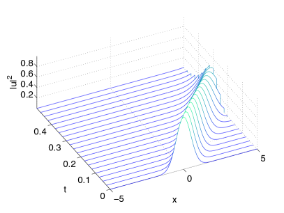
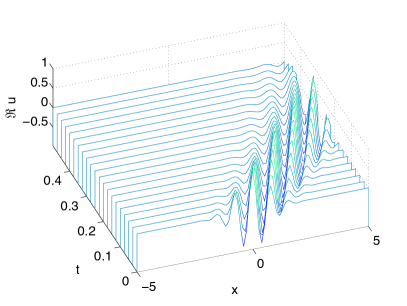
Figure 1. Exact solution (50) to the free Schrödinger equation being used as a test of the various numerical approaches; on the left the modulus squared of the solution, on the right its real part.

The solution (50) can be constructed from the well known solution to the Schrödinger equation for Gaussian initial data by exploiting the Galilei invariance of the Schrödinger equations of the form (1). This means, that if $u(t,x)$ is a solution, then so is

(51) $$\hat{u}(x,t)=u(x-ct,t)e^{icx/2-ic^{2}t/4},$$

with $c\in\mathbb{R}$ some finite speed.

Remark 6.1.

It is convenient in practical computations for data with a single maximum to exploit the Galilean invariance of the equation by going to a reference frame essentially travelling with the maximum. In this way, it is straight forward to choose an optimal resolution for different domains in CED approaches. This can be even done by going to an accelerated frame and thus changing the form of the to be solved equation as for instance in [20]. For the example (50), this would imply the study of the dispersed Gaussian with a maximum fixed at the origin. Since the solution is rapidly decreasing, Fourier techniques would certainly be most efficient here. However, the goal of the present paper is to compare the efficiency of various numerical approaches in dealing with a maximum passing through the domain boundary which is why we do not switch to a moving frame here and use the example of [36].

For the CED method, we choose $N^{I}=20$, $N^{II}=120$ and $N^{III}=600$ Chebyshev points in the respective domains. It can be seen in Fig. 2 that the Chebyshev coefficients (5) decrease in each of the domains to machine precision, both for the initial and the final time of the computation. Note that the Chebyshev coefficients in domain I are always completely of the order of machine precision (they are covered in the left figure in Fig. 2 by the coefficients in domain III) which means one could just impose vanishing Dirichlet condition at $x_{l}$. The domain is mainly kept here to illustrate the approach.

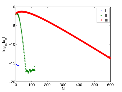
Figure 2. Chebyshev coefficients (5) for the solution (50) in the three domains; on the left at $t=0$, on the right for $t=0.5$.

As in [36], we will discuss in the following the numerical error $\Delta$ as the $L^{2}$ norm of the difference between numerical solution $u$ and exact solution $u_{ex}$ normalized by the $L^{2}$ norm of the exact solution,

(52) $$\Delta=\frac{||u-u_{ex}||_{2}}{||u_{ex}||_{2}}.$$

For PML and TBC, both are computed for $x\in[x_{l},x_{r}]$, for CED for $x\in\mathbb{R}$. This is done with the Clenshaw-Curtis algorithm outlined in section 2.

We first compare the various approaches with second order CN method in all cases. The numerical error $\Delta$ for the CED method can be seen in Fig. 3 on the left. Because of the matching conditions at the domain boundaries, this is a global method on the whole real line, and no effect should be visible in this approach when the maximum crosses the boundary at $t=0.3125$. It can be seen that this is indeed the case, the numerical error increases in time due to a piling up of the errors in the time integration. In Fig. 3, the numerical error is shown for three resolutions ($N_{t}=10^{3},10^{4},10^{5}$). It can be clearly seen that the CN method shows the expected second order behavior. A precision of the order of $10^{-7}$ can be reached in this example, for higher accuracies a fourth order method as discussed below would be clearly the better choice.

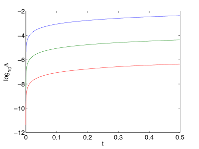
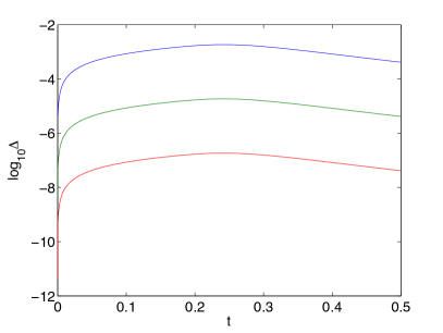
Figure 3. Normalized $L^{2}$ norm $\Delta$ of the difference between numerical and exact solution (52) with CN method for $N_{t}=10^{3}$, $N_{t}=10^{4}$ and $N_{t}=10^{5}$ time steps (from top to bottom); on the left for the CED method the error on the whole line, on the right for the TBC method in the computational domain.

In Fig. 3, the same situation is studied on the right for the TBC approach. Here we only have domain II where we use the same resolution as before ($N^{II}=120$). Since both CED and TBC can be treated explicitly, the latter is considerably more efficient since only one domain is considered. The numerical error behaves slightly differently in this case as can be recognized in Fig. 3: once considerable parts of the mass of the solution leave around $t\approx 0.3$ the domain, the numerical error there decreases slightly since the solution itself is almost zero in part of the domain. There are no spurious reflections at the boundary if sufficient resolution in time is provided, the conditions are really transparent within numerical precision which is theoretically expected, see [1]. The CN scheme again shows the expected second order behavior.

As can be seen in Fig. 4 on the left, the numerical error in the PML case with CN is very similar to the TBC case. Again second order convergence of the time integration scheme is observed, and the numerical error (52) decreases once most of the mass leaves the computational domain. We use here $N^{I}=20$ and $N^{III}=50$ Chebyshev collocation points and find that the Chebyshev coefficients (5) decrease to $10^{-12}$ in the layers throughout the computation. This shows that much less spatial resolution is needed here in domain III compared to the CED approach. Thus for the shown accuracy range, the PML method is less efficient than TBC, but more so than CED.

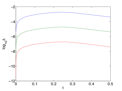
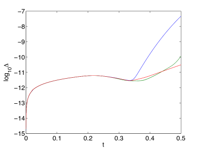
Figure 4. On the left, normalized $L^{2}$ norm $\Delta$ of the difference between numerical and exact solution (52) with CN method for $N_{t}=10^{3}$, $N_{t}=10^{4}$ and $N_{t}=10^{5}$ time steps (from top to bottom) for the PML method with $\sigma_{0}=50$ and $\delta=0.5$; on the right the PML approach with IRK4 method and $N_{t}=10^{4}$ for various values of $\sigma_{0}$ in (22) ($\sigma_{0}=40,50,60$ corresponding to the blue, green, and red curve respectively).

The above examples with the second order scheme CN in Fig. 3 and 4 show that it is hardly possible to reach machine precision with such an approach. Therefore we apply the fourth order IRK4 method here to illustrate the difference. It is an advantage of both PML and CED that it is straight forward to combine them with convenient time integration schemes. It can be seen in Fig. 5 that essentially the same accuracy can be reached for $N_{t}=10^{3}$ as with $10^{5}$ time steps for CN in Fig. 3, and that with $N_{t}=10^{4}$ one essentially reaches machine precision for the CED method.

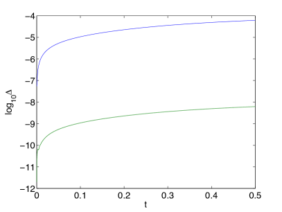
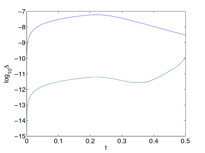
Figure 5. Normalized $L^{2}$ norm $\Delta$ of the difference between numerical and exact solution (52) with IRK4 method for $N_{t}=10^{3}$ and $N_{t}=10^{4}$ time steps (from top to bottom); on the left for the CED method the error on the whole line, on the right for the PML method with $\delta=0.5$ and $\sigma_{0}=50$ in the computational domain.

For the PML method, the same situation is shown on the right of Fig. 5. The behavior for $N_{t}=10^{3}$ is as expected from the CED case and the CN approach for PML in Fig. 4. But for the even higher resolution $N_{t}=10^{4}$, an effect of the right layer can be seen. After the maximum of the solution hits the domain boundary at $t=0.3125$, the numerical error increases again in the computational domain due to reflections from the layer. This is why the values for $\delta$ and $\sigma_{0}$ in (22) were fixed after studying the numerical error with the IRK4 method in Fig. 4 on the right. Since both $\delta$ and $\sigma_{0}$ have the same effect to increase the effective length $|\tilde{x}|$ of the layer where the dissipation is active, we fix as in [36] $\delta=0.5$ and vary $\sigma_{0}$ to minimize the numerical error. It can be seen in Fig. 4 that the numerical error $\Delta$ increases strongly for $\sigma_{0}=40$ once the maximum of the solution enters the layer. This is much less the case for larger $\sigma_{0}$, but $\sigma_{0}=60$ produces a larger error near $t=0.3125$ than $\sigma_{0}=50$. Since it is most important to resolve the solution well in the computational domain whilst there is still considerable mass there, we chose $\sigma_{0}=50$ for the computations. The need to optimize the value of $\sigma_{0}$ essentially by trial and error, i.e., by additional runs of the code for the same initial data, is a clear disadvantage of the PML approach. Note however that in the present example, there is no visible effect by choosing either of these three values for $\sigma_{0}$ with the CN method on the left of Fig. 4 since the accuracy of the time integration scheme is too low.

Note also that the error shown for CED is obtained on the whole axis whereas it is for PML only for the computational domain. Thus it is not surprising that the error is smaller for PML at later times since the solution is close to zero after a certain time in the computational domain, whereas the maximum of the solutions is being tracked outside this domain in the CED approach.

7. Numerical study of the NLS soliton

In this section we study the CED, TBC and PML approaches for the NLS equation at the example of the NLS soliton,

(53) $$u(x,t)=\sqrt{a}\mbox{ sech}\sqrt{a}(x-ct)\exp\left[i\left(\frac{c}{2}x+\left(a-\frac{c^{2}}{4}\right)t\right)\right]$$

for $a=2$ and $c=15$ and $t\leq 2$ shown in Fig. 6. The exact solution (53) is imposed as initial condition at $t=0$, and the numerical error $\Delta$ is defined as in (52). We use $x_{r}=-x_{l}=25$ to assure that the solution is almost of the order of machine precision at the boundaries (here $\sim 10^{-11}$). This is important since both the TBC and the PML approach in the form used here assume initial data with compact support (at least within numerical precision) in the domain $[x_{l},x_{r}]$. As in [36], the PML approach for NLS does not dissipate the solution well in the layer which leads to errors in the computational zone.

As can be seen in Fig. 6, the localized solution travels with constant speed $c=15$ to the right. Its maximum hits the boundary of domain II at $t=1.666\ldots$. The real part in the same figure shows the oscillatory phase of the solution that is stationary in a comoving frame (obtained by applying (51)). In such a frame, Fourier methods with time integrators as in [18] would be the ideal choice, but as in the previous section, the goal is here to study the efficiency of the respective method when the soliton crosses the boundary.

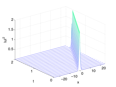
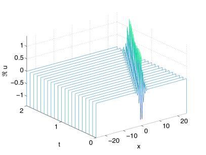
Figure 6. Soliton solution (53) to the cubic NLS equation being used as a test for the various numerical approaches; on the left the modulus squared of the solution, on the right its real part.

We again study the spatial resolution for the CED method and choose $N^{I}=20$, $N^{II}=700$ and $N^{III}=500$ Chebyshev points in the respective domains. It can be seen in Fig. 7 that the Chebyshev coefficients (5) decrease in each of the domains at least to $10^{-12}$ for this choice, both for the initial and the final time of the computation. Note that the Chebyshev coefficients in domain I are again completely of the order of machine precision which means one could just impose vanishing Dirichlet condition at $x_{l}$.

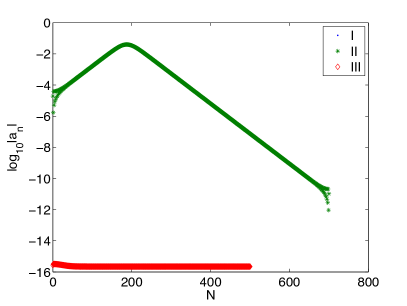
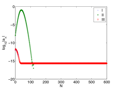
Figure 7. Chebyshev coefficients (5) for the solution (53) in the three domains; on the left at $t=0$, on the right for $t=2$.

As in the previous section, we first compare the various methods with the second order CN scheme in all cases. The numerical error $\Delta$ for the CED method can be seen in Fig. 8 on the left. The global character of the approach ensures once more that no effect is visible in the error when the maximum crosses the boundary at $t=1.666\ldots$. Since all approaches are now iterative due to the nonlinearity of the NLS equation in contrast to the linear case of the previous section, we only consider the resolutions $N_{t}=10^{3}$ and $N_{t}=10^{4}$. It can be clearly seen that the CN method shows the expected second order behavior. A precision of the order of $10^{-3}$ can be reached in this example without problems, for higher accuracies a fourth order method as discussed below would be clearly the better choice.

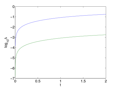
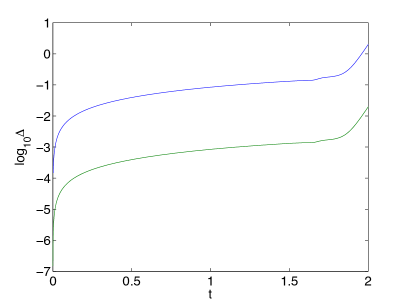
Figure 8. Normalized $L^{2}$ norm $\Delta$ (52) of the difference between numerical and exact solution with CN method for $N_{t}=10^{3}$ and $N_{t}=10^{4}$ time steps (from top to bottom); on the left for the CED method the error on the whole line, on the right for the TBC method in the computational domain.

In Fig. 8, the same situation is studied on the right for the TBC approach. There is only domain II in this case where we use the same resolution as for CED ($N^{II}=700$). Due to the much lower overall spatial resolution needed than in the CED case, the method is slightly more efficient. But this is partly offset by the need to iterate the Dirichlet to von Neumann map. Whereas this has little effect for $x=x_{l}$ since the solution vanishes with numerical precision there, the iteration takes more and more time once the maximum of the solution approaches the boundary $x=x_{r}$. In addition the numerical error normalized by the $L^{2}$ norm of the exact solution within the computational domain now increases strongly once the maximum of the solution passes the boundary. For $N_{t}=10^{3}$ it is even of order 1, for $N_{t}=10^{4}$ of the order of $1\%$. The error normalized by the $L^{2}$ norm of the initial data still decreases to the order of $10^{-3}$ and $10^{-5}$ respectively. But the increase of the error in Fig. 8 is in clear contrast to the linear case in Fig. 3 where the error even decreases. The reason for this appears to be that the Dirichlet to von Neumann map has to be obtained also approximatively, whereas it is explicitly known in the linear case. The CN scheme though shows the expected second order behavior in both cases, it is just computationally expensive to reach higher precision with a second order scheme.

As can be seen in Fig. 9 on the left, the numerical error in the PML case with CN is obviously different from the TBC case. Again second order convergence of the time integration scheme is observed whilst most of the mass is within the computational domain, but the numerical error (52) increases once most of the mass leaves the latter, and this even in a way independent of the time resolution at a given point. We use here $N^{I}=50$ and $N^{III}=100$ Chebyshev collocation points to assure that the Chebyshev coefficients (5) decrease to machine precision throughout the computation in the layers. Again a much lower values of $N^{III}$ is needed here compared to the CED approach.

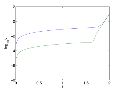
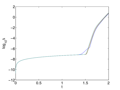
Figure 9. On the left, normalized $L^{2}$ norm $\Delta$ of the difference between numerical and exact solution (52) with CN method for $N_{t}=10^{3}$ and $N_{t}=10^{4}$ time steps (from top to bottom) for the PML method with $\sigma_{0}=3$ and $\delta=1$; on the right the PML approach with IRK4 method and $N_{t}=5000$ for various values of $\sigma_{0}$ in (22) ($\sigma_{0}=2,3,5,10$ corresponding to the blue, green, red and cyan curve respectively).

To reach higher precision we apply again the fourth order IRK4 method which can be implemented for both PML and CED in a straight forward way. The fourth order convergence can be seen in Fig. 10. For CED, with $N_{t}=10^{4}$ one is already close to machine precision.

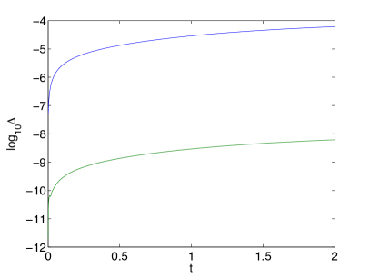
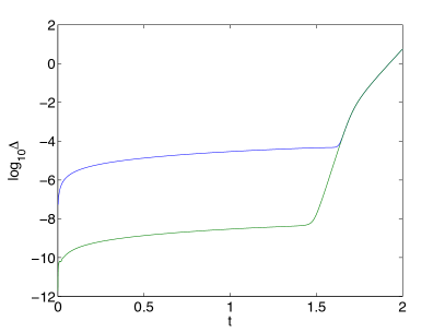
Figure 10. Normalized $L^{2}$ norm $\Delta$ of the difference between numerical and exact solution (52) with IRK4 method for $N_{t}=10^{3}$ and $N_{t}=10^{4}$ time steps (from top to bottom); on the left for the CED method the error on the whole line, on the right for the PML method with $\delta=1$ and $\sigma_{0}=3$ in the computational domain.

For the PML method, the same situation is shown on the right of Fig. 10. As with the CN method in Fig. 9, the expected convergence of the scheme is only observed whilst most of the mass of the solution is within the computational domain. Once the maximum of the solution is close to the boundary, the error becomes independent both of the spatial and the temporal resolution and is thus clearly an effect of the PML approach. As observed already in [36], the layers are clearly not ‘perfectly matched’ in the nonlinear case. This also does not change if we vary the parameter $\sigma_{0}$ in the right figure of Fig. 9. There we put $\delta=1$ and vary $\sigma_{0}$ to minimize the numerical error. It can be seen in Fig. 9 that the numerical error $\Delta$ is almost identical for the values $2,3,5,10$, but that it is worst for the values 2 and 10 in this example. Thus we choose $\sigma_{0}=3$ since it also performs best close to the time when the maximum of the solution reaches the boundary of the computational domain.

To illustrate the behavior of the numerical solution for TBC and PML near the boundary, we show in Fig. 11 the difference of the numerical and exact solutions in both cases at $t=2$ for CN with $N_{t}=10^{4}$. It can be seen that the absolute error for TBC is of the order $10^{-5}$ and that some spurious reflections propagate to the left. These might be further reduced if a higher resolution in time is used. The absolute error for PML on the other hand is of the order of $1\%$, and the solution in the computational domain is clearly affected near the boundary. This effect cannot be reduced if the resolution in time or space is increased, nor if different values of $\sigma_{0}$ are used.

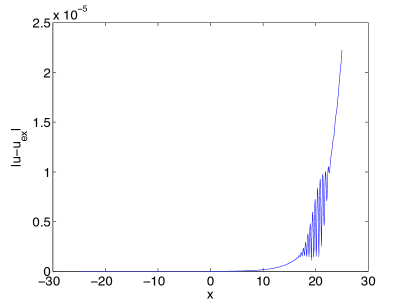
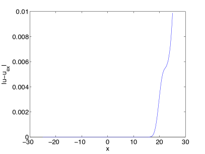
Figure 11. Difference between numerical and exact solution to NLS for soliton initial data (53) for the TBC method on the left and for the PML method on the right at $t=2$ for $N_{t}=10^{4}$ with the CN method.

8. Numerical study of the Peregrine breather

The TBC and the PML method used in this article are constructed for initial data with compact support in the computational domain, a condition which should be satisfied with the aimed at precision. CED methods on the contrary just require fall off to some (possibly nonzero) constant (for fixed $t$) at infinity which may be slow. To illustrate this we consider the celebrated Peregrine breather solution to the NLS equation which is discussed as a possible candidate for rogue waves in hydrodynamics and nonlinear optics. The solution can be seen in Fig. 12.

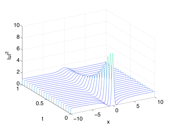
Figure 12. Peregrine breather (2).

For $|x|\to\infty$, one has that $|u|\to 1$. The solution is also slowly dispersed away for $t\to\infty$. We show in this section that the breather solution can be numerically evolved on the whole real line with essentially machine precision. This allows to study numerically the stability of the breather solution. This is important in the context of rogue waves since experimentally observable structures should be stable to a certain extent. A stability analysis for periodic breathers was presented in [11], an experimental study of the stability of the Peregrine breather appearing in hydrodynamical experiments against wind was described in [10].

We give the Peregrine solution for $t=0$ as initial data and numerically solve NLS with these data for $t\leq 1$. To this end we choose $x_{r}=-x_{l}=10$, $N^{I}=N^{III}=50$ and $N^{II}=700$. It can be seen in Fig.13 that the Chebyshev coefficients (5) decrease to machine precision in this case during the whole computation.

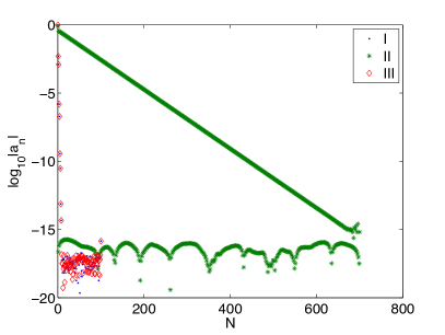
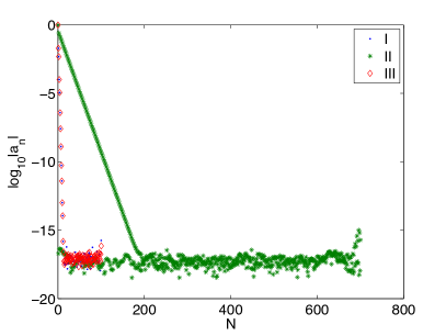
Figure 13. Chebyshev coefficients (5) for the solution (2) in the three domains; on the left at $t=0$, on the right for $t=1$.

Note that we get essentially the same numerical result with the more symmetric (in the $N^{i}$) choice $x_{r}=-x_{l}=5$ and $N^{I}=N^{III}=200$, $N^{II}=400$. We use here only the IRK4 method since we are interested in testing with which accuracy the solution can be reproduced. Since the Peregrine solution is not in $L^{2}(\mathbb{R})$, we consider here the numerical error defined via the $L^{\infty}$ norm,

(54) $$\Delta_{\infty}=\frac{||u-u_{Per}||_{\infty}}{||u_{Per}||_{\infty}},$$

where $u_{Per}$ is the solution (2). It can be seen in Fig. 14 that the numerical error is smaller than $10^{-10}$ for $N_{t}=1000$, and that one is close to the optimum with $N_{t}=2000$.

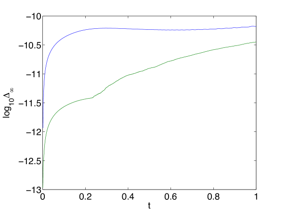
Figure 14. $L^{\infty}$ norm $\Delta_{\infty}$ (54) of the difference between numerical and exact solution to NLS for Peregrine initial data (2) for the CED approach with IRK4 method with $N_{t}=1000$ and $N_{t}=2000$ (from top to bottom).

If no exact solution is known for given initial data, it is convenient to use conserved quantities of the studied PDE, whose conservation is not implemented in the code, to control the accuracy of the numerical solution, see for instance the discussion in [18]. Since the cubic NLS equation is completely integrable, there is an infinite number of conserved quantities, the most popular being the mass (the $L^{2}$ norm of the solution) and the energy. Note that both these quantities are not defined for the breather since it is not in $L^{2}$, but that the combination

(55) $$E=\frac{1}{2}\int_{\mathbb{R}}\left\{|u_{x}|^{2}-|u|^{2}(|u^{2}|-1)\right\}dx$$

is both conserved and defined. It can be checked by direct computation that $E=0$ for the Peregrine breather. For given $u$, the integral in (55) will be computed as discussed in section 2 with the Clenshaw-Curtis algorithm after division by $s_{l}$ and $s_{r}$ in coefficient space in the compactified domains. In numerical simulations, the quantity $E$ will depend on time due to unavoidable numerical errors. We use the relative quantity $\Delta_{E}=|1-E(t)/E(0)|$ as an indicator of the accuracy of the solution. As discussed in [18], such quantities are reliable indicators of the precision if sufficient resolution in $x$ is provided, but tend to overestimate the accuracy by one to two orders of magnitude. For the exact Peregrine solution, the quantity $E$ is numerically of the order of $10^{-13}$, i.e., machine precision.

Since the CED approach allows to propagate Peregrine initial data essentially with machine precision, we are able to study localized perturbations of the breather: as an example we consider initial data $u_{Per}(x,0)+0.1\exp(-x^{2})$, i.e., the Peregrine solution at time $t=0$ perturbed by a small Gaussian. We use $N^{I}=N^{II}=N^{III}=400$ and $N_{t}=1000$ for the computation. It can be seen in Fig. 15 that the solution appears to be dispersed away to infinity, but in a significantly different way than the Peregrine breather. This is even more obvious in the right figure of Fig. 15 where the solution at the last computed time is shown with the Peregrine solution (2) at the same time.

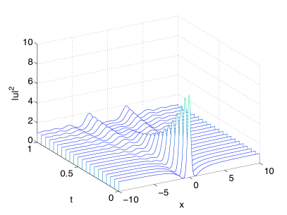
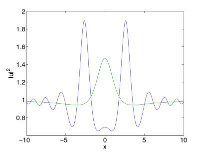
Figure 15. Solution to the NLS equation for the initial data $u_{Per}(x,0)+0.1\exp(-x^{2})$ in dependence of time on the left; on the right the solution at the final time in blue and the Peregrine solution at the same time in green.

Thus it appears that the Peregrine breather is unstable against this type of perturbations, and that the perturbed solution does not stay close to the exact solution. Note that the solution is even at the last computed time well resolved spatially as can be seen in the right figure of Fig. 16, where the Chebyshev coefficients (5) at the last computed time are shown. Since the initial data is symmetric with respect to the transformation $x\to-x$ and since the Schrödinger equation preserves parity, the Chebyshev coefficients in zone I and III are identical, and half of the coefficients in zone II vanish with numerical precision. The coefficients in zone I and III still decrease to $10^{-4}$ which indicates that the solution is computed to better than plotting accuracy. The slow decrease of the Chebyshev coefficients is due to the oscillations shown on the left of Fig. 16. The relative conserved energy $\Delta_{E}\sim 8.8*10^{-3}$. This implies together with the resolution in coefficient space shown in Fig. 16 that the solution is computed to at least plotting accuracy.

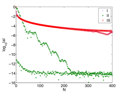
Figure 16. Solution to the NLS equation at $t=1$ for the initial data $u_{Per}(x,0)+0.1\exp(-x^{2})$ in the compactified domain on the left, and the corresponding Chebyshev coefficients (5) on the right.

9. Outlook

In this paper we have presented a multidomain spectral method with compactified exterior domains for Schrödinger equations and discussed examples for the linear Schrödinger and cubic NLS equations. The solutions have to be bounded at spatial infinity. The method was compared to exact TBC and PML approaches. It was shown that it produces results of at least the same quality as TBC and PML in the linear case, and that machine precision can be reached with a fourth order time integrator. The price to pay for this is that the solution has to be resolved with the wanted precision on the whole real line. Thus if one is only interested in the solution in the computational domain, TBC and PML approaches might be more economic, though the latter approach in practice requires several runs to optimize the parameters. The slight disadvantage of CED disappears, however, in the nonlinear case where even TBC methods need an approximate (and iterative) solution of the Dirichlet to von Neumann map, and where the PML method [36] produces considerable errors. In contrast, the CED method could reach the same precision as in the linear case and seems therefore the preferred choice for high precision studies.

The real advantage of the CED method is, however, for situations with an algebraic fall off towards infinity whereas TBC and PML require initial data with compact support. As an example we studied the Peregrine breather (2) which is discussed as a model for rogue waves in hydrodynamics and nonlinear optics. As was shown, the CED approach can propagate this solution with machine precision and allows the study of perturbations which will be done in more detail elsewhere. The approach is also open to a generalization to higher dimensions where soliton solutions often have an algebraic fall off, see the lump of Davey-Stewartson and Kadomtsev-Petviashvili equations ($2+1$ dimensional generalizations of NLS and Korteweg-de Vries equations respectively). This will be the subject of further research.

References

- [1] X. Antoine, A. Arnold, C. Besse, M. Ehrhardt, A. Schädle. A Review of Transparent and Artificial Boundary Conditions Techniques for Linear and Nonlinear Schrödinger Equations. Comm. Comput. Phys. 4, 729-796 (2008).
- [2] X. Antoine and C. Besse. Unconditionally stable discretization schemes of non-reflecting boundary conditions for the one-dimensional Schrödinger equation. J. Comput. Phys., 188(1), 157-175 (2003).
- [3] H. Bailung, S. K. Sharma, and Y. Nakamura, Observation of Peregrine solitons in a multicomponent plasma with negative ions, Phys. Rev. Lett. 107, 255005 (2011).
- [4] V.A. Baskakov and A.V. Popov. Implementation of transparent boundaries for numerical solution of the Schrödinger equation. Wave Motion, 14(2), 123-128 (1991).
- [5] J. Bérenger. A perfectly matched layer for the absorption of electromagnetic waves. J. Comput. Phys. 114, 185-200, 1994.
- [6] A. Boutet de Monvel, A.S. Fokas and D. Shepelsky, Analysis of the global relation for the nonlinear Schrödinger equation on the half-line, Lett. Math. Phys. 65, 199-212 (2003).
- [7] L. Burgnies, O. Vanbésien and D. Lippens, Transient analysis of ballistic transport in stublike quantum waveguides, Appl. Phys. Lett. 71, 803-805 (1997).
- [8] A. Chabchoub, N. P. Hoffmann, and N. Akhmediev, Rogue wave observation in a water wave tank, Phys. Rev. Lett. 106, 204502 (2011).
- [9] A. Chabchoub, N. Hoffmann, M. Onorato, and N. Akhmediev, Super rogue waves: observation of a higher-order breather in water waves, Phys. Rev. X 2, 011015 (2012).
- [10] A. Chabchoub, N. Hoffmann, H. Branger, C. Kharif, and N. Akhmediev, Experiments on wind-perturbed rogue wave hydrodynamics using the Peregrine breather model, Physics of Fluids 25 (2013) DOI: 10.1063/1.4824706
- [11] A. Calini and C. M. Schober, Nat. Hazards Earth Syst. Sci., 14, 1431-1440 (2014).
- [12] J.F. Claerbout, Coarse grid calculation of waves in inhomogeneous media with application to delineation of complicated seismic structure, Geophysics 35, 407-418 (1970).
- [13] P. Dubard, P. Gaillard, C. Klein and V.B. Matveev, On multi-rogue wave solutions of the NLS equation and positon solutions of the KdV equation, Eur. Phys. J. Special Topics 185, 247-258 (2010)
- [14] J. Duque, Solving time-dependent equations of Schrödinger-type using mapped infinite elements, Int. J. Mod. Phys. C 16, No. 2 309-316 (2005).
- [15] T. Hagstrom, Radiation boundary conditions for the numerical simulation of waves, Acta Numerica 8, 47-106 (1999).
- [16] S. G. Johnson. Notes on Perfectly Matched Layers (PMLs) (2010), http://math.mit.edu/ stevenj/18.369/pml.pdf.
- [17] B. Kibler, J. Fatome, C. Finot, G. Millot, F. Dias, G. Genty, N. Akhmediev, and J. M. Dudley, The Peregrine soliton in nonlinear fibre optics, Nat. Phys. 6, 790-795 (2010).
- [18] C. Klein, Fourth order time-stepping for low dispersion Korteweg-de Vries and nonlinear Schrödinger equation, ETNA Vol. 29 116-135 (2008).
- [19] C. Klein and K. Roidot, Fourth order time-stepping for Kadomtsev-Petviashvili and Davey-Stewartson equations, SIAM J. Sci. Comput., 33(6), 3333-3356. DOI: 10.1137/100816663 (2011).
- [20] C. Klein and R. Peter, Numerical study of blow-up in solutions to generalized Korteweg-de Vries equations, arXiv:1307.0603
- [21] X. Antoine, C. Besse, and P. Klein. Absorbing Boundary Conditions for the One-Dimensional Schrödinger Equation with an Exterior Repulsive Potential, Journal of Computational Physics, 228(2), 312-335 (2009).
- [22] F. Ladouceur, Boundaryless beam propagation, Opt. Lett. 21, 4-5 (1996).
- [23] C. Lanczos, Trigonometric interpolation of empirical and analytic functions, J. Math. and Physics, 17, 123-199 (1938)
- [24] M.F. Levy, Parabolic equation models for electromagnetic wave propagation, IEE Electromagnetic Waves Series 45 (2000).
- [25] C.W. McCurdy, D.A. Homer and T.N. Resigno, Time dependent approach to collisional ionization using exterior complex scaling, Phys. Rev. A 65, 042714 (2002).
- [26] A. Nissen, G. Kreiss. An Optimized Perfectly Matched Layer for the Schrödinger Equation. Rapport technique, Department of Information Technology, Uppsala University (2009).
- [27] C.E. Grosch and S.A. Orszag, Numerical solution of problems in unbounded regions: coordinate transforms, J. Comput. Phys. 25, 273-296 (1977).
- [28] D.H. Peregrine, Water waves, nonlinear Schrödinger equations and their solutions, J. Austral. Math. Soc. B 25 16-43 (1983), doi:10.1017/S0334270000003891
- [29] F. Schmidt and P. Deuflhard, Discrete transparent boundary conditions for the numerical solution of FresnelÕs equation, Comput. Math. Appl. 29, 53-76 (1995).
- [30] F.D. Tappert, The parabolic approximation method, in Wave Propagation and Underwater Acoustics, Lecture Notes in Physics 70, eds. J.B. Keller and J.S. Papadakis, Springer, New York, 224-287 (1977).
- [31] S.V. Tsynkov. Numerical solution of problems on unbounded domains. A review. Appl. Numer. Math., 27(4), 465-532 (1998).
- [32] L.N. Trefethen, Spectral Methods in Matlab. SIAM, Philadelphia, PA (2000)
- [33] www.comlab.ox.ac.uk/oucl/work/nick.trefethen
- [34] www.lorene.obspm.fr
- [35] V.E. Zakharov and A.B. Shabat, Exact theory of two-dimensional self-focusing and one-dimensional self- modulation of waves in nonlinear media. Sov. Phys. JETP 34(1), 62-69 (1972); translated from Zh. Eksp. Teor. Fiz. 1, 118-134 (1971)
- [36] C. Zheng. A perfectly matched layer approach to the nonlinear Schrödinger wave equations. J. Comput. Phys. 227, 537-556 (2007).
- [37] C. Zheng, Exact nonreflecting boundary conditions for one-dimensional cubic nonlinear Schrödinger equations, J. Comput. Phys. 215, 552-565 (2006).