Dynamics and thermodynamics of a pair of interacting magnetic dipoles

Abstract

We consider the dynamics and thermodynamics of a pair of magnetic dipoles interacting via their magnetic fields. We consider only the “spin" degrees of freedom; the dipoles are fixed in space. With this restriction it is possible to provide the general solution of the equations of motion in analytical form. Thermodynamic quantities, such as the specific heat and the zero field susceptibility are calculated by combining low temperature asymptotic series and a complete high temperature expansion. The thermal expectation value of the autocorrelation function is determined for the low temperature regime including terms linear in $T$. Furthermore, we compare our analytical results with numerical calculations based on Monte Carlo simulations.

I Introduction

Systems in which magnetic nanostructures solely interact via electromagnetic forces have recently drawn much attention experimentally as well as theoretically EW13 - JO98 . Whereas in traditional magnetic systems electromagnetic forces usually just add to a complex exchange interaction scenario, they play a major role in arrays of interacting magnetic nanoparticles and lithographically produced nanostructures. In such systems geometrical frustration and disorder lead to interesting and exotic low temperature effects, e. g. artificial spin ice W06 , C08 , and superspin glass behavior H11 . Moreover, these systems are promising candidates for future applications beyond magnetic data-storage, e. g. , as low-power logical devices I06 , E14 . Theoretically, these systems can often be described as interacting point dipoles. This is justified if the considered nanostructures form single domain magnets and are spatially well separated from each other so that exchange interactions do not play an important role. In this paper, we show that the dynamical and thermodynamical properties of the basic building block of such systems, a pair of interacting point dipoles, can rigorously be treated analytically by combining low temperature asymptotic series and a complete high temperature expansion. A considerable part of these calculations has been performed with the aid of the computer algebra system MATHEMATICA 9.0.

From a mathematical point of view, the system of two interacting magnetic dipoles is equivalent to a classical spin system with $N=2$ and the particular XXZ Hamiltonian (13). Hence our results can be applied to these systems as well.

The paper is organized as follows. For the reader’s convenience we recapitulate in section II.1 the derivation of the equation of motion (eqm) of two interacting dipoles and identify the underlying assumptions. The solution of the eqm in terms of elliptic integrals and the Weierstrass elliptic function in section II.2 is based on the existence of two conserved quantities. The limiting case of solutions close to the ground state can be described by harmonic oscillations with three frequencies, see section II.3. In the next sections we discuss the thermodynamics of the dipole pair. After explaining our methods we calculate the partition function (section III.2), the specific heat (section III.3) and the zero field susceptibility (section III.4) by combining low- and high-temperature expansions. The latter two physical properties are also determined by Monte Carlo simulations and shown to closely coincide with the theoretical results. Since the problem is anisotropic we have to distinguish between different susceptibilities w. r. t. the “easy axis", the axis joining the two dipoles, and the “hard axis", any axis perpendicular to the easy axis. For the easy axis susceptibility there occur complications for the standard Monte Carlo simulations that have been overcome by using the so-called Exchange Monte Carlo method, see H96 . Similarly the autocorrelation function is calculated in the low temperature limit and compared with simulation results at low temperatures, see section III.5. We find that one of the three frequencies mentioned above is suppressed by thermodynamical averaging. Appendix A contains a short introduction into the theory of elliptic integrals and elliptic functions for those readers who are not acquainted with this subject. The Appendices B – D contain details of the theoretical derivations presented in the main part of the paper. We close with a summary and outlook.

II Dynamics

II.1 Derivation of the equation of motion

We consider two identical magnetic dipoles, labeled by an index $i=1,2$, that are fixed in space and separated by a distance $a$. We denote the magnetic moment vector of dipole $i$ by ${\mathbf{m}}_{i}$ and assume that it is associated with an angular momentum ${\mathbf{L}}_{i}$ according to the standard formula

$${\mathbf{m}}_{i}=\gamma\;{\mathbf{L}}_{i}\;,\quad i=1,2\;,$$ (1)

where $\gamma$ is the gyromagnetic ratio

$$\gamma=-\frac{e_{0}}{2m_{e}}g\;,$$ (2)

independent of $i$. $\gamma$ is assumed to be negative due to the negative charge $-e_{0}$ of the electron ($m_{e}$ denoting its mass) and the gyromagnetic factor $g$ is considered as a physical property of the dipoles. We expect that $g$ varies between $g=1$ for the contribution due to pure orbital motion of the electrons and $g=2$ for the spin contribution to the magnetism of the dipoles. Furthermore we will assume that the torque exerted on a dipole by a magnetic field ${\mathbf{B}}$ is equal to

$${\mathbf{N}}={\mathbf{m}}\times{\mathbf{B}}\;.$$ (3)

This textbook equation is usually derived for systems of moving charges and constant magnetic fields. Hence the validity of (3) for the problem under consideration is not trivial but an additional assumption. In our case there are two magnetic fields, ${\mathbf{B}}_{1}$ and ${\mathbf{B}}_{2}$, where ${\mathbf{B}}_{2}$ denotes the instantaneous value of the magnetic field at ${\mathbf{m}}_{1}$ due to dipole $2$, and an analogous definition applies for ${\mathbf{B}}_{1}$ due to dipole $1$. Thus, for example,

$${\mathbf{B}}_{2}=\frac{\mu_{0}}{4\pi a^{3}}\left(3{\mathbf{m}}_{2}\cdot{\mathbf{e}}\;{\mathbf{e}}-{\mathbf{m}}_{2}\right)\;,$$ (4)

where ${\mathbf{e}}$ is a unit vector parallel to the constant position vector from dipole $1$ to dipole $2$. Hence we obtain

$$\frac{d}{dt}{\mathbf{m}}_{1} = \gamma\;\frac{d}{dt}{\mathbf{L}}_{1}=\gamma{\mathbf{m}}_{1}\times{\mathbf{B}}_{2}$$ (5)

$$= \frac{\gamma\mu_{0}}{4\pi a^{3}}{\mathbf{m}}_{1}\times\left(3{\mathbf{m}}_{2}\cdot{\mathbf{e}}\;{\mathbf{e}}-{\mathbf{m}}_{2}\right)\;.$$

Introducing the unit vectors ${\mathbf{s}}_{i}=\frac{1}{M}{\mathbf{m}}_{i},\;i=1,2$ where $M=|{\mathbf{m}}_{1}|=|{\mathbf{m}}_{2}|$ is constant, and utilizing (2) we rewrite (5) as

$$\frac{d}{dt}{\mathbf{s}}_{1} = -\frac{\mu_{0}e_{0}\,g\,M}{8\,\pi\,m_{e}\,a^{3}}\;{\mathbf{s}}_{1}\times\left(3{\mathbf{s}}_{2}\cdot{\mathbf{e}}\;{\mathbf{e}}-{\mathbf{s}}_{2}\right)$$ (6)

$$= -\omega_{0}\;{\mathbf{s}}_{1}\times\left(3{\mathbf{s}}_{2}\cdot{\mathbf{e}}\;{\mathbf{e}}-{\mathbf{s}}_{2}\right)\;.$$ (7)

Here we have introduced the constant $\omega_{0}$, with dimension 1/time, defined by

$$\omega_{0}\equiv\frac{\mu_{0}e_{0}\,g\,M}{8\,\pi\,m_{e}\,a^{3}}\;.$$ (8)

Using $\omega_{0}t$ as a dimensionless time variable, again denoted by $t$, and considering the analogous equation of motion (eqm) for the second dipole, we eventually obtain the following system of coupled first order differential equations:

$$\frac{d}{dt}{\mathbf{s}}_{1} = -{\mathbf{s}}_{1}\times\left(3{\mathbf{s}}_{2}\cdot{\mathbf{e}}\;{\mathbf{e}}-{\mathbf{s}}_{2}\right)\;,$$ (9)

$$\frac{d}{dt}{\mathbf{s}}_{2} = -{\mathbf{s}}_{2}\times\left(3{\mathbf{s}}_{1}\cdot{\mathbf{e}}\;{\mathbf{e}}-{\mathbf{s}}_{1}\right)\;.$$ (10)

In view of possible applications mentioned in the Introduction we stress that the derivation of the eqm (9), (10) is based on the following two idealized assumptions:

• The two dipoles can be assumed as point-like objects, and

• the constant $\omega_{0}$ is small enough such that the quasi-static approximation of the complete set of Maxwell’s equations is valid.

II.2 Solution of the equation of motion

To facilitate solving the eqm (9), (10) we first note that these equations give rise to two conserved physical quantities, to be denoted by $Q_{1}$ and $Q_{2}$:

$$Q_{1}={\mathbf{S}}\cdot{\mathbf{e}}\;,$$ (11)

where ${\mathbf{S}}\equiv{\mathbf{s}}_{1}+{\mathbf{s}}_{2}$, and $Q_{2}$ is the dimensionless energy

$$Q_{2}=H\;,$$ (12)

that can be written in any one of the following four forms

$$H = -{\mathbf{s}}_{1}\cdot\left(3{\mathbf{s}}_{2}\cdot{\mathbf{e}}\;{\mathbf{e}}-{\mathbf{s}}_{2}\right)$$ (13)

$$= -3{\mathbf{s}}_{1}\cdot{\mathbf{e}}\;{\mathbf{s}}_{2}\cdot{\mathbf{e}}+{\mathbf{s}}_{1}\cdot{\mathbf{s}}_{2}$$ (14)

$$= -\frac{1}{E_{0}}{\mathbf{m}}_{1}\cdot{\mathbf{B}}_{2}=-\frac{1}{E_{0}}{\mathbf{m}}_{2}\cdot{\mathbf{B}}_{1}\;.$$ (15)

Here we have introduced the unit of energy

$$E_{0}=\frac{\mu_{0}\,M^{2}}{4\pi\,a^{3}}\;.$$ (16)

The quantity $Q_{1}$ is proportional to the component of the total magnetic moment in the direction of ${\mathbf{e}}$ and obviously conserved due to the azimuthal symmetry of the problem in the spirit of Noether’s theorem. Moreover, from (15) it is clear that $Q_{2}$ is proportional to the total energy of the magnetic field originating in the pair of dipoles. Its conservation reflects the time-translational symmetry of the problem.

It can be shown that (13) is the Hamiltonian for the system (9),(10) as well in the sense of classical mechanics. More precisely, we consider (9),(10) as an eqm on the $4$-dimensional phase space ${\mathcal{S}}^{2}\times{\mathcal{S}}^{2}$ with canonical coordinates $(p_{i},\,q_{i})=(\phi_{i},\,z_{i}),\,i=1,2$ defined by

$${\mathbf{s}}_{i}=\left(\begin{array}[]{l}\sqrt{1-z_{i}^{2}}\cos\phi_{i}\\ \sqrt{1-z_{i}^{2}}\sin\phi_{i}\\ z_{i}\end{array}\right)\;,$$ (17)

where the $z$-axis has been chosen in the direction of ${\mathbf{e}}$, and rewrite (9),(10) in the following form:

$$\dot{\phi_{1}} = \frac{z_{1}\sqrt{1-z_{2}^{2}}}{\sqrt{1-z_{1}^{2}}}\cos(\phi_{1}-\phi_{2})+2z_{2}\;,$$ (18)

$$\dot{\phi_{2}} = \frac{z_{2}\sqrt{1-z_{1}^{2}}}{\sqrt{1-z_{2}^{2}}}\cos(\phi_{2}-\phi_{1})+2z_{1}\;,$$ (19)

$$\dot{z_{1}} = \sin(\phi_{2}-\phi_{1})\sqrt{1-z_{1}^{2}}\sqrt{1-z_{2}^{2}}\;,$$ (20)

$$\dot{z_{2}} = \sin(\phi_{1}-\phi_{2})\sqrt{1-z_{2}^{2}}\sqrt{1-z_{1}^{2}}\;,$$ (21)

where the dot denotes the derivative w. r. t. time $t$.

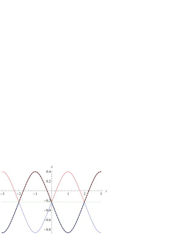
Figure 1: Plot of a periodic solution $z_{1,2}(t)$ of (18)–(21) with randomly chosen initial conditions. The solution has been redrawn such that $z_{1,2}(t)$ assumes its mean value (dotted line) at $t=0$. The black dashed curve represents the numerical solution $z_{1}(t)$ and the blue/red curves, partially hidden, the analytical solutions (31) according to the sign $\pm$.

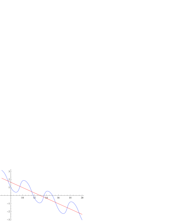
Figure 2: Plot of a numerical solution $\phi_{1}(t)$ of (18)–(21) with the same initial conditions as in figure 1. One notes a constant drift superimposed by a periodic oscillation.

As a function of the canonical coordinates $H$ assumes the form

$$H=\sqrt{1-z_{1}^{2}}\sqrt{1-z_{2}^{2}}\cos(\phi_{1}-\phi_{2})-2z_{1}z_{2}\;.$$ (22)

Then it follows that

$$\dot{\phi_{i}} = -\frac{\partial H}{\partial z_{i}}\;,i=1,2\;,$$ (23)

$$\dot{z_{i}} = \frac{\partial H}{\partial\phi_{i}}\;,i=1,2\;.$$ (24)

It can be shown that the solution $(\phi_{1}(t),z_{1}(t),\phi_{2}(t),z_{2}(t))$ of (18)-(21) moves on a $2$-dimensional torus defined by the equations ${\mathbf{S}}\cdot{\mathbf{e}}=s_{3}$ and $H=e$. Since the number of conserved quantities is half the phase space dimension the system (23), (24) is completely integrable in the sense of the Arnol’d–Liouville theorem A78 and its solution can be implicitly expressed in terms of integrals. In our case, these integrals are of elliptic kind and hence the solution can be explicitly given by means of Weierstrass elliptic functions ${\mathcal{P}}$ and elliptic integrals, see AS72 Ch. $17$ and $18$. We will give some more details of these calculations in Appendix B as well as a short introduction to the theory of elliptic integrals and functions in Appendix A. Here we will immediately formulate the final result for $z_{1,2}(t)$ after defining the quantities

$$g_{2} \equiv \frac{4}{27}\left(112e^{2}+16e\left(3s_{3}^{2}-16\right)+9s_{3}^{4}-168s_{3}^{2}+208\right),$$

$$g_{3} \equiv \frac{8}{729}\left(8e+3s_{3}^{2}-4\right)$$ (26)

$$\left(80e^{2}-48es_{3}^{2}-512e-9s_{3}^{4}-408s_{3}^{2}+560\right),$$

$$v_{\pm} \equiv \frac{1}{\pm 4\sqrt{(e-2)^{2}-3s_{3}^{2}}-8e-3s_{3}^{2}+4}\;,$$ (27)

$$u_{2} \equiv -\sqrt{3v_{+}}\;K\left(8\sqrt{(e-2)^{2}-3s_{3}^{2}}\;v_{+}\right)\;,$$ (28)

$${\mathcal{P}}(z) \equiv {\mathcal{P}}(z;g_{2},g_{3})\;,$$ (29)

$$P = 8\sqrt{v_{+}}K\left(\frac{v_{+}}{v_{-}}\right)\;,$$ (30)

$$z_{1,2}(t) = \frac{1}{2}\left(s_{3}\pm\sqrt{{\mathcal{P}}\left(\frac{it\sqrt{3}}{2}+u_{2}\right)-{\mathcal{P}}(u_{2})}\right)\;.$$ (31)

$K$ denotes the complete elliptic integral of first kind, see AS72 Ch. $17$. The sign $\pm$ in (31) has to be chosen to fit with $z_{1,2}(t)$ according to the initial conditions. $z_{1,2}(t)$ performs periodic oscillations about its mean value $\frac{s_{3}}{2}$ with period $P$ according to (30), see figure 1.

We now turn to the solution for $\phi_{1}(t)$. The conserved quantities (11), (12) can be used to express $\dot{\phi_{1}}$ solely in terms of $z_{1}$:

$$\dot{\phi_{1}}=\frac{(e-2)z_{1}+2s_{3}}{z_{1}^{2}-1}\;.$$ (32)

Since $z_{1}(t)$ is a periodic function, $\phi_{1}(t)$ will also be periodic in time, except for a constant drift that moves $\phi(t)$ with a certain amount $\delta\phi$ during one period $P$. This is illustrated in figure 2. Moreover, it turns out that $\frac{d\phi_{1}}{dz_{1}}$ can be written as a function of $z_{1}$ that is the quotient of a rational function and a square root of a polynomial of $4$th degree. Hence $\phi_{1}(z_{1})$ is expressible in terms of elliptic integrals and, after inserting $z_{1}(t)$, an explicit form of $\phi_{1}(t)$ is possible, analogously for $\phi_{2}(z_{2})$. We defer the details and the final result to Appendix C.

II.3 Solutions close to the ground states

The configuration $({\mathbf{s}}_{1},{\mathbf{s}}_{2})$ with minimal energy (13) under the constraints $|{\mathbf{s}}_{1}|^{2}=|{\mathbf{s}}_{2}|^{2}=1$ is a critical point of (13), i. e. , it satisfies the conditions

$$-\nabla_{{\mathbf{s}}_{1}}H = 3{\mathbf{s}}_{2}\cdot{\mathbf{e}}\;{\mathbf{e}}-{\mathbf{s}}_{2}=\lambda_{1}\;{\mathbf{s}}_{1}\;,$$ (33)

$$-\nabla_{{\mathbf{s}}_{2}}H = 3{\mathbf{s}}_{1}\cdot{\mathbf{e}}\;{\mathbf{e}}-{\mathbf{s}}_{1}=\lambda_{2}\;{\mathbf{s}}_{2}\;,$$ (34)

where $\lambda_{1},\;\lambda_{2}$ are Lagrange parameters due to the constraints. Upon forming the scalar product of both equations with ${\mathbf{e}}$ one easily derives the following alternative: Either ${\mathbf{s}}_{1}\cdot{\mathbf{e}}={\mathbf{s}}_{2}\cdot{\mathbf{e}}=0$ or $\lambda_{1}\lambda_{2}=4$ and ${\mathbf{s}}_{i}=\pm{\mathbf{e}},\;i=1,2$. In the first case, $H={\mathbf{s}}_{1}\cdot{\mathbf{s}}_{2}\geq-1$, whereas in the second case the function $H$ assumes the ground state energy $h_{0}=-2$ if ${\mathbf{s}}_{1}={\mathbf{s}}_{2}=\pm{\mathbf{e}}$. Hence the two ferromagnetic configurations parallel to ${\mathbf{e}}$ constitute the ground states of the dipole pair.

The energy barrier between the two ground states has the value $\Delta E=1$. This can be seen as follows. Any path $\pi$ in phase space joining the two ground states has at least one local energy maximum of height $h(\pi)$. The minimum $h_{1}$ of $h(\pi)$ among all such paths $\pi$ is necessarily assumed at a saddle point and hence at a critical point of (13). From the above classification of critical points only the possibilities ${\mathbf{s}}_{1}\cdot{\mathbf{e}}={\mathbf{s}}_{2}\cdot{\mathbf{e}}=0$ remain as candidates for saddle points and in this set only the configurations with ${\mathbf{s}}_{1}=-{\mathbf{s}}_{2}$ assume the minimal energy $h_{1}=-1$. Hence $\Delta E=h_{1}-h_{0}=1$.

For energies slightly above $h_{0}=-2$ it is sensible to linearize the eqm. Writing

$${\mathbf{s}}_{1} = \left(\begin{array}[]{l}X_{1}\\ X_{2}\\ -1\end{array}\right)+{\mathcal{O}}(|{\mathbf{X}}|^{2})\;,$$ (38)

$${\mathbf{s}}_{2} = \left(\begin{array}[]{l}X_{3}\\ X_{4}\\ -1\end{array}\right)+{\mathcal{O}}(|{\mathbf{X}}|^{2})\;,$$ (42)

we obtain the linearized eqm in the form

$$\dot{\mathbf{X}}(t)=A\;{\mathbf{X}}(t)\;,$$ (43)

where ${\mathbf{X}}=(X_{1},X_{2},X_{3},X_{4})$. The matrix $A$ has the form

$$A=\left(\begin{array}[]{cccc}0&2&0&1\\ -2&0&-1&0\\ 0&1&0&2\\ -1&0&-2&0\end{array}\right)\;,$$ (44)

and its eigenvalues are $\pm i,\pm 3i$. For later purposes we write down the first two components of the solutions of (43) using the initial conditions $X_{i}(0)=x_{i},\;i=1,\ldots,4$.

$$X_{1}(t) = \frac{1}{2}\left((x_{1}-x_{3})\cos(t)+(x_{2}-x_{4})\sin(t)+\right.$$ (45)

$$\left.(x_{1}+x_{3})\cos(3t)+(x_{2}+x_{4})\sin(3t)\right)\;,$$

$$X_{2}(t) = \frac{1}{2}\left((x_{2}-x_{4})\cos(t)+(x_{3}-x_{1})\sin(t)+\right.$$ (46)

$$\left.(x_{2}+x_{4})\cos(3t)-(x_{1}+x_{3})\sin(3t)\right)\;.$$

From this we can calculate the lowest non-trivial order of

$$z_{1}(t) = \pm\,\sqrt{1-(X_{1}(t)^{2}+X_{2}(t)^{2})}$$ (47)

$$= -1+\frac{1}{2}(X_{1}(t)^{2}+X_{2}(t)^{2})+{\mathcal{O}}(|{\mathbf{X}}|^{4})$$

$$= -1+\frac{1}{4}\left((x_{1}^{2}+x_{2}^{2}+x_{3}^{2}+x_{4}^{2})+\right.$$

$$\left(x_{1}^{2}+x_{2}^{2}-x_{3}^{2}-x_{4}^{2}\right)\cos(2t)+$$

$$\left.2(x_{1}x_{4}-x_{2}x_{3})\sin(2t)\right)+{\mathcal{O}}(|{\mathbf{X}}|^{4})\;.$$ (49)

At first sight it is remarkable that $z_{1}(t)$ contains no term proportional to $\sin(6t)$ or $\cos(6t)$ as one would expect from the possible addition of frequencies in $X_{1}(t)^{2}+X_{2}(t)^{2}$. However, the result (49) is in accordance with the low energy limit of the exact solution (29) of $z_{1}(t)$. Hence in the low energy limit ${\mathbf{s}}_{1}(t)$ performs a harmonic oscillation with the two angular frequencies $\omega_{1}=1$ and $\omega_{2}=3$ in the $x-y-$plane and $\omega_{3}=2$ in the $z-$direction. Recall that according to (7) we have chosen the unit of angular frequency to be $\omega_{0}$.

III Thermodynamics

A direct experimental test of the results of section D for nanomagnets is naturally affected by thermal fluctuations due to finite temperatures. Hence it seems worth while to investigate the thermodynamics of magnetic dipoles, especially to calculate thermodynamic functions such as the specific heat and the susceptibility. Furthermore, we will consider the autocorrelation function ($ac$) in the low temperature limit. The theoretical results will be compared with those of simulations of the system of two magnetic dipoles coupled to a heat bath. The methods used are described in the following subsection.

III.1 Methods

As it is well-known, thermodynamic functions such as the specific heat and the susceptibility can be derived from the partition function $Z(\beta)$ of the system. However, we were not able to explicitly calculate $Z(\beta)$ for the Hamiltonian (12). Fortunately, there exist powerful approximation schemes to overcome this difficulty. On the one hand it is possible to derive the moments of $H$ and thus the complete high temperature expansion (HTE) series of $Z(\beta)$. A large order truncation ($n=100$) together with an appropriate Padé approximation then yields very accurate approximations of $Z(\beta)$ and hence of the specific heat $c(\beta)$ down to low temperatures. On the other hand, the integrals over the $4$-dimensional phase space defining $Z(\beta)$ can be transformed conveniently to allow for a low temperature asymptotic expansion (LTA) of several orders of, say, $n=12$. The domains of validity of the two approximations, HTE and LTA, overlap, therefore together provide an accurate approximation of $c(\beta)$ without any need of interpolation.

Analogous remarks apply to the zero field susceptibility $\chi(\beta)$. Here it is possible to combine the complete HTE series with an LTA of several orders. Since the easy axis susceptibility $\chi(T)$ diverges for $T\rightarrow 0$ with the power $T^{-1}$ it is more appropriate to plot the product $T\;\chi(T)$ as a function of $T$. In contrast to this, the hard axis susceptibility approaches a finite value for $T\rightarrow 0$. The investigation of the autocorrelation function $ac$ and its thermal average $\langle ac\rangle$ combines dynamical and thermodynamical aspects of the system under consideration. As mentioned above, we will restrict ourselves to the low temperature asymptotic expansion up to terms of first order in $T$. In this realm it is sufficient to consider the solutions of the eqm close to the ground states, see subsection II.3, and to perform the integrations within the “harmonic oscillator approximation", i. e. an approximation of the Hamiltonian that is quadratic in the deviations from the ground state.

Furthermore, we have used classical spin dynamics and Monte Carlo simulations in order to compare our analytical derivations with numerical results.

III.2 Partition function

III.2.1 LTA

As a first step we derive the low temperature asymptotic expansion (LTA) of the partition function $Z(\beta)$, where $\beta$ is the dimensionless inverse temperature

$$\beta=\frac{E_{0}}{k_{B}T}\;,$$ (50)

and the energy unit $E_{0}$ has been defined in (13). We will also use the dimensionless temperature $\frac{k_{B}\,T}{E_{0}}$ which again will be denoted by $T$ without danger of confusion. According to its definition,

$$Z(\beta) = \frac{1}{(4\pi)^{2}}\int_{-1}^{1}dz_{1}\int_{-1}^{1}dz_{2}\int_{0}^{2\pi}d\phi_{1}\int_{0}^{2\pi}d\phi_{2}e^{-\beta H}.$$

For fixed $\phi_{2}$ we substitute $\phi_{1}=\phi+\phi_{2}$ and obtain the partial integral

$${\mathcal{I}}_{1} \equiv \int_{0}^{2\pi}d\phi_{1}\int_{0}^{2\pi}d\phi_{2}\;e^{-\beta H}$$

$$= 2\pi e^{2\beta z_{1}z_{2}}\int_{0}^{2\pi}d\phi\;e^{-\beta\sqrt{(1-z_{1}^{2})(1-z_{2}^{2})}\cos\phi}$$

$$= (2\pi)^{2}e^{2\beta z_{1}z_{2}}I_{0}\left(\beta\sqrt{(1-z_{1}^{2})(1-z_{2}^{2})}\right)\;,$$ (52)

where $I_{n}$ is the modified Bessel function of $n$th order. Next we substitute $z_{i}=-1+u_{i}^{2},\;u_{i}\geq 0,\;i=1,2,$ and obtain

$$Z(\beta) = \int_{0}^{\sqrt{2}}u_{1}du_{1}\int_{0}^{\sqrt{2}}u_{2}du_{2}$$ (53)

$$\exp\left(2\beta(-1+u_{1}^{2})(-1+u_{2}^{2})\right)$$

$$I_{0}\left(2\beta u_{1}u_{2}\sqrt{(1-\frac{1}{2}u_{1}^{2})(1-\frac{1}{2}u_{2}^{2})}\right)\;.$$

Now we consider the limit $\beta\rightarrow\infty$ by introducing polar coordinates $u_{1}=\frac{r}{\sqrt{\beta}}\cos\psi,\;u_{2}=\frac{r}{\sqrt{\beta}}\sin\psi,$ extracting the factor $e^{2\beta}/\beta^{2}$ and evaluating the remaining integral only in $0$th order of its Taylor series in $\beta^{-1}$. The domain of integration is extended to the whole first quadrant. This gives the contribution to $Z$ in the limit $\beta\rightarrow\infty$ from the neighborhood of the ground state $z_{1}=z_{2}=-1$. In order to include the equal contribution from the ground state $z_{1}=z_{2}=1$ we have to insert a factor $2$. We thus obtain the following asymptotic limit

$$Z(\beta) \sim \frac{2\,e^{2\beta}}{\beta^{2}}\int_{0}^{\infty}r^{3}\,e^{-2r^{2}}\,dr$$ (54)

$$\int_{0}^{\pi/2}d\psi\frac{1}{2}\sin(2\psi)I_{0}(r^{2}\sin(2\psi))$$

$$= \frac{2\,e^{2\beta}}{\beta^{2}}\int_{0}^{\infty}r^{3}\,e^{-2r^{2}}\frac{\sinh(r^{2})}{2r^{2}}\,dr$$ (55)

$$= \frac{e^{2\beta}}{6\beta^{2}}\;.$$ (56)

The method can be extended to obtain the first terms of an asymptotic series expansion for $Z(\beta)$. We omit the details and state the following result:

$$Z(\beta) \sim e^{2\beta}\left(\frac{1}{6\beta^{2}}+\frac{1}{9\beta^{3}}+\frac{1}{6\beta^{4}}+\frac{11}{27\beta^{5}}+\frac{227}{162\beta^{6}}\right).$$

III.2.2 HTE

Let us denote by $\mbox{Tr}(f)$ the integral of a function $f$ over $4$-dimensional phase space divided by its volume $(4\pi)^{2}$. Then the HTE of $Z(\beta)$ reads

$$Z(\beta)=\mbox{Tr}\left(e^{-\beta H}\right)=\sum_{n=0}^{\infty}\frac{(-\beta)^{n}}{n!}\,\mbox{Tr}(H^{n})\;,$$ (58)

where $H$ is the Hamiltonian (13). With the aid of computer algebraic software we calculate the moments $\mbox{Tr}(H^{n})$ and hence the HTE of $Z(\beta)$ with the result

$$Z(\beta)=\sum_{n=0}^{\infty}\frac{4^{n}\,F\left(1,-n;\frac{1}{2}-n;\frac{1}{4}\right)(-\beta)^{2n}}{(2n+1)^{2}(2n)!}\;,$$ (59)

where $F(a,b;c;z)$ denotes the hypergeometric function, see AS72 , ch. $15$. Since $\lim_{n\rightarrow\infty}F\left(1,-n;\frac{1}{2}-n;\frac{1}{4}\right)=\frac{4}{3}$ the radius of convergence of (59) is the same as that of the exponential series, namely $r=\infty$. Perhaps this explains the high quality of the approximations schemes based on (59).

III.3 Specific heat

According to the definition of the dimensionless specific heat

$$c(\beta)=\beta^{2}\;\frac{\partial^{2}}{\partial\beta^{2}}\;\log Z(\beta)\;,$$ (60)

the approximations of $Z(\beta)$ based on HTE and LTA can be transferred to $c(\beta)$. Especially, we apply a symmetric Padé approximation to the truncation of its HTE of order $n=100$ . This coincides with a $12-$th order LTA of $c(T)$, the first five terms of which are

$$c(T)=2+\frac{4}{3}T+\frac{14}{3}T^{2}+\frac{608}{27}T^{3}+\frac{10810}{81}T^{4}+\ldots\;,$$ (61)

in the domain $0<T<0.08$ up to a relative deviation of $2\times 10^{-3}$ , see figure 3. Alternatively, the specific heat can be obtained by numerically calculating the fluctuations of the (dimensionless) total energy $E$ according to

$$c^{*}(T)=\frac{1}{T^{2}}\left(\left<E^{2}\right>-\left<E\right>^{2}\right)\;$$ (62)

by means of Monte Carlo simulations.

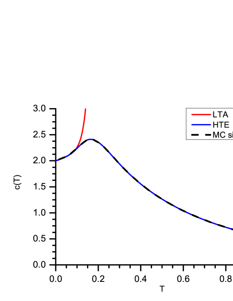
Figure 3: Plot of the specific heat $c(T)$ vs. $T$. The red curve shows the LTA up to order $T^{12}$; the blue curve is the result of using a $(50,50)$-Padé approximant based on the HTE of $c(\beta)$. Both curves coincide for $0<T<0.08$ with a maximal relative deviation of $2\times 10^{-3}$. The black dashed curve shows the results from our Monte Carlo simulation.

III.4 Susceptibility

III.4.1 Easy axis

The dimensionless zero field susceptibility for infinitesimal magnetic fields in the direction ${\mathbf{e}}$ joining the two dipoles (the “easy axis") is defined by

$$\chi(\beta)=\beta\langle S_{3}^{2}\rangle=\beta\frac{\mbox{Tr}\left(S_{3}^{2}\,\exp(-\beta H)\right)}{Z(\beta)}\;.$$ (63)

The HTE of the numerator is

$$\mbox{Tr}\left(S_{3}^{2}\,\exp(-\beta H)\right)=\sum_{n=0}^{\infty}\mbox{Tr}(S_{3}^{2}H^{n})\frac{(-\beta)^{n}}{n!}\;.$$ (64)

Again we can explicitly determine all moments occurring in (64)

$$\mbox{Tr}(S_{3}^{2}H^{m})=$$

$$\left\{\begin{array}[]{ll}\frac{2^{2n+1}\,F\left(1,-n;-n-\frac{1}{2};\frac{1}{4}\right)}{4n(n+2)+3}&\mbox{if }m=2n,\\ -\frac{2^{2n+1}\left(n\,F\left(1,1-n;\frac{1}{2}-n;\frac{1}{4}\right)+4n+2\right)}{(2n+1)(2n+3)^{2}}&\mbox{if }m=2n+1.\end{array}\right.\\$$ (65)

and perform an HTE approximation of $T\chi(T)$ analogously to that of the specific heat. The LTA of $T\chi(T)$ has been calculated up to $12-$th order, the first six terms being

$$T\chi(T)=4-\frac{16}{3}T-\frac{14}{9}T^{2}-\frac{140}{27}T^{3}-\frac{1628}{81}T^{4}-\frac{23888}{243}T^{5}-\ldots$$ (66)

The combination of HTE and LTA results yields the form of $T\chi(T)$ displayed in figure 4. By means of Monte Carlo simulations, we obtain the dimensionless susceptibility by evaluating the fluctuations of the total magnetization according to

$$\chi^{*}(T)=\frac{1}{T}\left(\left<{\mathbf{M}}^{2}\right>-\left<{\mathbf{M}}\right>^{2}\right).$$ (67)

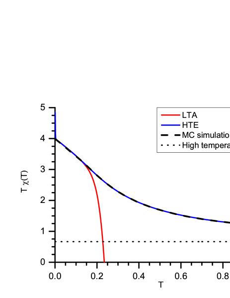
Figure 4: Plot of the product $T\chi(T)$ vs. $T$ for the easy axis. The red curve shows the LTA up to order $T^{12}$; the blue curve is a $(50,50)$-Padé approximation based on the HTE of $\chi(\beta)$. Both curves coincide for $0.01<T<0.06$ with a maximal relative deviation of $10^{-6}$. The black dashed curve shows the results from our Monte Carlo simulation. The dashed line represents the high temperature limit $2/3$ of $T\chi(T)$.

It is interesting to note that in contrast to the specific heat the susceptibility at very low temperatures cannot be determined correctly by using the standard Metropolis algorithm. As a result of the dipolar interaction an inherent easy-axis anisotropy in the direction of the connecting line between the two dipoles is formed resulting in a bi-stable system. As pointed out in section II.3 at low temperatures the two dipoles are fluctuating around their two possible ferromagnetic ground states that are separated by an energy barrier of $\Delta E=1$. During the timescale of a typical computer simulation the two dipoles will be trapped in one of the directions; any attempt to change both dipoles from one ground state configuration to the other is rejected in most cases leading to non-ergodic behavior. This is demonstrated in figure 5. In contrast to the analytical results (blue curve) the numerically determined susceptibility drops to zero for temperatures $T<0.1$.

This can be understood from the following argumentation: According to equation (67) we expect $T\chi\to 4$ for $T\to 0$, because of the $z$-component of the total magnetization $M_{z}=1+1$ or $M_{z}=-1-1$ for each of the ground states ($M_{x}$ and $M_{y}$ are both zero). This is the variance (fluctuation) of the total magnetization M since $\langle\textbf{M}\rangle=0$ in the ground state. The latter is only valid in a simulation if both ground states are equally often generated such that the average of M becomes 0. If the system gets trapped in one of the ground states we find $\langle\textbf{M}\rangle=\pm 2$ and hence the variance vanishes according to $T\chi=4-2\cdot 2=0$.

In order to obtain correct results we have used the so-called Exchange Monte Carlo method H96 in which many replicas of the system with different temperatures are simultaneously simulated and a virtual process exchanging configurations of these replicas is introduced. This exchange process allows the system at low temperatures to escape from a local minimum, hence leading to ergodic behavior and therefore producing correct data for the susceptibility (shown as red symbols in figure 5).

Furthermore, it is interesting to note that the specific heat can be obtained correctly by a standard Monte Carlo algorithm. In contrast to the susceptibility which is calculated using the fluctuations of a directed property, e. g. the total magnetization, the specific heat is calculated by sampling the fluctuations of the undirected total energy. Hence, the low temperature fluctuations in one of the two possible (degenerate) ground states are sufficient to yield the correct statistics.

The same argumentation using the fluctations of a directed property holds for the simulation of the hard axis susceptibility (see subsection III D 2). However, for this direction there is no energy barrier blocking the system.

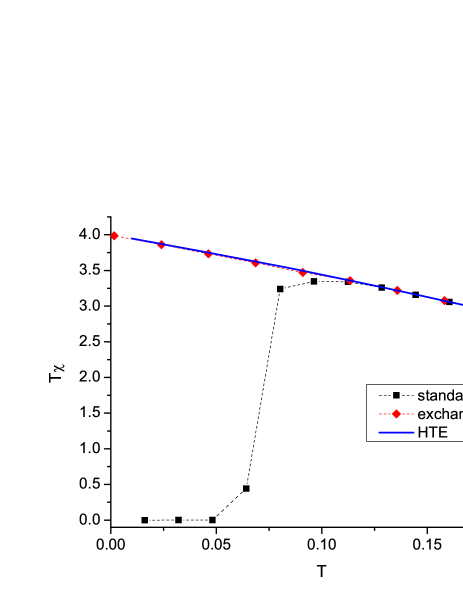
Figure 5: Plot of the product $T\chi(T)$ vs. $T$ for the easy axis. The blue curve shows the Padé approximation based on the HTE of $\chi(\beta)$. For $T<0.1$ the standard Monte Carlo simulation (black symbols) produces wrong results due to the non-ergodic behavior of the bi-stable dipole system whereas the exchange Monte Carlo method (red symbols) reproduces the analytical results.

III.4.2 Hard axis

The zero field susceptibility for the infinitesimal magnetic field in a direction perpendicular to the line joining the two dipoles (the “hard axis") will be calculated by the same methods as for the easy axis. Without loss of generality we choose the $x$-axis as the hard axis. Again we can explicitly determine all relevant moments

$$\mbox{Tr}(S_{1}^{2}H^{m})=$$

$$\left\{\begin{array}[]{l}\frac{2^{2n+1}\left(-(3n+5)\,F\left(1,-n;-n-\frac{1}{2};\frac{1}{4}\right)+4n+6\right)}{4n(n+2)+3}\quad\mbox{ if }m=2n\,,\\ \frac{9\times 2^{2n+1}\left((3n+5)\,F\left(1,n+\frac{3}{2};n+1;4\right)+n+1\right)\Gamma\left(n+\frac{3}{2}\right)-i\sqrt{3\pi}(3n+5)n!}{18(2n+3)\Gamma\left(n+\frac{5}{2}\right)}\\ \mbox{if }m=2n+1.\end{array}\right.\\$$ (68)

and obtain from this the HTE of the susceptibility and a corresponding $(50,50)$-Padé approximant that can be used down to low temperatures of, say, $T=0.01$. The LTA leads to the terms

$$\chi(T)=\frac{2}{3}-\frac{2}{9}T-\frac{2}{27}T^{2}-\frac{14}{81}T^{3}+{\mathcal{O}}(T^{4})\;.$$ (69)

Both approximations can be combined and yield a result that is very close to that obtained by Monte Carlo simulations, see figure 6. It is physically plausible that a small magnetic field in $x$-direction only leads to a small additional magnetization relative to that of the ground state. Hence the susceptibility is expected to approach a finite value for $T\rightarrow 0$. This is confirmed by the above result for the LTA (69). For the same reason the complications in the Monte Carlo simulations mentioned above, see section III.4.1, do not occur.

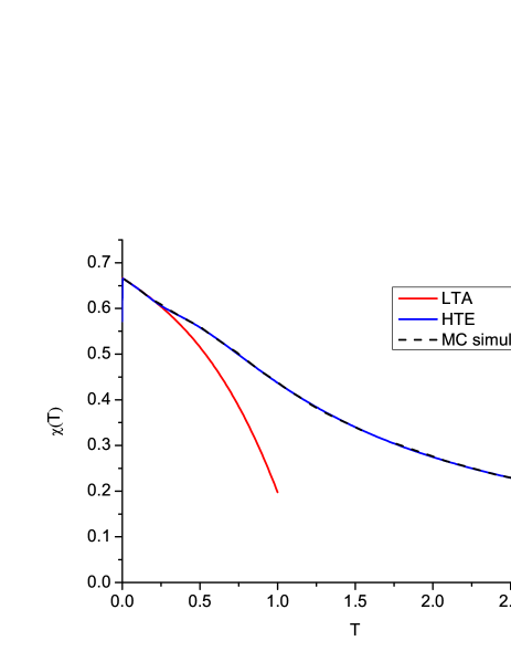
Figure 6: Plot of the hard axis susceptibility $\chi(T)$ vs. $T$. The blue curve shows the Padé approximation based on the HTE of $\chi(\beta)$, the red curve the LTA according to (69), and the black dashed curve the result of the Monte Carlo simulation.

III.5 Autocorrelation function

The autocorrelation function $ac$ or rather its thermal average $\langle ac\rangle$ provide typical characteristics of a system under the influence of thermal fluctuations. In our case we consider $ac={\mathbf{s}}_{1}(0)\cdot{\mathbf{s}}_{1}(t)$ (the result for the second dipole would be identical) and will exactly evaluate $\langle ac\rangle$ in the limit $\beta\rightarrow\infty$. From section II.3 we know already that only the three frequencies $\omega_{1}=1,\;\omega_{2}=3$ and $\omega_{3}=2$ will occur in the Fourier spectrum of low temperature oscillations. Since

$$ac = \sqrt{(1-z_{1}(0)^{2})(1-z_{1}(t)^{2})}\cos(\phi_{1}(0)-\phi_{1}(t))$$ (70)

$$+z_{1}(0)z_{1}(t)\;,$$

we expect that the contribution $\langle z_{1}(0)z_{1}(t)\rangle$ will be suppressed by thermal averaging over all phase shifts of the $z_{1}$-oscillations. On the other hand, $\langle\sqrt{(1-z_{1}(0)^{2})(1-z_{1}(t)^{2})}\cos(\phi_{1}(0)-\phi_{1}(t))\rangle$ will probably not vanish since the phase shifts of the $x-y$-oscillations have been already canceled in the argument of the $\cos$-function. This conjecture has to be confirmed by the detailed calculations.

These calculations can be simplified by the following consideration. The transformation ${\mathbf{s}}_{i}\mapsto-{\mathbf{s}}_{i},\;i=1,2,$ introduces a minus sign in the eqm (9) and hence can be considered as a kind of “time reversal". However, it leaves the $ac$ invariant and hence $\langle ac\rangle$ will be also invariant under time reversal. Consequently, the terms of $ac$ proportional to $\sin(t),\sin(2t)$ and $\sin(3t)$ will vanish in the thermal average and need not be calculated.

The calculation of $\langle ac(t)\rangle$ is based on the approximation of the Hamiltonian $H$ to terms at most quadratic in the deviations from a ground state. We do not give the details but the main steps are sketched in Appendix D. The final result reads:

$$\langle ac\rangle=1-\frac{4}{3\beta}+\frac{3\cos(t)+\cos(3t)}{3\beta}+{\mathcal{O}}(\beta^{-2})\;.$$ (71)

This shows that indeed the frequency $\omega=2$ of the $z_{1}$-oscillation is suppressed by thermal averaging and can at most occur as contributions of order ${\mathcal{O}}(\beta^{-2})$.

We compared these results with numerical simulations. In order to calculate the canonical ensemble average numerically we used the so-called “Gibbs approach" LL99 , where the trajectories ${\mathbf{s}}_{1}(t)$ for the dipoles are calculated for the isolated system by solving the equations of motion (9) and (10) over a certain number of time steps numerically. The initial conditions for each trajectory are generated by a standard Monte Carlo simulation for a temperature $T$. By averaging all generated trajectories at each time step one obtains the canonical ensemble average. In figure 7 we show a comparison of our analytical and simulation results in the time domain. The Fourier transform of the simulation data (see figure 8) yields the expected spectrum showing three distinct peaks, where the peak at the frequency $\omega=2$ is almost suppressed compared to the other peaks.

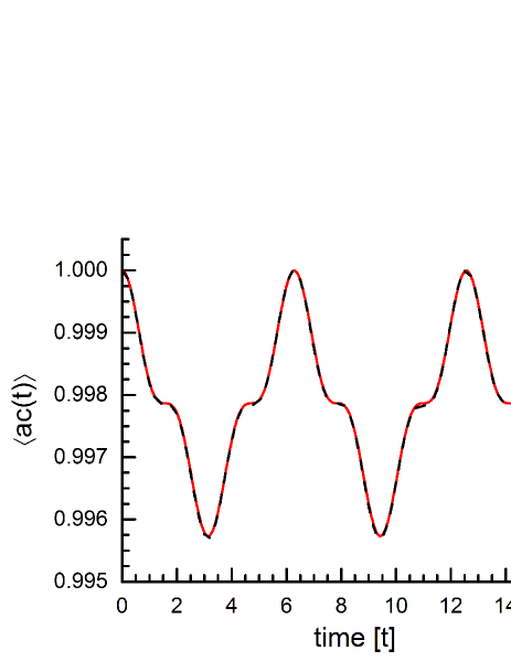
Figure 7: Plot of the autocorrelation function $\langle ac(t)\rangle$ vs. $t$ for a dimensionless temperature of $T=0.00160156$. The red curve shows the analytical results; the black curve shows the numerical results.

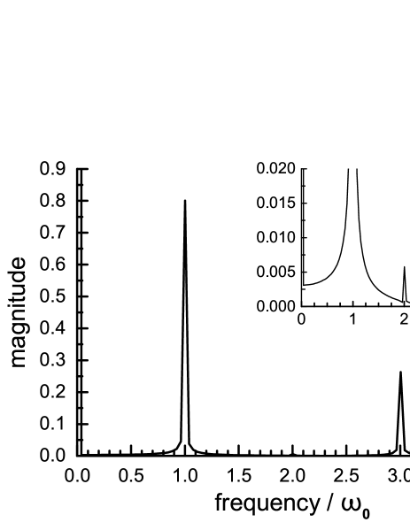
Figure 8: Plot of the Fourier transform of the autocorrelation function $\langle ac(t)\rangle$ vs. $\omega$ for a dimensionless temperature of $T=0.00160156$. The inset shows the peak at $\omega=2$ which is almost suppressed by thermal averaging. The amplitudes of the two large peaks are in the ratio of $2.95:1$ in accordance with (71).

IV Summary and Outlook

In this paper we have investigated the system consisting of two magnetic dipoles, fixed in space and interacting via its magnetic fields. The dynamics of this system has been completely resolved and the general solution of the equations of motion has been given in terms of elliptic integrals and Weierstrass elliptic functions. The thermodynamics of the two dipole system based on the canonical ensemble has also been determined by means of series expansions, including the low temperature limit of the autocorrelation function. The analytical results have been confirmed by numerical Monte Carlo simulations.

Hence we have found a simple but non-trivial example for a solvable system in the sense of classical mechanics and of classical thermodynamics for systems with small particle numbers. The other motif of our studies was to prepare the investigation of larger systems of interacting dipoles that have been recently realized by experimentalists. Therefore it is in order to reflect about possible generalizations of our methods to larger systems. First, it is clear that the Hamiltonian (22) can be directly generalized to systems of $N$ dipoles and yields the corresponding Hamiltonian eqm for the canonical coordinates $(p_{i},\,q_{i})=(\phi_{i},\,z_{i}),\;i=1,\ldots,N$. However, we do not expect that these eqm are completely integrable for $N>2$ due to the lack of a sufficient number of integration constants. Nevertheless, it might be possible to find some exact solutions for larger systems of dipoles and to identify its ground states. In particular, the linearization of the eqm close to the ground state(s) should be possible and would only be practically limited by the size of $N$. Concerning thermodynamics, we are pessimistic about the possibility to generalize our series expansions to larger systems due to the complexity of the calculations. However, the “linear oscillator approximation" would still be possible and would yield low temperature limits of, e. g. , the autocorrelation function. In view of these difficulties the role of numerical simulations would become more important for larger systems of magnetic dipoles.

Appendix A Elliptic integrals and Weierstrass elliptic functions

There are many problems in theoretical physics that lead to elliptic integrals (EI) or their inverses, elliptic functions (EF). We only mention a few:

• Various problems of classical mechanics B09 including one-dimensional motion of a particle in a cubic or quartic potential, the spherical pendulum or the spinning top,

• the magnetic field of a circular current loop J99 , Ch. 5,

• the TE field in a slab filled with a Kerr non-linear medium S95 ,

• certain solutions of the Korteweg-de-Vries equation B09 , and

• problems from cosmology AW10 .

Nevertheless, most authors of physics textbooks seem to refrain from the use of these special functions, one exception being the above-cited J99 . This is the more regrettable since by utilizing computer algebra software both EI and EF can be evaluated with the same ease as, say, the $\sin$ and $\arcsin$ functions.

Here we cannot give an extended introduction into the field but will rather sketch the fundamental ideas. One can understand the EI and EF as generalizations of the well-known “circular case", where one encounters the elementary integral

$$t=\int\;\frac{dx}{\sqrt{1-x^{2}}}=\arcsin x\;+\,t_{0}\;,$$ (72)

defined for $-1\leq x\leq 1$ and its inverse function

$$x(t)=\sin(t-t_{0})\;,$$ (73)

that can be extended to a periodic function defined for all $-\infty<t<\infty$. The following generalization of (72) is the incomplete EI of the first kind:

$$t=\int_{0}^{x}\;\frac{dx}{\sqrt{(1-x^{2})(1-mx^{2})}}\equiv F(\arcsin x,m)\;.$$ (74)

By the complete EI of the first kind one denotes the special case of the integral

$$\int_{0}^{1}\;\frac{dx}{\sqrt{(1-x^{2})(1-mx^{2})}}\equiv K(m)\;,$$ (75)

that can be used, e. g. , for calculating the period of oscillation of a pendulum.

More generally, it can be shown A78 , Ch. 17, that any integral of a rational function of $x$ and $\sqrt{P(x)}$, where $P(x)$ is a polynomial of at most $4$th degree, can be expressed in terms of elementary functions and the so-called EI of first, second or third kind.

Similarly as in the circular case, one is often interested in the function $x(t)$ rather than $t(x)$, that is, for the periodic extension of the inverse function of the EI, the EF. There exist different versions of the EF; in this paper we will use the Weierstrass EF, $u={\mathcal{P}}(z;g_{2},g_{3})$. It is first defined by inverting

$$z=\int_{\infty}^{u}\;\frac{dv}{\sqrt{P(v)}}\;,$$ (76)

where $P(v)=4v^{3}-g_{2}v-g_{3}$. Then ${\mathcal{P}}$ is extended to a doubly periodic complex function, analytic in the whole complex plane except for the pole at $z=0$ and its translates. For more details, see Chapter $18$ of A78 and an introduction to the theory as it is given, e. g. , in B09 or B61 .

Appendix B Exact solution for $z_{1}(t)$

The first step is to eliminate $z_{2}$ and $\phi_{1}-\phi_{2}$ from (20) by using the constants ${\mathbf{S}}\cdot{\mathbf{e}}=s_{3}$ and $H=e$. We write $z_{1}=z$. The result is

$$\dot{z} = \sqrt{-3Q_{+}Q_{-}}\;,$$ (77)

where

$$Q_{\pm} \equiv \frac{1}{3}\left(1-2e-3s_{3}z+3z^{2}\pm\sqrt{e^{2}-4e-3s_{3}^{2}+4}\right).$$

Upon substituting

$$v = (2z-s_{3})^{2}-v_{0}\;,$$ (79)

$$v_{0} \equiv \frac{2}{9}\left(8e+3s_{3}^{2}-4\right)$$ (80)

we obtain

$$t=\int\frac{dz}{\sqrt{-3Q_{+}Q_{-}}}=\frac{2}{\sqrt{-3}}\int\frac{dv}{\sqrt{4v^{3}-g_{2}v-g_{3}}}\;,$$ (81)

with $g_{2}$ and $g_{3}$ according to (LABEL:DS7a) and (26). Inserting appropriate boundaries and writing $4v^{3}-g_{2}v-g_{3}=P(v)$ we have

$$\frac{i\sqrt{3}}{2}t = \int_{-v_{0}}^{(2z-s_{3})^{2}-v_{0}}\frac{dv}{\sqrt{P(v)}}\;,$$ (82)

$$= \int_{\infty}^{(2z-s_{3})^{2}-v_{0}}\frac{dv}{\sqrt{P(v)}}-\int_{\infty}^{-v_{0}}\frac{dv}{\sqrt{P(v)}}$$ (83)

$$\equiv u_{1}-u_{2}\;.$$ (84)

According to the definition of the Weierstrass ${\mathcal{P}}$-function, this is equivalent to

$${\mathcal{P}}(u_{1}) = (2z-s_{3})^{2}-v_{0}\;,$$ (85)

$$= (2z-s_{3})^{2}+{\mathcal{P}}(u_{2})\;,$$ (86)

or, solving for $z$,

$$z(t) = \frac{1}{2}\left(s_{3}\pm\sqrt{{\mathcal{P}}(u_{1})-{\mathcal{P}}(u_{2})}\right)\;,$$ (87)

$$= \frac{1}{2}\left(s_{3}\pm\sqrt{{\mathcal{P}}\left(\frac{i\sqrt{3}}{2}t+u_{2}\right)-{\mathcal{P}}(u_{2})}\right)\;.$$ (88)

This confirms (31). As a consequence of choosing the lower boundary of the integral (82) to be $-v_{0}$ we have $z(0)=s_{3}/2$. For a more general solution one can simply replace $t$ in the r. h. s. of (88) by $t-t_{0}$.

Appendix C Exact solution for $\phi_{1,2}(t)$

We write $z=z_{1,2},\;\phi=\phi_{1,2}$ and have to solve the integral

$$\int d\phi=\int\frac{\dot{\phi}}{\dot{z}}dz\;,$$ (89)

where $\dot{\phi}$ and $\dot{z}$ have to be inserted from (32) and (77).
Defining

$$a_{0} = -s_{3}\sqrt{-3v_{-}}\;,$$ (90)

$$a_{1} = 2\sqrt{-3v_{-}}\;,$$ (91)

$$\mu = \frac{1}{16}\left(4e+s_{3}^{2}+4\right)\left(4e+3s_{3}^{2}-4\right)\;,$$ (92)

$$m = \frac{v_{+}}{v_{-}}\;,$$ (93)

the substitution $x=a_{1}\,z+a_{0}$ yields

$$\frac{dz}{\dot{z}}=\frac{dz}{\sqrt{-3Q_{+}Q_{-}}}=\frac{dx}{a_{1}\sqrt{\mu}\sqrt{\left(1-x^{2}\right)\left(1-mx^{2}\right)}}\;.$$ (94)

Upon this substitution (32) can be written as

$$\dot{\phi}=\frac{(e-2)z+2s_{3}}{z^{2}-1}=\frac{A_{+}}{1-n_{+}x}+\frac{A_{-}}{1-n_{-}x}\;,$$ (95)

where

$$A_{\pm} = \frac{-2+e\mp 2s_{3}}{\pm 2+s_{3}}\;,$$ (96)

$$n_{\pm} = \mp\frac{1}{\sqrt{-3v_{-}}(2\pm s_{3})}\;.$$ (97)

These transformations lead to writing (89) as a sum of two integrals of the form

$$W\left(n;\left.x\right|m\right)\equiv\int\frac{dx}{(1-nx)\sqrt{\left(1-x^{2}\right)\left(1-mx^{2}\right)}}\;.$$ (98)

Writing

$$\frac{1}{(1-nx)}=\frac{1}{1-n^{2}x^{2}}+\frac{n\,x}{1-n^{2}x^{2}}\;,$$ (99)

we obtain

$$W\left(n;\left.x\right|m\right)=$$

$$\Pi\left(n^{2};\left.\sin^{-1}(x)\right|m\right)+$$

$$\frac{n}{\sqrt{n^{2}-1}\sqrt{m-n^{2}}}\tan^{-1}\left(\frac{\sqrt{z^{2}-1}\sqrt{m-n^{2}}}{\sqrt{mz^{2}-1}\sqrt{n^{2}-1}}\right)\;,$$

(100)

where $\Pi$ is the incomplete elliptic integral of third kind, see AS72 Ch.17. The final result hence reads

$$\phi(t)=\phi_{0}+\frac{1}{a_{1}\sqrt{\mu}}\times$$

$$\left(A_{+}W\left(n_{+};\left.\frac{z(t)-a_{0}}{a_{1}}\right|m\right)+A_{-}W\left(n_{-};\left.\frac{z(t)-a_{0}}{a_{1}}\right|m\right)\right).$$ (101)

Appendix D Low temperature limit of $\langle ac(t)\rangle$

For the calculation of the low temperature limit of $\langle ac(t)\rangle$ we write for the magnetic moments close to one of the ground states, analogously to (38) and (42),

$${\mathbf{s}}_{1} = \left(\begin{array}[]{l}X_{1}\\ X_{2}\\ -1+\frac{1}{2}(X_{1}^{2}+X_{2}^{2})\end{array}\right)\;,$$ (105)

$${\mathbf{s}}_{2} = \left(\begin{array}[]{l}X_{3}\\ X_{4}\\ -1+\frac{1}{2}(X_{3}^{2}+X_{4}^{2})\end{array}\right)\;,$$ (109)

and evaluate $H$ up to second order in $|{\mathbf{X}}|$. The result can be written as

$$H_{2}\equiv-2+{\mathbf{X}}\cdot{\mathbf{M}}\cdot{\mathbf{X}}\;,$$ (110)

where

$${\mathbf{M}}=\left(\begin{array}[]{cccc}1&0&\frac{1}{2}&0\\ 0&1&0&\frac{1}{2}\\ \frac{1}{2}&0&1&0\\ 0&\frac{1}{2}&0&1\end{array}\right)\;.$$ (111)

The eigenvalues of the symmetric matrix ${\mathbf{M}}$ are $M_{1,2}=\frac{3}{2},\;M_{3,4}=\frac{1}{2}$. They are positive in accordance with the fact that the considered ground state realizes the energy minimum $h_{0}=-2$. Their values are exactly $1/2$ of the two basic frequencies $\omega_{1}=1,\;\omega_{2}=3$, i. e. , of the absolute values of the eigenvalues of $A$, see (44). We perform a rotation into the eigenbasis of ${\mathbf{M}}$ and call the new coordinates $Y_{i},\,i=1,\ldots,4$. In the second order approximation w. r. t. $|{\mathbf{X}}|$ we then obtain the partition function

$$\frac{1}{2}Z(\beta)\sim e^{2\beta}\frac{1}{(4\pi)^{2}}\prod_{i=1}^{4}\int_{-\infty}^{\infty}\exp\left(-\beta M_{i}Y_{i}^{2}\right)\,dY_{i}=\frac{e^{2\beta}}{12\beta^{2}}\;,$$ (112)

which confirms the result (56) obtained by a different method. Recall that the factor $\frac{1}{2}$ is introduced since the second ground state gives the same contribution to $Z(\beta)$.

The present method is also suited to calculate the low temperature limit of $\langle ac(t)\rangle$. Consider first

$$ac_{1}(t) \equiv X_{1}(0)\,X_{1}(t)=\frac{1}{2}(Y_{2}-Y_{4})\times$$

$$(-Y_{1}\sin 3t+Y_{3}\sin t+Y_{2}\cos 3t-Y_{4}\cos t).$$

If this expression is inserted into the integrals (112) only those terms survive that are quadratic in the $Y_{i}$, namely $\frac{1}{2}\left(Y_{2}^{2}\cos 3t+Y_{4}^{2}\cos t\right)$. Upon division by $\frac{1}{2}Z(\beta)$ we obtain

$$\langle ac_{1}(t)\rangle=\frac{2}{3\beta}\cos^{3}t+{\mathcal{O}}(\beta^{-2})\;.$$ (114)

By azimuthal symmetry $\langle ac_{2}(t)\rangle\equiv\langle X_{2}(0)\,X_{2}(t)\rangle=\langle ac_{1}(t)\rangle$. For $\langle ac_{3}(t)\rangle$ we have

$$\langle ac_{3}(t)\rangle \equiv \langle\quad(-1+\frac{1}{2}(X_{1}(0)^{2}+X_{2}(0)^{2}))\times$$ (116)

$$(-1+\frac{1}{2}(X_{1}(t)^{2}+X_{2}(t)^{2}))\quad\rangle$$

$$= 1-\frac{1}{2}\langle(X_{1}(0)^{2}+X_{2}(0)^{2})\rangle$$

$$-\frac{1}{2}\langle(X_{1}(t)^{2}+X_{2}(t)^{2})\rangle+{\mathcal{O}}(\beta^{-2})$$

and by the same method as above it follows that the thermal average of the time-dependent terms vanishes such that

$$\langle ac_{3}(t)\rangle=-\frac{4}{3\beta}+{\mathcal{O}}(\beta^{-2})\;.$$ (117)

Adding all contributions to $\langle ac(t)\rangle$ we obtain the following expression which proves (71):

$$\langle ac(t)\rangle = 1-\frac{4}{3\beta}+\frac{4}{3\beta}\cos^{3}t+{\mathcal{O}}(\beta^{-2})$$

$$= 1-\frac{4}{3\beta}+\frac{3\cos(t)+\cos(3t)}{3\beta}+{\mathcal{O}}(\beta^{-2}).$$

References

- (1) M. Ewerlin, D. Demirbas, F. Brüssing, O. Petracic, A.A. Ünal, S. Valencia, F. Kronast, and H. Zabel, Phys. Rev. Lett., 110, 177209, 2013
- (2) G. Miloshevich, T. Dauxois, R. Khomeriki, and S. Ruffo, Eur. Phys. Lett., 104, 17011, 2013
- (3) M. Varon, M. Beleggia, T. Kasama, R.J. Harrison, R.E. Dunin-Borkowski, V.F. Puntes, C. Frandsen, Sci. Rep., 3, 1234, 2013
- (4) S.A. Dzyan and B.A. Ivanov, Low Temp. Phys., 39, 525–529, 2013
- (5) S.A. Dzyan and B.A. Ivanov, JETP, 116, 975–979, 2013
- (6) B. Wunsch, N.T. Zinner, I.B. Mekhov, S.-J. Huang, D.-W. Wang, and E. Demler, Phys. Rev. Lett., 107, 073201, 2011
- (7) J. Stuhler, A. Griesmaier, T. Koch, M. Fattori, T. Pfau, S. Giovanazzi, P. Pedri, and L. Santos, Phys. Rev. Lett., 95, 150406, 2005
- (8) T. Unold, K. Mueller, Ch. Lienau, T. Elsaesser, and A.D. Wieck, Phys. Rev. Lett., 94, 137404, 2005
- (9) T. Jonsson, P. Nordblad, and P. Svedlindh, Phys. Rev. B, 57, 497–594, 1998
- (10) R.F. Wang, C. Nisoli, R.S. Freitas, J. Li, W. McConville, B.J. Cooley, M.S. Lund, N. Samarth, C. Leighton, V.H. Crespi, P. Schiffer, Nature, 439, No. 7074, 303-306, 2006
- (11) C. Castelnovo1, R. Moessner, and S.L. Sondhi, Nature, 451, 06433, 2008
- (12) K. Hiroi, K. Komatsu, T. Sato, Phys. Rev. B, 83, No. 22, 224423, 2011
- (13) A. Imre, G. Csaba, L. Ji, A. Orlov, G.H. Bernstein, and W. Porod, Science, 311, No. 5758, 205-208, 2006
- (14) I. Eichwald, S. Breitkreutz, G. Ziemys, G. Csaba, W. Porod, and M. Becherer, Nanotechnology, 25, 335202, 2014
- (15) A. Campa, T. Dauxois, and S. Ruffo, Phys. Rep., 480, 57, 2009
- (16) K. Hukushima and K. Nemoto, J. Phys. Soc. Jpn., 65, 1604-1608, 1996
- (17) V.I. Arnol’d, Mathematical Methods of Classical Mechanics, Springer, Berlin, 1978
- (18) M. Abramowitz and I.A. Stegun, (eds.) Handbook of Mathematical Functions, Dover, New York, 1972
- (19) M. Luban and J. H. Luscombe, Am. J. Phys., 67, 1161, 1999
- (20) A.J. Brizard, Eur. J. Phys., 30, 729-750, 2009
- (21) J.D. Jackson, Classical electrodynamics, 3rd ed. , Wiley, Hoboken, 1999.
- (22) H.-W. Schürmann, Z. Phys., B 97, 515-522, 1995
- (23) J. D´Ambroise and F.L. Williams, J. Math. Phys., 51, 062501, 2010
- (24) F. Bowman, Introduction to elliptic functions, Dover, New York, 1961