A Time-Triggered Constraint-Based Calculus for Avionic Systems

Abstract

The Integrated Modular Avionics (IMA) architecture and the Time-Triggered Ethernet (TTEthernet) network have emerged as the key components of a typical architecture model for recent civil aircrafts. We propose a real-time constraint-based calculus targeted at the analysis of such concepts of avionic embedded systems. We show our framework at work on the modelisation of both the (IMA) architecture and the TTEthernet network, illustrating their behavior by the well-known Flight Management System (FMS).

I Introduction

The growing complexity of avionic embedded systems led to the definition of a new standard of architecture called Integrated Modular Avionics (IMA) [1]. This type of architecture is characterized essentially by the sharing of distributed computing resources, called modules. Sharing these resources requires to guarantee some safety properties such as the collision-free. In order to achieve this objective, the Avionic Full Duplex Switched Ethernet (AFDX) [2] has been adopted as a networking standard for the avionic systems. IMA and AFDX became the components of a typical architecture model for the recent civil aircrafts such as the Boeing $B787$ and the Airbus $A380$. However, AFDX underuses the physical capacities of the network. Recently, the Time-Triggered Ethernet (TTEthernet) has emerged as a new standard of the avionic network [3]. This standard enables to achieve a best usage of the network and is more deterministic since the schedule is established offline.

Both IMA and TTEthernet segregate mixed-criticality components into partitions for a safer integration. IMA enables applications to interact safely by partitioning them spatially (memory zones) and temporally (processor schedules) over distributed Real-Time Operating Systems (RTOS). TTEthernet, on the other hand, allows these distributed RTOS to communicate safely with each other by partitioning bandwidth into time slots (network schedules).

Although a considerable effort has recently been devoted for the validation of TTEthernet (e.g. [16, 6]), to the best of our knowledge the analysis and validation of TTEthernet usage in model-based development for the integration on IMA has been so far relatively ignored. The present paper proposes a framework which empowers us to analyze, as well as provide guidelines and some mechanism design principles for IMA integration through TTEthernet network, exploiting notions and techniques from Concurrent Constraint Programming (CCP) formalism.

CCP [25, 23] is a well-established formalism for reasoning about concurrent and distributed systems. It is a matured model of concurrency with several reasoning techniques (e.g. [21, 9, 5]) and implementations (e.g. [24, 26, 14]). It is adopted in a wide spectrum of domains and applications such as biological phenomena, reactive systems and physical systems. It enjoys a dual view of processes as agents interacting with one another and as logical formulas allowing to benefit from both the well-established process calculi and logic formalisms. CCP is a powerful way to define complex synchronization schemes in concurrent and distributed settings parametric in a constraint system. This provides a very flexible way to tailor data structures to specific domains and applications. We refer the reader to [18] for a recent survey on ccp-based models.

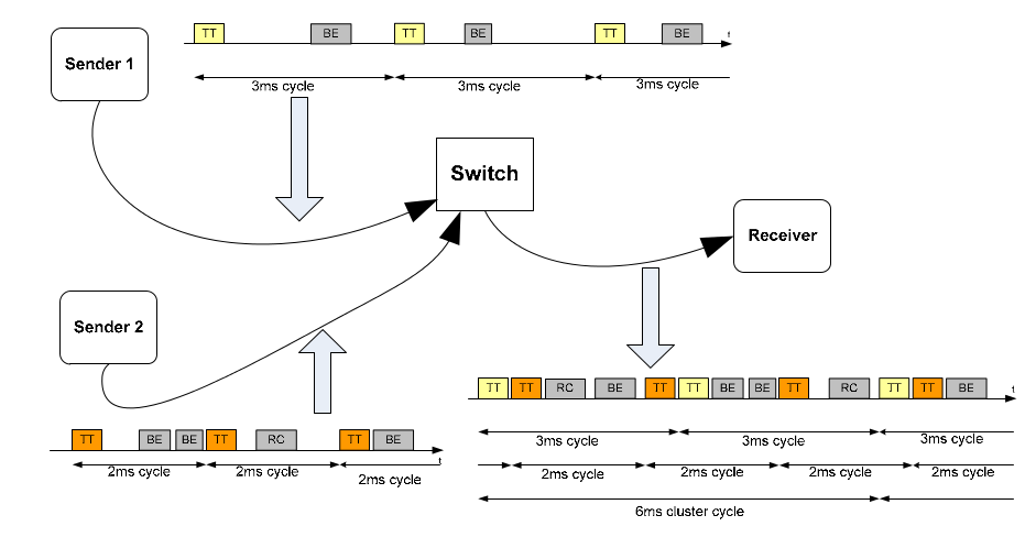
Figure 1: [3] Example of a Time-Triggered Ethernet network

Drawing on earlier work on timed ccp-based formalisms [22, 17], in the present paper we introduce a calculus to provide a formal basis for the analysis of time-triggered architectures in avionic embedded systems. Like its predecessors, our calculus is built around a small number of primitive operators or combinators parametric in a constraint system. It extends the Timed Concurrent Constraint Programming (tcc) [22] in order to define infinite periodic behaviors specific to IMA and TTEthernet and to comply with the requirements of time triggered processes. We then demonstrate the pertinence of this calculus by an elegant modeling of the concepts related to the IMA and TTEthernet architectures. Finally, we illustrate these concepts by modeling a subsystem of the well-known flight management system.

To our knowledge, the present paper is the first to provide a comprehensive framework for the behavioral analysis for IMA systems deployed throughout a TTEthernet network. Previous process algebraic models do not deal with both IMA and TTEthernet [8, 27, 19], or only accounted for the IMA concept without providing a comprehensive set of reasoning techniques for the verification of the requirements of avionic systems. Similarly, existing formal calculi such as the Network Calculus [13] and the Real-Time Calculus [20] fall short of accounting for the time triggered architecture while maintaining a good accuracy in specifying the system designs [15].

The rest of the paper is organized as follows: in §II we fix some basic notations, briefly revise the concepts of IMA and TTEthernet architectures, and introduce the flight management system; in §III we present our conceptual framework; §IV, §V and §VI deliver our core technical contribution: the modelisation of IMA systems deployed throughout a TTEthernet network; §VII contains our concluding remarks.

II Preliminaries

This section briefly revises the concepts of IMA and TTEthernet architectures which underpin the work in this paper. It also introduces the flight management system, a leading example used to illustrate our conceptual framework.

II-A Integrated Modular Avionics

The main idea underlying the concept of IMA architecture [4] is the sharing of resources between some functions while preventing any interference between them. Resource sharing reduces the cost of large volume of wiring and equipment while the non interference guarantee is required for safety reasons.

The IMA architecture is a modular real-time architecture for avionic systems defined in ARINC653 [1]. Each functionality of the system is implemented by one or a set of functions distributed across different modules. A module represents a processor where many functions can be executed. Functions deployed on the same module may have different criticality levels. For safety reasons, the functions must be strictly isolated using partitions. The partitioning of these functions is two dimensional: spatial partitioning and temporal partitioning. The spatial partitioning is implemented by assigning statically all the resources for the partition being executed in a module and no other partition can have the access to the same resources at the same time. The temporal partitioning is rather implemented by allocating a periodic time window dedicated for the execution of each partition.

II-B Time-Triggered Ethernet

Ethernet uses an event-triggered transfer principle where an end system can access the network at arbitrary points in time. Service to the end systems is on a first come, first serve basis which, unfortunately, can substantially increase transmission delay and jitter when several end systems need to communicate over the same shared medium. Time-Triggered Ethernet [3] (TTEthernet) specifies time-triggered services that are added to the standards for Ethernet established in IEEE STD 802.3-2005. In contrast to event-triggered transfer principle, the time-triggered transfer principle uses a network-wide synchronized time base to coordinate between end systems, which limits latency and jitter. As depicted in Figure 1, TTEthernet enables time-triggered and event-triggered communication, as well as integrated time-triggered/event-triggered communication on the same physical network. TTEthernet limits latency and jitter for time-triggered (TT) traffic, limits latency for rate-constrained (RC) traffic, while simultaneously supporting the best-effort (BE) traffic service of IEEE 802.3 Ethernet. This allows application of Ethernet as a unified networking infrastructure. In this paper, however, we shall consider only time-triggered traffic (TT).

As depicted in Figure 2, the physical topology of a TTEthernet network is a graph $\mathbf{G}(\mathcal{V},\mathcal{E})$, where end systems and switches are vertices $\mathcal{V}$ and the physical links connecting vertices are edges $\mathcal{E}$. Each physical link connecting two vertices defines two directed ”dataflow links”. The set of dataflow links is denoted $\mathcal{L}$. We denote by $[v_{1},v_{2}]$ the dataflow link from vertex $v_{1}$ to vertex $v_{2}$ and by

$$p=[[v_{1},v_{2}],[v_{2},v_{3}],\cdots[v_{m-2},v_{m-1}],[v_{m-1},v_{m}]]$$

the dataflow path connecting one end system (the sender) $v_{1}$ to exactly one other end system (the receiver) $v_{m}$. In Figure 2, a path from A to F is depicted by the dotted line. In accordance with the Ethernet convention, information between the sender and receiver is communicated in form of messages $f_{i}$ called frames. $\mathcal{F}$ denotes the set of all frames. Frames may be delivered from a sender to multiple receivers where the individual dataflow paths between the sender and each single receiver together form a ”virtual link“. Hence, a virtual link $vl$ is the union of the dataflow paths that link the sender to each receiver. An example of a virtual link from the sender A to the receiver F and G is shown in Figure 2. We denote by $\mathcal{D}\mathcal{P}$ (resp. $\mathcal{V}\mathcal{L}$) the set of dataflow paths (resp. virtual links).

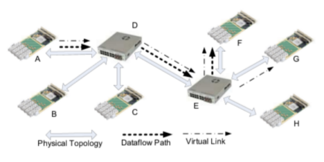
Figure 2: [28] A TTEthernet with six end systems and two switches connected in multi-hop

II-C Flight Management System

Now, we briefly recall a subsystem of the Flight Management System drawn from[12]. It controls the display of static navigation information in the cockpit screens and it is illustrated by Figure 3.

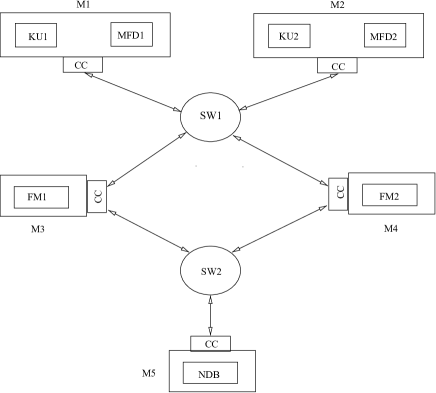
Figure 3: Flight Management System

Two partitions $\mbox{\emph{KU}}_{i}$ ($i=1;2$), the Keyboard and cursor Unit, handle the waypoint information requests of the pilot and the co-pilot. Each request is transmitted to $\mbox{\emph{FM}}_{1}$ and $\mbox{\emph{FM}}_{2}$, the two Flight Manager partitions. Each FM requests separately NDB, the Navigation DataBase, via an unicast communication to retrieve the waypoint information. Each $\mbox{\emph{FM}}_{i}$ ($i=1;2$) transmits the result to its associated $\mbox{\emph{MFD}}_{i}$, the Multi Functional Display partition, which displays the information on the corresponding screen. The dataflow inside this subsystem is summarized by Figure 4.

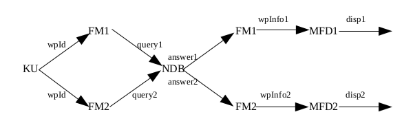
Figure 4: FMS dataflow

(R-Tell) $\frac{}{\langle\mathbf{tell}(c),d\rangle\longrightarrow\langle\mathbf{0},d\wedge c\rangle}$	(R-Ask-1) $\frac{d\vdash c}{\langle\mathbf{when}\ c\ \mathbf{do}\ P,d\rangle\longrightarrow\langle P,d\rangle}$	(R-Ask-2) $\frac{d\not\vdash c}{\langle\mathbf{when}\ c\ \mathbf{do}\ P,d\rangle\longrightarrow\langle\mathbf{0},d\rangle}$
$\begin{array}[]{ll}\mbox{(R-Par)}\ \frac{\langle P,d\rangle\longrightarrow\langle P^{\prime},d_{p}^{\prime}\rangle\ \ \langle Q,d\rangle\longrightarrow\langle Q^{\prime},d_{q}^{\prime}\rangle}{\langle P\;\|\;Q,d\rangle\longrightarrow\langle P^{\prime}\;\|\;Q^{\prime},d_{p}^{\prime}\wedge d_{q}^{\prime}\rangle}&\ \mbox{(R-Loc)}\ \frac{\langle P,c\wedge\exists xd\rangle\longrightarrow\langle P^{\prime},c^{\prime}\wedge\exists xd\rangle}{\langle(\mathbf{local}\ x;c)\ \mathbf{in}\ P,d\rangle\longrightarrow\langle(\mathbf{local}\ x;c^{\prime})\ \mathbf{in}\ P^{\prime},d\wedge\exists xc^{\prime}\rangle}\\[17.07164pt] \mbox{(R-Per)}\ \frac{}{\langle!_{T}P,d\rangle\longrightarrow\langle P\;\|\;\mathbf{next}^{T}(!_{T}P),d\rangle}&\ \mbox{(R-Def)}\ \frac{A(\tilde{x})\stackrel{{\scriptstyle\mbox{def}}}{{=}}P\ \ \langle P[\tilde{v}/\tilde{x}],d\rangle\longrightarrow\langle P^{\prime},d^{\prime}\rangle}{\langle A(\tilde{v}),d\rangle\longrightarrow\langle P^{\prime},d^{\prime}\rangle}\end{array}$
(R-Obs) $\frac{\langle P,c\rangle\longrightarrow^{\ast}\langle Q,d\rangle\not\longrightarrow\ \ F(Q)=R}{P\ \mbox{$\stackrel{{\scriptstyle(c,d)}}{{\Longrightarrow}}$}\ R}$

TABLE I: Internal transition rules $\longrightarrow$ (upper part) and the observable transition rule $\Longrightarrow$ (lower part).

III The ttcc Process Calculus

This section describes the syntax and the operational semantics of the Time-Triggered Concurrent Constraint Programming (ttcc). This calculus extends the Timed Concurrent Constraint Programming (tcc) [22] both syntactically and semantically. On the syntactic level, we add a new operator to define infinite periodic behaviors specific to IMA and TTEthernet. On the semantics level, we extend tcc model to comply with the requirements of time triggered processes. We start by recalling a fundamental notion in ccp-based calculi: constraint system.

III-A Constraint System

The ttcc model is parametric in a constraint system specifying the structure and interdependencies of information that processes can ask of and add to a central shared store. A constraint system provides a signature (a set of constants, functions and predicates symbols) from which constraints can be constructed as well as an entailment relation (a first order logic over the signature), denoted $\vdash$, which specifies the interdependancies between these constraints. Formally, a constraint system is a pair $(\Sigma,\Delta)$ where $\Sigma$ is a signature and $\Delta$ is a first order theory over $\Sigma$. Constraints are first-order formulas over $\mathcal{L}$, the underlying first-order language under $\Sigma$. We shall denote by $\mathcal{C}{\it onst}$ the set of constraints in the underlying constraint system with typical elements $c,d,\ldots$. Given two constraints (i.e. two pieces of information) $c$ and $d$, we say that $c$ entails $d$, and write $c\vdash d$, if and only if $c\Rightarrow d$ is true in all models of $\Delta$. In other words, $d$ can be deduced from $c$.

III-B Process Syntax

As shown in Figure 5, a common store is used as communication medium by ttcc processes to post and read constraints (viz. partial information). We use $\mathcal{P}{\it roc}$ to denote the set of all ttcc processes, with typical elements $P$, $Q$, $\ldots$. They are built from the following primitive operators:

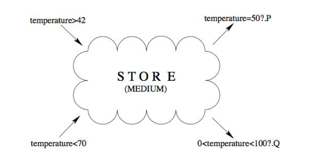
Figure 5: Processes communicating via a common store

$$P,Q,\ldots ::= \mathbf{0}$$

$$| \mathbf{tell}(c)$$

$$| \mathbf{when}\ c\ \mathbf{do}\ P$$

$$| P\;\|\;Q$$

$$| (\mathbf{local}\ x;c)\ \mathbf{in}\ P$$

$$| \mathbf{next}\ P$$

$$| !_{T}P$$

$$| A(\tilde{x})$$

The null process $\mathbf{0}$ does nothing. The process $\mathbf{tell}(c)$ adds constraint $c$ to the store within the current time. The process $\mathbf{when}\ c\ \mathbf{do}\ P$ executes $P$ if its guard constraint $c$ is entailed by the store in the current time. Otherwise, $P$ is discarded. $P\;\|\;Q$ represents $P$ and $Q$ acting concurrently. The process $(\mathbf{local}\ x;c)\ \mathbf{in}\ P$ behaves like $P$, except that it declares variable $x$ private to $P$ (its value is hidden to other processes). In $\mathbf{next}\ P$, the process $P$ will be activated in the next time unit. The operator $!_{T}$ is used to define infinite periodic behavior. $!_{T}P$ represents $P\;\|\;\mathbf{next}^{T}P\;\|\;\mathbf{next}^{2T}P\;\|\;\cdots$ where $\mathbf{next}^{T}P$ is the abbreviation of $\mathbf{next}\ (\mathbf{next}\ (\cdots(\mathbf{next}\ P)\cdots))$ where $\mathbf{next}$ is repeated $T$ times. The process $A(\tilde{x})$ is an identifier with arity $|\tilde{x}|$. We assume that every such an identifier has a unique (recursive) definition of the form $A(\tilde{x})\stackrel{{\scriptstyle\mbox{def}}}{{=}}P$.

III-C Operational Semantics

The dynamics of the calculus is specified by means of two transition relations between configurations $\longrightarrow,\Longrightarrow\subseteq\mathcal{C}{\it onf}\times\mathcal{C}{\it onf}$ obtained by the rules in Table I. A configuration is a pair $\langle P,d\rangle\in\mathcal{P}{\it roc}\times\mathcal{C}{\it onst}$ where $d$ represents the current store. $\mathcal{C}{\it onf}$ denote the set of all configurations with typical elements $\Gamma,\Gamma^{\prime},\ldots$.

An internal transition $\langle P,d\rangle\longrightarrow\langle P^{\prime},d^{\prime}\rangle$ means that $P$ under the current store $d$ evolves internally into $P^{\prime}$ and produces the store $d^{\prime}$ and corresponds to an operational step that take place during a time-unit. Rules in upper part of Table I define the internal transitions. Rule (R-Tell) means that a $\mathbf{tell}$ process adds information (viz. a constraint) to the current store and terminates. Rules (R-Ask) specify that the guard constraint of an ask process must be entailed by the current store when it is triggered. Note that it is different to the usual semantics of an ask process in timed ccp-based calculi. Our periodically time triggered scenario requires that the current store under which a process is triggered must entail its guard constraints. Otherwise, the process must be discarded in the current time and triggered again periodically. Rule (R-Par) specifies the concurrent execution of multiple processes and assumes maximal parallelism since, typically in avionic systems, agents running concurrently are located on different modules. In rule (R-Loc), the process $(\mathbf{local}\ x;c)\ \mathbf{in}\ P$ behaves like $P$, except that it binds the local variable inside $P$. Rule (R-Per) states that in $!_{T}P$, the process $P$ is activated in the current time and then repeated periodically. Finally, rule (R-Def) states that the identifier process $A(\tilde{x})$ behaves like $P$. Process $P[\tilde{v}/\tilde{x}]$ denotes $P$ where each variable $x_{i}\in\tilde{x}$ inside $P$ is substituted by the value $v_{i}\in\tilde{v}$.

In order to unfold the timed operator $\mathbf{next}$, we consider observable transitions. An observable transition $P\ \mbox{$\stackrel{{\scriptstyle(c,d)}}{{\Longrightarrow}}$}\ R$, means that the process $P$ under the current store $c$ evolves in one time-unit to $R$ and produces the store $d$. We say that $R$ is an observable evolution of $P$. Rule (R-Obs) in lower part of Table I defines the observable transitions. The transition $P\ \mbox{$\stackrel{{\scriptstyle(c,d)}}{{\Longrightarrow}}$}\ R$ is obtained from a finite sequence of internal transitions $\langle P,c\rangle\longrightarrow^{\ast}\langle Q,d\rangle\not\longrightarrow\mbox{ where }F(Q)=R$ and $F:\mathcal{P}{\it roc}\rightarrow\mathcal{P}{\it roc}$, the future function is defined as

$$F(Q)=\left\{\begin{array}[]{ll}\displaystyle Q^{\prime}&\mbox{if }Q=\mathbf{next}\;Q^{\prime},\\[8.53581pt] \displaystyle F(Q_{1})\;\|\;F(Q_{2})&\mbox{if }Q=Q_{1}\;\|\;Q_{2},\\[8.53581pt] \displaystyle(\mathbf{local}\ x;c)\ \mathbf{in}\ F(Q^{\prime})&\mbox{if }Q=(\mathbf{local}\ x;c)\ \mathbf{in}\ Q^{\prime},\\[8.53581pt] \displaystyle F(Q^{\prime})&\mbox{if }Q=A(\tilde{v})\mbox{ and }A(\tilde{v})\stackrel{{\scriptstyle\mbox{def}}}{{=}}Q^{\prime},\\[8.53581pt] \displaystyle\mathbf{0}&\mbox{otherwise.}\end{array}\right.$$

$\Gamma\not\longrightarrow$ means that there is no $\Gamma^{\prime}$ such that $\Gamma\longrightarrow\Gamma^{\prime}$.

IV Modeling the Integrated Modular Avionics

In this section, we illustrate our conceptual framework by modeling the IMA concept using the flight management system introduced in Section II-C. Throughout the rest of this paper, we shall consider the widely used Finite-Domain Constraint System $\mathbf{FD}[max]$ [11] where $\Sigma$ is given by the constants symbols $0,1,2,...,max-1$ and the relation symbols $=,\neq,<,\leq,>,\geq$. $\Delta$ is given by the axioms in Number Theory.

IV-A Partitions

We assume that each partition is a black box with an input satisfying some (application dependent) constraint $c$ and an output (viz. its result $r$) which is added to the (local) store by assigning it to the (local) variable $x$. Moreover, each partition (e.g. $KU$ depicted in Figure 6) is characterized by its offset $o$, duration $\tau$, and period $\pi$. Hence, we have the following definition:

$$P(o,\tau,\pi)\stackrel{{\scriptstyle\mbox{def}}}{{=}}$$

$$!_{\pi}\;(\mathbf{local}\;x,c_{p})\;\mathbf{in}\Bigl{(}\mathbf{next}^{o}\bigl{(}\mathbf{when}\;c\;\mathbf{do}\;\mathbf{next}^{\tau}\mathbf{tell}(x=r)\bigr{)}\Bigr{)}$$ (1)

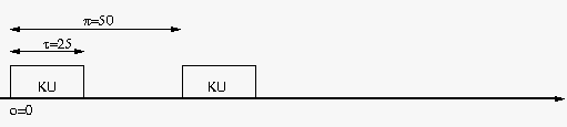
Figure 6: FMS’s Keyboard and Cursor Control Unit partition (KU)

Intuitively, the partition $P(o,\tau,\pi)$ starts its first execution after $o$ (its offset) time units, when the constraint $(\mathbf{when}\;c)$ on its input is checked. If the current store entails $c$ then the partition adds the constraint $x=r$ to the (local) store after $\tau$ time units, the duration of the partition. Then every $\pi$ period time, the partition is reactivated thanks to the $!_{\pi}$ operator. Note that we use $(\mathbf{local}\;x,c_{p})\;\mathbf{in}$ in the above definition only if we do not want the current execution of the partition to overwrite the result of its previous execution. In other words, the partition is in a queuing mode. Note that we could use streams [25] to represent changes in the value of $x$ instead of binding $x$ locally inside $\Bigl{(}\mathbf{next}^{o}\bigl{(}\mathbf{when}\;c\;\mathbf{do}\;\mathbf{next}^{\tau}\mathbf{tell}(x=r)\bigr{)}\Bigr{)}$.

Example

Consider the $KU$ partition modeling the Keyboard and Cursor Control Unit shown in Figure 6. Assume that whenever $KU$ is triggered, it checks whether or not the pilot requested the waypoint information modelled by the boolean variable $pReq$. If the pilot did make a request, $KU$ increment by one the waypoint ID. The $KU$ partition is then modelled by:

$$KU(0,25,50)\stackrel{{\scriptstyle\mbox{def}}}{{=}}$$

$$!_{50}\;\mathbf{when}\;(pReq=\mathbf{true})\;\mathbf{do}\;\mathbf{next}^{25}\;\mathbf{tell}(wpId=wpId+1)$$

since $\mathbf{next}^{0}\;P=P$.

IV-B Modules

Now, we move onto modeling modules. We start by introducing some auxiliary functions and notations. We define the projection functions $\sigma_{i}$ for any positive integer $i$, which given a vector $\tilde{x}=(x_{1},x_{2},\cdots,x_{n})$ returns $\sigma_{i}(\tilde{x})=x_{i}$ ($i\leq|\tilde{x}|$). We shall denote $s=(o,\tau,\pi)$ the scheduling parameters of a partition and by $\tilde{s}$ a vector of scheduling parameters ranged by their offset parameters.

The most important requirement about the scheduling is the contention-freedom property: mutual-exclusion of execution times of the partitions. Let

$$\mathbf{MAF}(\tilde{s})=\mathbf{LCM}\bigl{(}\{\sigma_{3}\bigr{(}\sigma_{i}(\tilde{s})\bigr{)}\;|\;1\leq i\leq|\tilde{s}|\}\bigr{)}$$

be the least common multiple of all partition periods of the scheduling $\tilde{s}$ which is commonly refereed as the MAjor time Frame. Given the scheduling vector $\tilde{s}$ of a module’s partitions, we say that $\tilde{s}$ is contention-free, denoted $\mathbf{CF}(\tilde{s})$, when the following holds.

$$\mathbf{CF}(\tilde{s})=\mathbf{true}\mbox{ iff }\forall 1\leq i\neq j\leq|\tilde{s}|,$$

$$\forall t_{i}\in\Bigl{[}0\cdot\cdot\Bigr{(}\frac{\mathbf{MAF}(\tilde{s})}{\sigma_{3}\sigma_{i}(\tilde{s})}-1\Bigl{)}\Bigr{]},\forall t_{j}\in\Bigl{[}0\cdot\cdot\Bigr{(}\frac{\mathbf{MAF}(\tilde{s})}{\sigma_{3}\sigma_{j}(\tilde{s})}-1\Bigl{)}\Bigr{]}:$$

$$\Bigr{(}t_{i}\times\sigma_{3}\sigma_{i}(\tilde{s})+\sigma_{1}\sigma_{i}(\tilde{s})\geq t_{j}\times\sigma_{3}\sigma_{j}(\tilde{s})+\sigma_{1}\sigma_{j}(\tilde{s})+\sigma_{2}\sigma_{j}(\tilde{s})\Bigl{)}\vee$$

$$\Bigr{(}t_{j}\times\sigma_{3}\sigma_{j}(\tilde{s})+\sigma_{1}\sigma_{j}(\tilde{s})\geq t_{i}\times\sigma_{3}\sigma_{i}(\tilde{s})+\sigma_{1}\sigma_{i}(\tilde{s})+\sigma_{2}\sigma_{i}(\tilde{s})\Bigl{)}$$ (2)

Now, given a scheduling vector $\tilde{s}$ of a module’s partitions, the module is defined as follows:

$$M(\tilde{s}) \stackrel{{\scriptstyle\mbox{def}}}{{=}} \mathbf{when}\;\mathbf{CF}(\tilde{s})\;\mathbf{do}\;\prod_{1\leq i\leq|\tilde{s}|}P_{i}\bigl{(}\sigma_{i}(\tilde{s})\bigr{)}$$ (3)

where each partition $P_{i}$ has an input satisfying some constraint $c_{i}$ and produces $r_{i}$ as its result. Both $c_{i}$ and $r_{i}$ are application dependent.

Informally, the module $M(\tilde{s})$ verifies that the scheduling of its partitions is well-defined, that is, the mutual-exclusion of partitions’ window execution times is satisfied. If the scheduling is well-defined, all the partitions are activated in the current time but due to the definition of partitions (see Section IV-A), each of them will actually be triggered at its own offset time.

Example

Consider the module $M1$ of the flight management system (see Figure 3). Assume that the scheduling parameters of its second partition (viz. $MFD1$ ) is $s_{MFD1}=(o=25,\tau=25,\pi=50)$, then it is easy to see that the scheduling vector $\tilde{s}_{M1}=(s_{KU1},s_{MFD1})$ satisfies the contention-freedom property (Equation (IV-B)).

$$M1(\tilde{s}_{M1}) \stackrel{{\scriptstyle\mbox{def}}}{{=}} \mathbf{when}\;\mathbf{CF}(s_{KU1},s_{MFD1})\;\mathbf{do}\;$$

$$KU1(s_{KU1})\;\|\;MFD1(s_{MFD1}).$$

IV-C IMA

An IMA system, is simply a product of multiple modules running concurrently and communicating throughout a TTEthernet network which we will address in the following section. Given an IMA system of $n$ modules $\{M_{1},M_{2},\cdots,M_{n}\}$, with $\tilde{s}_{i}$ the scheduling vector of $M_{i}$, we call IMA scheduler and denote by $\gamma_{IMA}=\{\tilde{s}_{i}:1\leq i\leq n\}$ the set of the scheduling vectors of all the modules composing the system. Table II shows an example of an IMA scheduler for the flight management system. Then, the whole IMA system is modelled as follows.

$$\mathbf{IMA}(\gamma_{IMA}) \stackrel{{\scriptstyle\mbox{def}}}{{=}} \prod_{1\leq i\leq|\gamma_{IMA}|}M_{i}(\tilde{s}_{i})$$ (4)

$$\begin{array}[]{|l|l|l|l|l|}\hline\cr\mbox{Partitions}&\pi&\tau&o&\mbox{Module}\\ \hline\cr\hline\cr\mbox{KU1 (MFD1)}&50&25&0\;(25)&\mbox{M1}\\ \hline\cr\mbox{KU2 (MFD2)}&50&25&0\;(25)&\mbox{M2}\\ \hline\cr\mbox{FM1}&60&30&7&\mbox{M3}\\ \hline\cr\mbox{FM2}&60&30&27&\mbox{M4}\\ \hline\cr\mbox{NDB}&100&20&77&\mbox{M5}\\ \hline\cr\end{array}$$

TABLE II: IMA-schedule

V Modeling TTEthernet

The modeling of the TTEthernet network will follow the same principle as in the previous section. We start by modeling tt-frames. Then we model dataflow links. Finally, in order to build the complete network, we piece together all datalinks if the temporal parameters of the frames satisfy all the temporal requirements of the TTEthernet.

V-A Frames

According to the aerospace standard AS6802 [3], a TT frame $f_{i}$ on a data link $[v_{k},v_{l}]$, denoted $f_{i}^{[v_{k},v_{l}]}$ is fully temporally specified by its offset time, length and period:

$$f_{i}^{[v_{k},v_{l}]}=(f_{i}^{[v_{k},v_{l}]}\cdot offset,f_{i}\cdot length,f_{i}\cdot period).$$

The length and the period of a frame are given a priori and remain fixed along the virtual link. It is the task of the tt-scheduler to assign values to the frame’s offset times on all dataflow links belonging to the frame’s virtual link. Note that these three temporal parameters are the same that fully characterize a partition on a module (see Section IV-A). Hence, there is a perfect similarity between partitions on a module and frames on a dataflow link. Therefore, we model a frame $f_{i}^{[v_{k},v_{l}]}=(o,\tau,\pi)$ by the following process:

$$F_{i}^{[v_{k},v_{l}]}(o,\tau,\pi)\stackrel{{\scriptstyle\mbox{def}}}{{=}}$$

$$!_{\pi}\;(\mathbf{local}\;x,c_{i})\;\mathbf{in}\Bigl{(}\mathbf{next}^{o}\bigl{(}\mathbf{when}\;c\;\mathbf{do}\;\mathbf{next}^{\tau}\mathbf{tell}(x=r)\bigr{)}\Bigr{)}$$ (5)

where $o=f_{i}^{[v_{k},v_{l}]}\cdot offset$, $\tau=f_{i}\cdot length$, and $\pi=f_{i}\cdot period$. Again, $(\mathbf{local}\;x,c_{i})\;\mathbf{in}$ is used only if the tt-frame is transmitted under a queuing mode.

Example

Consider the waypoint ID $wpId$ produced by the $KU$ partition in the previous section. Assume that it is transmitted along the dataflow link $[M1,SW1]$ w.r.t. the tt-scheduling parameters $(50,2,10)$. Then under a sampling mode, $wpId$ along $[M1,SW1]$ is modelled as follows.

$$WPID1^{[M1,SW1]}(50,2,10)\stackrel{{\scriptstyle\mbox{def}}}{{=}}$$

$$!_{10}\;\mathbf{next}^{50}\;\mathbf{when}\;(wpId1>0)\;\mathbf{do}\;\mathbf{next}^{2}\mathbf{tell}(sw11=wpId1)$$

We use the guard constraint $(wpId>0)$ so that the waypoint ID is transmitted only when the pilot’s request is processed by $KU1$.

V-B Dataflow link

Exploiting the temporal characterization similarity between tt-frames and IMA partitions, we naturally model dataflow links the same way we modelled modules. Indeed, like partitions on the same module, the temporal parameters of tt-frames transmitted along the same dataflow link must satisfy the contention freedom property given by Equation (IV-B). Therefore, given $\tilde{\varsigma}^{[v_{i},v_{j}]}$, the tt-scheduling vector of frames tranallowssmitted along the dataflow link $[v_{i},v_{j}]$, we model the dataflow link by the following process.

$$L^{[v_{i},v_{j}]}(\tilde{\varsigma}^{[v_{i},v_{j}]}) \stackrel{{\scriptstyle\mbox{def}}}{{=}} \mathbf{when}\;\mathbf{CF}(\tilde{\varsigma}^{[v_{i},v_{j}]})\;\mathbf{do}$$ (6)

$$\prod_{1\leq i\leq|\tilde{\varsigma}^{[v_{i},v_{j}]}|}F_{i}^{[v_{i},v_{j}]}\bigl{(}\sigma_{i}(\tilde{\varsigma}^{[v_{i},v_{j}]})\bigr{)}$$

$$\begin{array}[]{|l|l|l|l|l|}\hline\cr\mbox{Frames}&\pi&\tau&o&\mbox{Datalink}\\ \hline\cr\hline\cr\mbox{wpId1}&10&2&50&\mbox{[M1,SW1]}\\ \hline\cr\mbox{wpId2}&10&2&50&\mbox{[M2,SW1]}\\ \hline\cr\mbox{wpId1 (wpId2)}&10&2&55\;(53)&\mbox{[SW1,M3]}\\ \hline\cr\mbox{wpId1 (wpId2)}&10&2&55\;(53)&\mbox{[SW1,M4]}\\ \hline\cr\mbox{query1}&30&3&40&\mbox{[M3,SW2]}\\ \hline\cr\mbox{query2}&30&3&60&\mbox{[M4,SW2]}\\ \hline\cr\mbox{query11(query2)}&30&3&44\;(41)&\mbox{[SW2,M5]}\\ \hline\cr\end{array}$$

TABLE III: TT-scheduler

allows

Example

consider the dataflow link $[SW1,M3]$ which transmits both frames $wpId1$ and $wpId2$ from the switch $SW1$ to the module $M1$. From the TT-scheduling parameters given in Table III, we have that $\tilde{\varsigma}^{[SW1,M3]}=\bigl{(}(55,2,10),(53,2,10)\bigr{)}$, which satisfies the contention-freedom property (IV-B).

$$\begin{array}[]{lll}L^{[SW1,M3]}\Bigl{(}(55,2,10),(53,2,10)\Bigr{)}&\stackrel{{\scriptstyle\mbox{def}}}{{=}}&\\ \lx@intercol\;\;\mathbf{when}\;\mathbf{CF}\Bigl{(}\bigl{(}(55,2,10),(53,2,10)\bigr{)}\Bigr{)}\;\mathbf{do}\hfil\lx@intercol\\ \lx@intercol\;\;WPID1^{[SW1,M3]}(55,2,10)\;\|\;WPID2^{[SW1,M3]}(53,2,10).\hfil\lx@intercol\end{array}$$

V-C The network

Now that we have built each dataflow link separately, we need to piece them together in order to obtain the full network. However, unlike the IMA modules which operate independently from each other, dataflow links form paths and virtual links and hence their combination must satisfy some specific constraints. In this paper, we will illustrate two of them: a path dependent constraint and a virtual link dependent one. For the complete list of these constraints and their formalization, we refer to [7, 28].

Well-formed path

within the dataflow path of a frame the dispatch points in time on two adjacent datalinks will be well-timed. Formally,

$$\forall p\in\mathcal{D}\mathcal{P},\forall[v_{x},v_{y}],[v_{y},v_{z}]\in p,$$

$$(f_{i}^{[v_{y},v_{z}]}.offset)-(f_{i}^{[v_{x},v_{y}]}.offset)\geq max(\emph{hopdelay})$$ (7)

where $max(\emph{hopedelay})$ is an off-line configurable upper bound of the maximum latency over a single hop.

For example, assume that $max(\emph{hopedelay})=3$, then the $wpId1$ frame’s path $p=[[M1,SW1],[SW1,M3]]$ from $M1$ to module $M3$, whose temporal parameters are given in Table III, is well-formed. We have

$$WPID1^{[SW1,M3]}\cdot offset \geq WPID1^{[M1,SW1]}\cdot offset$$

$$+\;max(\emph{hopedelay})$$

since $55\geq 50+3$.

Simultaneous relay

an avionic functionality might require that some frames to be simultaneously dispatched on all outgoing dataflow links of the relaying nodes within their virtual links. Given a virtual link $vl$ of a frame $f_{i}$, the simultaneous relay requirement is satisfied if the following holds.

$$\forall p_{k},p_{l}\in vl\;(k\neq l),\forall[v_{x},v_{y}]\in p_{k},\forall[v_{x},v_{z}]\in p_{l},$$

$$(f_{i}^{[v_{x},v_{y}]}.offset)=(f_{i}^{[v_{x},v_{z}]}.offset)$$ (8)

For example, the switch $SW1$ dispatches simultaneously the waypoint ID frames on both $[SW1,M3]$ and $[SW1,M4]$ datalinks (see the tt-scheduler in Table III).

We are ready to build the full network. Let $\mathbf{WF}$ and $\mathbf{SR}$ denote the predicates specifying the well-formed and the simultaneous-relay requirements respectively. Given $\tilde{\varsigma}_{TT}$, the tt-scheduler of the full network, we proceed as follows: first, we verify that $\tilde{\varsigma}_{TT}$ satisfies both $\mathbf{WF}$ and $\mathbf{SR}$ constraints; then we build each datalink of the network separately; finally we piece them together thanks to the parallel composition operator.

$$\mathbf{TTE}(\tilde{\varsigma}_{TT}) \stackrel{{\scriptstyle\mbox{def}}}{{=}} \mathbf{when}\;\bigl{(}\mathbf{WF}(\tilde{\varsigma}_{TT})\wedge\mathbf{SR}(\tilde{\varsigma}_{TT})\bigr{)}\;\mathbf{do}$$ (9)

$$\prod_{1\leq i\leq|\tilde{\varsigma}_{TT}|}L^{[v_{k},v_{l}]}_{i}\bigl{(}\sigma_{i}(\tilde{\varsigma}_{TT}^{[v_{k},v_{l}]})\bigr{)}$$

VI Modeling the full system

In Section IV and Section V we have built the IMA modules and the network independently. In order to piece them together, the IMA scheduler and the tt-scheduler must satisfy the latency constraints which ensure that some avionic functions produce their responses within some given deadlines. There are two types of latency: the elementary latency and the end-to-end latency as depicted in Figure 7.

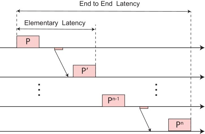
Figure 7: Latency

The elementary latency of a frame is the time duration starting from the beginning of its sending partition until the end of its last receiving partition. The end-to-end latency constrains the response time of any avionic functionality involving several communicating partitions distributed over multiple modules. For example, we might want the flight management system to display the waypoint information within $600ms$ when a pilot makes a request. We refer the reader to [7] for more detail and the formalization of the latency constraints. Let the predicate $\mathbf{LT}$ denotes the latency constraints, then the full system is formalized as follows.

$$\mathbf{AVIO}(\tilde{\varsigma}_{TT},\tilde{\gamma}_{IMA}) \stackrel{{\scriptstyle\mbox{def}}}{{=}}\;\;\mathbf{when}\;\mathbf{LT}(\tilde{\varsigma}_{TT},\tilde{\gamma}_{IMA})\;\mathbf{do}$$ (10)

$$\mathbf{IMA}(\tilde{\gamma}_{IMA})\;\|\;\mathbf{TTE}(\tilde{\varsigma}_{TT}).$$

VII Concluding Remarks

This paper presents a new simple and elegant ccp-based calculus for the analysis of real-time systems tailored for the time-triggered processes. We show the applicability of the calculus by an elegant modeling of the concepts related to the IMA and TTEthernet architectures. We also illustrate these concepts by a subsystem of the well-known flight management system.

In this exposition, however, we have considered only time-triggered traffic whilst the TTEthernet enables time-triggered and event-triggered communication, as well as integrated time-triggered/event-triggered communication on the same physical network. Our future work includes the integration of event-triggered communications as well as the study of the impact of time-triggered traffic over the latency of event-triggered traffic.

We also plan to develop a set of reasoning techniques tailored for the verification of the requirements of avionic systems. These requirements include the non-interference between any low level critical entity and a higher level critical entity. For example, the complete absence of any causal failure propagation from low level entities to high level ones. Another interesting property is the redundancy which is very common in avionic systems. We plan to develop reasoning techniques for ensuring that, from an observational point of view, a redundant system is “equivalent” to its non-redundant counterpart, for example in the absence of failures.

Finally, we plan to develop a general methodology and an associated tool for translating AADL [10] (Architecture Analysis and Design Language) and Annexes specification (e.g. [29]) into the ttcc language to allow a comprehensive analysis for avionic systems specified in this aerospace standard for model-based specification of complex real-time embedded systems.

Acknowledgments

This research is supported in part by the Collaborative Research and Development (CRD) grant No. 435325-12 jointly funded by the Consortium for Research and Innovation in Aerospace in Québec (CRIAQ) and the Natural Sciences and Engineering Research Council of Canada (NSERC) as part of project Verification of Integration of Time-Triggered Avionic Systems (VerITTAS).

References

- [1] Integrated modular avionics (ima). AERONAUTICAL RADIO, INC., ARINC 653, 2009.
- [2] Avionics full duplex switched ethernet (afdx). AERONAUTICAL RADIO, INC., ARINC 664, Part 7, 2010.
- [3] Time-triggered ethernet (ttethernet). SAE Aerospace, AS6802, 2011.
- [4] A. Al Sheikh, O. Brun, P.-E. Hladik, and B. J. Prabhu. Strictly periodic scheduling in ima-based architectures. Real-Time Systems, 48(4):359–386, 2012.
- [5] M. Alpuente, M. del Mar Gallardo, E. Pimentel, and A. Villanueva. An abstract analysis framework for synchronous concurrent languages based on source-to-source transformation. Electr. Notes Theor. Comput. Sci., 206:3–21, 2008.
- [6] R. Behjati, T. Yue, S. Nejati, L. C. Briand, and B. Selic. Extending sysml with aadl concepts for comprehensive system architecture modeling. In R. B. France, J. M. Küster, B. Bordbar, and R. F. Paige, editors, ECMFA, volume 6698 of Lecture Notes in Computer Science, pages 236–252. Springer, 2011.
- [7] S. Beji, S. Hamadou, A. Gherbi, and J. Mullins. SMT-based cost optimization approach for the integration of avionic functions in IMA and TTEthernet architectures. In The 18th IEEE/ACM International Symposium on Distributed Simulation and Real Time Applications (DS-RT’14), Toulouse, France, Oct. 2014.
- [8] P. Brémond-Grégoire, I. Lee, and R. Gerber. Acsr: An algebra of communicating shared resources with dense time and priorities. In E. Best, editor, CONCUR, volume 715 of Lecture Notes in Computer Science, pages 417–431. Springer, 1993.
- [9] F. S. de Boer, M. Gabbrielli, and M. C. Meo. A timed concurrent constraint language. Inf. Comput., 161(1):45–83, 2000.
- [10] P. H. Feiler and D. P. Gluch. Model-Based Engineering with AADL - An Introduction to the SAE Architecture Analysis and Design Language. SEI series in software engineering. Addison-Wesley, 2012.
- [11] P. V. Hentenryck, V. A. Saraswat, and Y. Deville. Design, implementation, and evaluation of the constraint language cc(fd). In A. Podelski, editor, Constraint Programming, volume 910 of Lecture Notes in Computer Science, pages 293–316. Springer, 1994.
- [12] M. Lauer. Une méthode globale pour la vérification d’exigences temps réel: application à l’Avionique Modulaire Intégrée. PhD thesis, Institut National Polytechnique de Toulouse-INPT, 2012.
- [13] J.-Y. Le Boudec and P. Thiran. Network Calculus: A Theory of Deterministic Queuing Systems for the Internet. Springer-Verlag, Berlin, Heidelberg, 2001.
- [14] A. Lescaylle and A. Villanueva. A tool for generating a symbolic representation of tccp executions. Electr. Notes Theor. Comput. Sci., 246:131–145, 2009.
- [15] X. Li, J.-L. Scharbarg, and C. Fraboul. Improving end-to-end delay upper bounds on an afdx network by integrating offsets in worst-case analysis. In ETFA, pages 1–8. IEEE, 2010.
- [16] M. Mikucionis, K. G. Larsen, J. I. Rasmussen, B. Nielsen, A. Skou, S. U. Palm, J. S. Pedersen, and P. Hougaard. Schedulability analysis using uppaal: Herschel-planck case study. In T. Margaria and B. Steffen, editors, ISoLA (2), volume 6416 of Lecture Notes in Computer Science, pages 175–190. Springer, 2010.
- [17] M. Nielsen, C. Palamidessi, and F. D. Valencia. Temporal concurrent constraint programming: Denotation, logic and applications. Nord. J. Comput., 9(1):145–188, 2002.
- [18] C. Olarte, C. Rueda, and F. D. Valencia. Models and emerging trends of concurrent constraint programming. Constraints, 18(4):535–578, 2013.
- [19] A. Philippou, I. Lee, and O. Sokolsky. Pads: An approach to modeling resource demand and supply for the formal analysis of hierarchical scheduling. Theor. Comput. Sci., 413(1):2–20, 2012.
- [20] L. T. Samarjit, L. Thiele, S. Chakraborty, and M. Naedele. Real-time calculus for scheduling hard real-time systems. In in ISCAS, pages 101–104, 2000.
- [21] D. Sangiorgi. Introduction to Bisimulation and Coinduction. Cambridge University Press, New York, NY, USA, 2011.
- [22] V. Saraswat, R. Jagadeesan, and V. Gupta. Foundations of timed concurrent constraint programming. In Proceedings, Ninth Annual IEEE Symposium on Logic in Computer Science, pages 71–80, Paris, France, 4–7 July 1994. IEEE Computer Society Press.
- [23] V. A. Saraswat. Concurrent constraint programming. ACM Doctoral dissertation awards. MIT Press, 1993.
- [24] V. A. Saraswat, R. Jagadeesan, and V. Gupta. jcc: Integrating timed default concurrent constraint programming into java. In F. Moura-Pires and S. Abreu, editors, EPIA, volume 2902 of Lecture Notes in Computer Science, pages 156–170. Springer, 2003.
- [25] V. A. Saraswat, M. C. Rinard, and P. Panangaden. Semantic foundations of concurrent constraint programming. In D. S. Wise, editor, POPL, pages 333–352. ACM Press, 1991.
- [26] G. Smolka. Concurrent constraint programming based on functional programming (extended abstract). In C. Hankin, editor, ESOP, volume 1381 of Lecture Notes in Computer Science, pages 1–11. Springer, 1998.
- [27] O. Sokolsky, I. Lee, and D. Clarke. Process-algebraic interpretation of aadl models. In F. Kordon and Y. Kermarrec, editors, Ada-Europe, volume 5570 of Lecture Notes in Computer Science, pages 222–236. Springer, 2009.
- [28] W. Steiner. An evaluation of smt-based schedule synthesis for time-triggered multi-hop networks. In Real-Time Systems Symposium (RTSS), 2010 IEEE 31st, pages 375–384. IEEE, 2010.
- [29] R. Tiyam, A. E. Kouhen, A. Gherbi, S. Hamadou, and J. Mullins, editors. Proceedings of the 1st International Architecture Centric Virtual Integration (ACVI) Workshops co-located with the ACM/IEEE 17th International Conference on Model Driven Engineering Languages and Systems (MoDELS 2014), Valencia, Spain, September 29, 2014, CEUR Workshop Proceedings. CEUR-WS.org, 2014.