Identifying the number of factors from singular values of a large sample auto-covariance matrix

Abstract

Identifying the number of factors in a high-dimensional factor model has attracted much attention in recent years and a general solution to the problem is still lacking. A promising ratio estimator based on the singular values of the lagged autocovariance matrix has been recently proposed in the literature and is shown to have a good performance under some specific assumption on the strength of the factors. Inspired by this ratio estimator and as a first main contribution, this paper proposes a complete theory of such sample singular values for both the factor part and the noise part under the large-dimensional scheme where the dimension and the sample size proportionally grow to infinity. In particular, we provide the exact description of the phase transition phenomenon that determines whether a factor is strong enough to be detected with the observed sample singular values. Based on these findings and as a second main contribution of the paper, we propose a new estimator of the number of factors which is strongly consistent for the detection of all significant factors (which are the only theoretically detectable ones). In particular, factors are assumed to have the minimum strength above the phase transition boundary which is of the order of a constant; they are thus not required to grow to infinity together with the dimension (as assumed in most of the existing papers on high-dimensional factor models). Empirical Monte-Carlo study as well as the analysis of stock returns data attest a very good performance of the proposed estimator. In all the tested cases, the new estimator largely outperforms the existing estimator using the same ratios of singular values.

http://arxiv.org/abs/1410.3687

and and

1 Introduction

Factor models have met a large success in data analysis in many scientific fields such as psychology, economics and finance, signal processing, to name a few. One of the strengths of these models relies on its capability to reduce the generally high dimension of the data to a much lower-dimensional common component. The structure of these models is complex and many different versions of the models have been introduced so far in the long-standing literature on the subject, ranging from static to dynamic or generalized dynamic factor models on one hand, and from exact to approximate factor models on the other hand. A recent survey of this literature can be found in Stock and Watson [25]. Efforts are however still paid to the study of these models because unfortunately their inference is not easy, especially when the cross-sectional dimension $p$ and the temporal dimension $T$ are both large.

In such high-dimensional context, the determination of the number $k$ of common factors in in a factor model is a challenging problem. Misspecification of this number can deeply affect the quality of the fitted factor model. In this context, the seminal paper Bai and Ng [2] provided for the first time a consistent estimator of $k$ for static factor models. This estimator has attracted much attention afterwards, and has been improved or generalized, e.g. in Bai and Ng [3] by the authors themselves, in Hallin and Liska [14] for dynamic factor models and in Alessi et al. [1] for approximate factor models. It should be here mentioned that as these developments mainly target at analysis of economic or financial data, the common factors in these models are thought to be pervasive, or strong, in the sense that their strength is much higher than the strength of the idiosyncratic (error) component. The asymptotic consistency of the factor number estimator depends in a large extent on this assumption. However, some recent studies on factor models suggest the importance for accommodating more factors in these models by including some weaker factors which still have a significant explanation power on both cross-sectional and temporal correlations of the data. For example, Onatski [22] makes a clear distinction between strong factors and weak factors when considering asymptotic approximations of the square loss function from a principal components-based perspective. A related work allowing weak factors can be found in Onatski [21].

In this paper we consider a factor model for high-dimensional time series proposed by Lam and Yao [17]: the observations $Y$ is a $p\times T$ matrix with $p$ cross-sectional units over $T$ time periods. Let $y_{t}$ denote the $p$-dimensional vector observed at time $t$, then it consists of two components, a low dimensional common-factor time series $x_{t}$ and an idiosyncratic component $\varepsilon_{t}$:

$$y_{t}=Ax_{t}+\varepsilon_{t},$$ (1.1)

where $A$ is the factor loading matrix of size $p\times k$ and $\{\varepsilon_{t}\}$ is a white noise sequence (temporal uncorrelated). The factors in $(x_{t})$ are here loaded contemporaneously; however this is a time series and its temporal correlation implies that of the observations $\{y_{t}\}$. However, this is the unique source of temporal correlation, and in this aspect, the model is much more restrictive than the general dynamic models as introduced in Geweke [13], Sargent and Sims [24] and Forni et al. [10, 11, 12]. Nevertheless, there are two advantages in this simplified model. First, since potentially $(x_{t})$ can be any kind of stationary time series of low dimension, the model can already cover a wide range of applications. Second, inference procedures are here more consistently defined and more precise results can be expected, e.g. for the determination of the number of factors. The factor model (1.1) can be considered as a good balance between the generality of model coverage and the technical feasibility of underlying inference procedures.

The goal of this paper is to develop a powerful estimator of the number of factors in the model (1.1). Lam and Yao [17] proposed a ratio-based estimator defined as follows. Let $\Sigma_{y}{}=\mathop{\text{cov}}(y_{t},y_{t-1})$ and $\Sigma_{x}{}=\mathop{\text{cov}}(x_{t},x_{t-1})$ be the lag-1 auto-covariance matrices of $y_{t}$ and $x_{t}$, respectively. Assuming that the factor and the noise are independent, we then have

$$\Sigma_{y}{}=A\Sigma_{x}{}A^{\prime}\leavevmode\nobreak\ ,$$

which leads to its symmetric counterpart

$$M=\Sigma_{y}{}\Sigma_{y}{}^{\prime}=A\Sigma_{x}{}\Sigma_{x}{}^{\prime}A^{\prime}\leavevmode\nobreak\ .$$ (1.2)

Since in general the $k\times k$ matrix $\Sigma_{x}{}$ is of full rank $k$, the symmetric $p\times p$ matrix $M$ has exactly $k$ nonzero eigenvalues. Moreover, the factor loading space $\mathcal{M}(A)$, i.e. the $k$-dimensional subspace in $\mathbb{R}^{p}$ generated by the columns of $A$, is spanned by the eigenvectors of $M$ corresponding to its nonzero eigenvalues $a_{1}\geq\cdots\geq a_{k}>0$ (factor eigenvalues). Let

$$\widehat{M}=\widehat{\Sigma}_{y}{}\widehat{\Sigma}_{y}{}^{\prime},\quad\text{where}\leavevmode\nobreak\ \widehat{\Sigma}_{y}{}=\frac{1}{T}\sum_{t=2}^{T+1}y_{t}y_{t-1}^{\prime}\leavevmode\nobreak\ ,$$ (1.3)

be the sample counterparts of $M$ and $\Sigma_{y}{}$, respectively. The main observation is that the $p-k$ null eigenvalues of $M$ will lead to $p-k$ “relatively small” sample eigenvalues in $\widehat{M}$, while the $k$ factor eigenvalues $(a_{i})$ will generate $k$ “relatively large” eigenvalues in $\widehat{M}$. This can be made very precisely in a classical low-dimensional framework where we fix the dimension $p$ and let $T$ grow to infinity: indeed by law of large numbers, $\widehat{M}\to M$ and by continuity, all the eigenvalues $l_{1}\geq l_{2}\geq\cdots\geq l_{p}$ (sorted in decreasing order) of $\widehat{M}$ will converge to the corresponding eigenvalues of $M$. In particular, for $k<i\leq p$, $l_{i}\to 0$ while $l_{i}\to a_{i}>0$ for $1\leq i\leq k$. Consider the ratio estimator (Lam and Yao [17]):

$$\tilde{k}=\arg\min_{1\leq i<p}{l_{i+1}}/{l_{i}}.$$ (1.4)

As $l_{k+1}/l_{k}$ will be the first ratio in this list which tends to zero, $\tilde{k}$ will be a consistent estimator of $k$.

In the high-dimensional context however, $\widehat{M}$ will significantly deviate from $M$ and the spectrum $(l_{i})$ of $\widehat{M}$ will not be close to that of $M$ anymore. In particular, the time for the first minimum of the ratios in (1.4) becomes noisy and can be much different from the target value $k$. Notice that the $k$ non-null factor eigenvalues $(a_{i})$ are directly linked to the strength of the factor time series $(x_{t})$. The precise relationship between the ratios of sample eigenvalues in (1.4) will ultimately depend on a complex interplay between the strength of the factor eigenvalues $(a_{i})$ (compared to the noise level), the dimension $p$ and the sample size $T$.

Despite of the introduction of a very appealing ratio estimator (1.4), precise description of the sample ratios ${l_{i+1}}/{l_{i}}$ is missing in [17]. Indeed, the authors establish the consistency of the ratio estimator $\tilde{k}$ by requiring that the factor strengths $(a_{i})$ all explode at a same rate: $a_{i}\propto p^{\delta}$ for all $1\leq i\leq k$ and some $\delta>0$ as the dimension $p$ grows to infinity. In other words, the factors are all strong and they have a same asymptotic strength. This limitation is quite severe because factors with different levels of strength cannot be all detected within this framework. For instance, if we have factors with say three levels of strength $p^{\delta_{j}}$, $j=1,2,3$ where $\delta_{1}>\delta_{2}>\delta_{3}$, the ratio estimator $\tilde{k}$ above will correctly identify the group of strongest factors $a_{i}\propto p^{\delta_{1}}$ while all the others will be omitted. In an attempt to correct such undesirable behavior, a two-step estimation procedure is also proposed in [17] which will identify successively two groups of factors with top two strengths: this means that in the example above, factors of strength $a_{i}$’ proportional to $p^{\delta_{j}}$ with $j=1,2$ will be identified while the others will remain omitted. The issue here is that a priori, we do not know how many different levels of strength the factors could have and it is unlikely we could attempt to estimate such different levels as this would lead to a problem that is equally (if not more) difficult than the initial problem of estimating the number of factors.

Inspired by the appropriateness of the ratio estimator $\tilde{k}$ in the high-dimensional context, the main objective of this paper is to provide a rigorous theory for the estimation of the number of factors based on the ratios $\{l_{i+1}/l_{i}\}$ under the high-dimensional setting where $p$ and $T$ tend to infinity proportionally.

The paper contains two main contributions. First, we characterize completely the limits of both the factor eigenvalues $\{l_{i}\}_{1\leq i\leq k}$ and the noise eigenvalues $\{l_{i}\}_{k<i\leq p}$. For the noise part, as $k$ (although unknown) is much smaller than the dimension $p$, we prove that the spectral distribution generated by $\{l_{i}\}_{k<i\leq p}$ has a limit which coincide with the limit of the spectral distribution generated by the $p$ eigenvalues of the (unobserved) matrix $\widehat{M}_{\varepsilon}=\widehat{\Sigma}_{\varepsilon}\widehat{\Sigma}^{\prime}_{\varepsilon}$ where $\Sigma_{\varepsilon}=T^{-1}\sum_{t=2}^{T+1}\varepsilon_{t}\varepsilon^{\prime}_{t-1}$. This limiting distribution has been explored elsewhere in Li et al. [1] and its support found to be a compact interval $[a,b]$. As for the factor part $\{l_{i}\}_{1\leq i\leq k}$, although it is highly expected that they should have a limit located outside the base interval $[a,b]$, we establish a phase transition phenomenon: a factor eigenvalue $l_{i}$ will tend to a limit $\lambda_{i}>b$ (outlier) if and only if the corresponding population factor strength $a_{i}$ exceeds some critical value $\tau$. In other words, if a factor $a_{i}$ is too weak, then the corresponding sample factor eigenvalue $\lambda_{i}$ will tend to $b$, the (limit of) maximum of the noise eigenvalues and it will be hardly detectable. Moreover, both the outlier limits $\{\lambda_{i}\}$ and the critical value $\tau$ are characterized through the model parameters.

The second main contribution of the paper is the derivation of a new estimator $\widehat{k}$ of the number of factors based on the finding above. If $k_{0}$ denotes the number of significant factors, i.e. with factor strength $a_{i}>\tau$, then using an appropriate thresholding interval $(1-d_{T},1)$ for the sample ratios $\{l_{i+1}/l_{i}\}$, the derived estimator $\widehat{k}$ is strongly consistent converging to $k_{0}$. In addition to this well-justified consistency, the main advantage of the proposed estimator is its robustness against possibly multiple levels of factor strength; in theory, all factors with strength above the constant $\tau$ are detectable. Therefore, both strong factors and weak factors can be present, and their strengths can have different asymptotic rates with regard to the dimension $p$ in order to be detected from the observed samples. This is a key difference between the method provided in this paper and most of existing estimators of the factor number as recalled previously (the reader is however reminded that the model (1.1) is more restrictive than a general dynamic factor model). Notice however that these precise results have been obtained at the cost of some drastic simplification of the idiosyncratic component $\{\varepsilon_{t}\}$, namely independence has been assumed both serially and cross-sectionally (over the time and the dimension), and the components are normalized to have a same value of variance (see Assumption 2 in Section 2). These limitations are required by the technical tools employed in this paper and some non-trivial extension of these tools are needed to get rid of these limitations.

From a methodological point of view, our approach is based on recent advances from random matrix theory, specifically on the so-called spiked population models or more generally on finite-rank perturbations of large random matrices. We start by identifying the sample matrix $\widehat{M}$ as a finite-rank perturbation of the base matrix $\widehat{M}_{\varepsilon}$ associated to the noise. In a recent paper Li et al. [1], the limiting spectral distribution of the eigenvalues of $\widehat{M}_{\varepsilon}$ has been found and the base interval $[a,b]$ characterized. By developing the mentioned perturbation theory for the autocovariance matrix $\widehat{M}$, we find the characterization of the limits of its eigenvalues $\{l_{i}\}$.

For the strong consistency of the proposed ratio estimator $\widehat{k}$, a main ingredient is the almost sure convergence of the largest eigenvalue of the base matrix $\widehat{M}_{\varepsilon}$ to the right edge $b$, recently established in Wang and Yao [27]. This result serves as the cornerstone for distinguishing between significant factors and noise components.

It is worth mentioning a related paper Onatski [20] where the author stands from a similar perspective with the method in this paper. However, that paper addresses static approximate factor models without time series dependence and more importantly, the assumption of explosion of all factor eigenvalues is still required which, on the contrary, is released in this paper. Other related references include Jin et al. [15] and Wang et al. [26] where the limiting spectral distribution and the strong convergence of extreme eigenvalues are derived for the matrix $\frac{1}{2}({\widehat{\Sigma}}_{\varepsilon}+{\widehat{\Sigma}}^{\prime}_{\varepsilon})$. One should mention that these works are more related to the study in Li et al. [1] and Wang and Yao [27] on spectral limits of the matrix ${\widehat{M}}_{\varepsilon}$, and they have no results either on convergence of the spiked (factor) eigenvalues or on the estimation of the number of factors as proposed in this paper.

The rest of the paper is organized as follows. In Section 2, after introduction of the model assumptions we develop our first main result regarding spectral limits of $\widehat{M}$. The new estimator $\widehat{k}$ is then introduced in Section 3 and its strong convergence to the number of significant factors $k_{0}$ established. In Section 4, detailed Monte-Carlo experiments are conducted to check the finite-sample properties of the proposed estimator and to compare it with the ratio estimator $\tilde{k}$ (1.4) from Lam and Yao [17]. Both estimators $\tilde{k}$ and $\widehat{k}$ are next tested in Section 5 on a real data set from Standard & Poor stock returns and compared in details. Notice that some technical lemmas used in the main proofs are gathered in a companion paper of supplementary material Li et al. [19].

2 Large-dimensional limits of noise and factor eigenvalues

The static factor model (1.1) is further specified to satisfy the following assumptions.

Assumption 1. The factor $(x_{t})$ is a $k$-dimensional ($k\ll p$ fixed) stationary time series, each dimension is independent of each other, with the representation of each component:

$$x_{it}=\sum_{l=0}^{\infty}\phi_{il}\eta_{i\,t-l}\leavevmode\nobreak\ ,i=1,\cdots,k,\leavevmode\nobreak\ t=1,\cdots,T,$$

where $(\eta_{ik})$ is a real-valued and weakly stationary white noise with mean 0 and variance $\sigma_{i}^{2}$. The series $\{x_{it}\}$ has variance $\gamma_{0}(i)$ and lag-1 auto-covariance $\gamma_{1}(i)$. Moreover, the variance $\gamma_{0}(i)$ will be hereafter referred as the strength of the $i$-th factor time series $\{x_{it}\}$.

Assumption 2. The idiosyncratic component $(\varepsilon_{t})$ is independent of $x_{t}$. $\varepsilon_{t}$ is $p-$dimensional real valued random vector with independent entries $\varepsilon_{it},\leavevmode\nobreak\ i=1,\cdots,p$, not necessarily identically distributed, satisfying

$$\mathbb{E}(\varepsilon_{i\,t})=0,\leavevmode\nobreak\ \mathbb{E}(\varepsilon_{i\,t}^{2})=\sigma^{2},$$

and for any $\eta>0$,

$$\frac{1}{\eta^{4}pT}\sum_{i=1}^{p}\sum_{t=1}^{T+1}\mathbb{E}\left(|\varepsilon_{i\,t}|^{4}I_{(|\varepsilon_{i\,t}|\geq\eta T^{1/4})}\right)\longrightarrow 0\quad\text{as }(pT)\to\infty.$$ (2.1)

Assumption 3. The dimension $p$ and the sample size $T$ tend to infinity proportionally: $p\to\infty$, $T=T(p)\to\infty$ and $p/T\rightarrow y>0$.

Assumption 1 defines the static factor model considered in this paper. Assumption 2 details the moment condition and the independent structure of the noise. In particular, (2.1) is a Lindeberg-type condition widely used in random matrix theory. In particular, if the fourth moments of the variables $\{\varepsilon_{it}\}$ are uniformly bounded, the Lindeberg condition is satisfied. Assumption 3 defines the high-dimensional setting where the dimension and the sample size can be both large without however one dominating the other.

First we have,

$$\widehat{\Sigma}_{y}{} =\frac{1}{T}\sum_{t=2}^{T+1}y_{t}y_{t-1}^{\prime}=\frac{1}{T}\sum_{t=2}^{T+1}(Ax_{t}+\varepsilon_{t})(Ax_{t-1}+\varepsilon_{t-1})^{\prime}$$

$$=\frac{1}{T}\sum_{t=2}^{T+1}Ax_{t}x_{t-1}^{\prime}A^{\prime}+\frac{1}{T}\sum_{t=2}^{T+1}\left(Ax_{t}\varepsilon_{t-1}^{\prime}+\varepsilon_{t}x_{t-1}^{\prime}A^{\prime}\right)+\frac{1}{T}\sum_{t=2}^{T+1}\varepsilon_{t}\varepsilon_{t-1}^{\prime}$$

$$:={P}_{A}+\widehat{\Sigma}_{\varepsilon}{}.$$

The matrix $\widehat{\Sigma}_{\varepsilon}{}=T^{-1}\sum_{t}\varepsilon_{t}\varepsilon_{t-1}^{\prime}$ is the analogous sample autocovariance matrix associated to the noise $(\varepsilon_{t})$. Since $A$ has rank $k$, the rank of the matrix $P_{A}$ is bounded by $2k$ (we will see in fact that asymptotically, the rank of $P_{A}$ will be eventually $k$). Therefore, the autocovariance matrix of interest $\widehat{\Sigma}_{y}{}$ is seen as a finite-rank perturbation of the noise autocovariance matrix $\widehat{\Sigma}_{\varepsilon}{}$. Since the matrix $\widehat{\Sigma}_{y}{}$ is not symmetric, we consider its singular values, which are also the square root of the eigenvalues of $\widehat{M}:=\widehat{\Sigma}_{y}{}\widehat{\Sigma}^{{}^{\prime}}_{y}{}$. Therefore, the study of the singular values of $\widehat{\Sigma}_{y}{}$ reduces to the study of the eigenvalues of $\widehat{M}$, which is also a finite rank perturbation of the base component $\widehat{M}_{\varepsilon}:=\widehat{\Sigma}_{\varepsilon}{}\widehat{\Sigma}^{{}^{\prime}}_{\varepsilon}$.

Finite-rank perturbations of random matrices have been actively studied in recent years and the theory is much linked to the spiked population models well known in high-dimensional statistics literature. For some recent accounts on this theory, we refer to Johnstone [16], Baik and Silverstein [7], Bai and Yao [5], Benaych-Georges and Nadakuditi [8], Passemier and Yao [23] and the references therein. A general picture from this theory is that first, the eigenvalues of the base matrix will converge to a limiting spectral distribution (LSD) with a compact support, say an interval $[a,b]$; and secondly, for the eigenvalues of the perturbed matrices, most of them (base eigenvalues) will converge to the same LSD independently of the perturbation while a small number among the largest ones will converge to a limit outside the support of the LSD (outliers). However, all the existing literature cited above concern the finite rank perturbation of large-dimensional sample covariance matrices or Wigner matrices. As a theoretic contribution of the paper, we extend this theory to the case of a perturbed auto-covariance matrix by giving exact conditions under which the aforementioned dichotomy between base eigenvalues and outliers still hold. Specifically, it will be proved in this section that once the $k$ factor strengths $(a_{i})$ are not “too weak”, they will generate exactly $k$ outliers, while the remaining $p-k$ eigenvalues will behave as the eigenvalues of the base $\widehat{M}_{\varepsilon}$, which converges to a compactly supported LSD.

It is then apparent that under such dichotomy and by “counting” the outliers outside the interval $[a,b]$, we will be able to obtain a consistent estimator of the number of factors $k$.

In what follows, we first recall two existing result on the asymptotic of the singular values of $\widehat{\Sigma}_{\varepsilon}{}$. Then we develop our theory on the limits of largest (outliers) and base singular values of $\widehat{\Sigma}_{y}{}$.

2.1 Limiting spectral distribution of $\widehat{M}_{\varepsilon}{}$

We first recall two useful results on the base matrix $\widehat{M}_{\varepsilon}{}$. Firstly, the limiting spectral distribution of the eigenvalues of $\widehat{M}_{\varepsilon}{}$ has been obtained in a recent paper Li et al. [1]. Write

$$\widehat{M}_{\varepsilon} =\left(\frac{1}{T}\sum_{t=2}^{T+1}\varepsilon_{t}\varepsilon_{t-1}^{\prime}\right)\left(\frac{1}{T}\sum_{t=2}^{T+1}\varepsilon_{t}\varepsilon_{t-1}^{\prime}\right)^{\prime}$$

$$=\frac{1}{T^{2}}XY^{\prime}YX^{\prime}\leavevmode\nobreak\ ,$$

with the data matrices

$$X=\left(\begin{array}[]{ccc}\varepsilon_{12}&\cdots&\varepsilon_{1,T+1}\\ \vdots&\ddots&\vdots\\ \varepsilon_{p2}&\cdots&\varepsilon_{p,T+1}\end{array}\right),\quad Y=\left(\begin{array}[]{ccc}\varepsilon_{11}&\cdots&\varepsilon_{1T}\\ \vdots&\ddots&\vdots\\ \varepsilon_{p1}&\cdots&\varepsilon_{pT}\end{array}\right).$$

Furthermore, let $\mu$ be a measure on the real line supported on an interval $[\alpha,\beta]$ (the end points can be infinity), with its Stieltjes transform defined as

$$m(z)=\int\frac{1}{t-z}d\mu(t)\leavevmode\nobreak\ \quad\mbox{for}\leavevmode\nobreak\ z\in\mathbb{C}\backslash\text{supp}(\mu)\leavevmode\nobreak\ ,$$

and its $T$-transform as

$$T(z)=\int\frac{t}{z-t}d\mu(t)\leavevmode\nobreak\ \quad\mbox{for}\leavevmode\nobreak\ z\in\mathbb{C}\backslash\text{supp}(\mu).$$

Notice here that the T-transform is a decreasing homeomorphism from $(-\infty,\alpha)$ onto $(T(\alpha^{-}),0)$ and from $(\beta,+\infty)$ onto $(0,T(\beta^{+}))$, which related to each other by the following equation:

$$T(z)=-1-zm(z)\leavevmode\nobreak\ .$$

Proposition 2.1.

[Li et al. [1]]

Suppose that Assumptions 2 and 3 hold with $\sigma^{2}=1$. Then, the empirical spectral distribution of $B:=1/T^{2}Y^{\prime}YX^{\prime}X$ ( which is the companion matrix of $\widehat{M}_{\varepsilon}$) converges a.s. to a non-random limit F, whose Stieltjes transform $m=m(z)$ satisfies the equation

$$z^{2}m^{3}(z)-2z(y-1)m^{2}(z)+(y-1)^{2}m(z)-zm(z)-1=0\leavevmode\nobreak\ .$$ (2.2)

In particular, this LSD is supported on the interval $[a\mathbf{1}_{\{y\geq 1\}},b]$ whose end points are

$$a=\left(-1+20y+8y^{2}-(1+8y)^{3/2}\right)/8\leavevmode\nobreak\ ,$$ (2.3)

$$b=\left(-1+20y+8y^{2}+(1+8y)^{3/2}\right)/8\leavevmode\nobreak\ .$$ (2.4)

Notice that the companion matrix $B$ is $T\times T$ and it shares the same $p\wedge T$ non-null eigenvalues as $\widehat{M}_{\varepsilon}$, therefore, the support of $\widehat{M}_{\varepsilon}$ is also $[a,b]$ The LSD $F$ of $B$ and the LSD $F^{*}$ of $\widehat{M}_{\varepsilon}$ are linked by the relationship

$$yF^{*}-F=(y-1)\delta_{0}\leavevmode\nobreak\ ,$$

where $\delta_{0}$ is the Dirac mass at the origin.

Remark 2.1.

The equation (2.2) can be expressed using the $T$-transform:

$$\left(T(z)+1\right)\left(T(z)+y\right)^{2}=zT(z)$$ (2.5)

The second result is about the convergence of the largest eigenvalue of $\widehat{M}_{\varepsilon}$.

Proposition 2.2.

[Wang and Yao [27]]

Suppose that Assumptions 2 and 3 hold with $\sigma^{2}=1$. Then, the largest eigenvalue of $\widehat{M}_{\varepsilon}$ converges a.s. to the right end point $b$ of its LSD given in (2.4).

Combining Propositions 2.1 and 2.2, we have the following corollary.

Corollary 2.1.

Under the same conditions as in Proposition 2.2, if $(\beta_{j})$ are sorted eigenvalues of $\widehat{M}_{\varepsilon}$, then for any fixed $m$, the $m$ largest eigenvalues $\beta_{1}\geq\beta_{2}\geq\cdots\geq\beta_{m}$ all converge to $b$.

Proof.

For any $\delta>0$, almost surely the number of sample eigenvalues of $\beta_{j}$ falling into the interval $(b-\delta,b)$ grows to infinity due to the fact the density of the LSD is positive and continuous on this interval. Then for fixed $m$, a.s. $\liminf_{p\to\infty}\beta_{m}\geq b-\delta$. By letting $\delta\to 0$, we have a.s. $\liminf_{p\to\infty}\beta_{m}\geq b$. Obviously, $\limsup_{p\to\infty}\beta_{m}\leq\limsup_{p\to\infty}\beta_{1}=b$, i.e a.s. $\lim_{p\to\infty}\beta_{m}=b$. ∎

2.2 Convergence of the largest eigenvalues of the sample autocovariance matrix $\widehat{M}$

The following main result of the section characterizes the limits of the $k$-largest eigenvalues of the sample autocovariance matrix $\widehat{M}$.

Theorem 2.1.

Suppose that the model (1.1) satisfies Assumptions 1, 2 and 3 and that the noise $\{\varepsilon_{t}\}$ are normal distributed and the loading matrix $A$ is normalized as $A^{\prime}A=I_{k}$. Let $l_{i}\leavevmode\nobreak\ (1\leq i\leq k)$ denote the $k$ largest eigenvalue of $\widehat{M}$. Then for each $1\leq i\leq k$, $l_{i}/\sigma^{4}$ converges almost surely to a limit $\lambda_{i}$. Moreover,

$$\lambda_{i}=b\quad\text{when}\leavevmode\nobreak\ \leavevmode\nobreak\ T_{1}(i)\geq T(b^{+}),$$

where

$$T_{1}(i)=\frac{2y\sigma^{2}\gamma_{0}(i)+\gamma_{1}(i)^{2}-\sqrt{(2y\sigma^{2}\gamma_{0}(i)+\gamma_{1}(i)^{2})^{2}-4y^{2}\sigma^{4}(\gamma_{0}(i)^{2}-\gamma_{1}(i)^{2})}}{2\gamma_{0}(i)^{2}-2\gamma_{1}(i)^{2}}\leavevmode\nobreak\ .$$ (2.6)

Otherwise, i.e. $T_{1}(i)<T(b^{+})$, $\lambda_{i}>b$ and its value is characterized by the fact that the $T$-transform $T(\lambda_{i})$ is the solution to the equation:

$$\left(y\sigma^{2}-\gamma_{0}(i)T(\lambda_{i})\right)^{2}=\gamma_{1}(i)^{2}T(\lambda_{i})\left(1+T(\lambda_{i})\right)\leavevmode\nobreak\ .$$ (2.7)

The theorem establishes a phase transition phenomenon for the $k$ sample factor eigenvalues $(l_{i})$. Define the number of significant factors

$$k_{0}=\sharp\left\{1\leq i\leq k:\leavevmode\nobreak\ T_{1}(i)<T(b^{+})\right\}.$$ (2.8)

Therefore, for each of the $k_{0}$ significant factor, the corresponding sample eigenvalue $l_{i}$ will converge to a limit $\lambda_{i}$ outside the base support interval $[a,b]$. In contrary, for the $k-k_{0}$ factors for which $T_{1}(i)\geq T(b^{+})$, they are too weak in the sense that the corresponding sample eigenvalue $l_{i}$ will converge to $b$ which is also the limit of the largest noise eigenvalues $l_{k+1},\ldots,l_{k+m}$ ($m$ is a fixed number here). Therefore, these weakest factors will be merged with noise component and their detection becomes hardly possible.

Later in Section 2.3, it will be established that for the $i$-th factor time series be significant, the phase transition condition $T_{1}(i)<T(b^{+})$ essentially requires the strength $\gamma_{0}(i)$ be large enough.

Proof.

(of Theorem 2.1) The proof consists in four steps where some technical lemmas are to be found in the companion paper of supplementary material Li et al. [19].

Step 1. Simplification of variance $\sigma^{2}$ of white noise $\{\varepsilon_{i\,t}\}$. To ease the complexity of the proof of this main theorem, we firstly reduce the variance of the white noise from $\sigma^{2}$ to 1. In our model setting, we have (1.1) equivalent to

$$\frac{y_{t}}{\sigma}=A\frac{x_{t}}{\sigma}+\frac{\varepsilon_{t}}{\sigma}\leavevmode\nobreak\ .$$

And if we denote $\tilde{y}_{t}=y_{t}/\sigma$, $\tilde{x}_{t}=x_{t}/\sigma$ and $\tilde{\varepsilon}_{t}=\varepsilon_{t}/\sigma$, then we are dealing with the model

$$\tilde{y}_{t}=A\tilde{x}_{t}+\tilde{\varepsilon}_{t}\leavevmode\nobreak\ ,$$ (2.9)

where the white noise $\tilde{\varepsilon}$ has mean zero and unit variance and the variance and autocovariance of the factor process $\{\tilde{x}_{t}\}$ satisfies

$$\tilde{\gamma}_{0}(i)=\gamma_{0}(i)/\sigma^{2}\leavevmode\nobreak\ ,\tilde{\gamma}_{1}(i)=\gamma_{1}(i)/\sigma^{2}\leavevmode\nobreak\ ,$$ (2.10)

in which $\gamma_{0}(i)$ and $\gamma_{1}(i)$ are the variance and autocovariance of the original factor process $\{x_{t}\}$. Therefore, in all the following, we just consider the standardized Model (2.9). For convenience, we use notations of the original model (1.1) and set $\sigma^{2}=1$ to investigate Model (2.9). At the end of the proof, we will replace the value of $\gamma_{0}(i)$ and $\gamma_{1}(i)$ with $\tilde{\gamma}_{0}(i)$ and $\tilde{\gamma}_{1}(i)$ to recover the corresponding results for Model (1.1).

Step 2. Simplification of matrix $A$. Here we argue that it is enough to consider the case where the loading matrix $A$ has the canonical form

$$A=\begin{pmatrix}I_{k}\\ \bm{0}_{p-k}\\ \end{pmatrix}\leavevmode\nobreak\ .$$

Indeed, suppose $A$ is not in this canonical form. Since by assumption $A^{\prime}A=I_{k}$, we can complete $A$ to an orthogonal matrix $Q=(A,C)$ by adding appropriate orthonormal columns. From the model equation (1.1), we have

$$Q^{\prime}y_{t}=Q^{\prime}Ax_{t}+Q^{\prime}\varepsilon_{t}=\begin{pmatrix}A^{\prime}\\ C^{\prime}\\ \end{pmatrix}Ax_{t}+Q^{\prime}\varepsilon_{t}=\begin{pmatrix}I_{k}\\ \bm{0}_{p-k}\\ \end{pmatrix}x_{t}+Q^{\prime}\varepsilon_{t}\leavevmode\nobreak\ .$$

Since $\varepsilon_{t}\sim\mathcal{N}(0,I_{p})$ and $Q^{\prime}$ is orthogonal, $Q^{\prime}\varepsilon_{t}\sim\mathcal{N}(0,I_{p})$. Let $z_{t}:=Q^{\prime}y_{t}$, then $z_{t}$ satisfies the model equation (1.1) with a canonical loading matrix. What happens is that the singular values of the two lag-1 autocovariance matrices

$$\frac{1}{T}\sum_{t=2}^{T+1}z_{t}z_{t-1}^{\prime},\quad\frac{1}{T}\sum_{t=2}^{T+1}y_{t}y_{t-1}^{\prime}$$

are the same: this is simply due to fact that

$$\leavevmode\nobreak\ \leavevmode\nobreak\ \leavevmode\nobreak\ \leavevmode\nobreak\ \left(\frac{1}{T}\sum_{t=2}^{T+1}y_{t}y_{t-1}^{\prime}\right)\left(\frac{1}{T}\sum_{t=2}^{T+1}y_{t}y_{t-1}^{\prime}\right)^{\prime}$$

$$=\left(\frac{1}{T}\sum_{t=2}^{T+1}Q^{\prime}z_{t}\cdot(Q^{\prime}z_{t-1})^{\prime}\right)\left(\frac{1}{T}\sum_{t=2}^{T+1}Q^{\prime}z_{t}\cdot(Q^{\prime}z_{t-1})^{\prime}\right)^{\prime}$$

$$=Q^{\prime}\left(\frac{1}{T}\sum_{t=2}^{T+1}z_{t}z_{t-1}^{\prime}\right)\left(\frac{1}{T}\sum_{t=2}^{T+1}z_{t}z_{t-1}^{\prime}\right)^{\prime}Q\leavevmode\nobreak\ .$$

Step 3. Derivation of the main equation (2.7) From now on we assume that $A$ is in its canonical form. By the definition of $y_{t}$, we have

$$\leavevmode\nobreak\ \leavevmode\nobreak\ \leavevmode\nobreak\ \leavevmode\nobreak\ \widehat{\Sigma}_{y}{}=\frac{1}{T}\sum_{t=2}^{T+1}y_{t}y_{t-1}^{\prime}$$

$$=\frac{1}{T}\sum_{t=2}^{T+1}\begin{pmatrix}x_{1\,t}+\varepsilon_{1\,t}\\ \vdots\\ x_{k\,t}+\varepsilon_{k\,t}\\ \varepsilon_{k+1\,t}\\ \vdots\\ \varepsilon_{p\,t}\\ \end{pmatrix}\begin{pmatrix}x_{1\,t-1}+\varepsilon_{1\,t-1}&\cdots&x_{k\,t-1}+\varepsilon_{k\,t-1}&\varepsilon_{k+1\,t-1}&\cdots&\varepsilon_{p\,t-1}\\ \end{pmatrix}$$

$$:=\begin{pmatrix}A&B\\ C&D\\ \end{pmatrix}\leavevmode\nobreak\ ,$$ (2.11)

where we use $A$, $B$, $C$ and $D$ to denote the four blocks. Besides, if we use the notation:

$$X_{0}:=\frac{1}{\sqrt{T}}\begin{pmatrix}x_{1\,1}+\varepsilon_{1\,1}&\cdots&x_{k\,1}+\varepsilon_{k\,1}\\ \vdots&\ddots&\vdots\\ x_{1\,T}+\varepsilon_{1\,T}&\cdots&x_{k\,T}+\varepsilon_{k\,T}\\ \end{pmatrix}\leavevmode\nobreak\ ,$$

$$X_{1}:=\frac{1}{\sqrt{T}}\begin{pmatrix}x_{1\,2}+\varepsilon_{1\,2}&\cdots&x_{k\,2}+\varepsilon_{k\,2}\\ \vdots&\ddots&\vdots\\ x_{1\,T+1}+\varepsilon_{1\,T+1}&\cdots&x_{k\,T+1}+\varepsilon_{k\,T+1}\\ \end{pmatrix}\leavevmode\nobreak\ ,$$

$$E_{1}:=\frac{1}{\sqrt{T}}\begin{pmatrix}\varepsilon_{k+1\,1}&\cdots&\varepsilon_{p\,1}\\ \vdots&\ddots&\vdots\\ \varepsilon_{k+1\,T}&\cdots&\varepsilon_{p\,T}\\ \end{pmatrix},\leavevmode\nobreak\ \leavevmode\nobreak\ \quad E_{2}:=\frac{1}{\sqrt{T}}\begin{pmatrix}\varepsilon_{k+1\,2}&\cdots&\varepsilon_{p\,2}\\ \vdots&\ddots&\vdots\\ \varepsilon_{k+1\leavevmode\nobreak\ T+1}&\cdots&\varepsilon_{p\leavevmode\nobreak\ T+1}\\ \end{pmatrix}\leavevmode\nobreak\ ,$$

then we have

$$A=X_{1}^{\prime}X_{0}\leavevmode\nobreak\ ,\leavevmode\nobreak\ \leavevmode\nobreak\ B=X_{1}^{\prime}E_{1}\leavevmode\nobreak\ ,\leavevmode\nobreak\ \leavevmode\nobreak\ C=E_{2}^{\prime}X_{0}\leavevmode\nobreak\ ,\leavevmode\nobreak\ \leavevmode\nobreak\ D=E_{2}^{\prime}E_{1}\leavevmode\nobreak\ .$$ (2.12)

Since $l$ is the extreme large eigenvalue of $\widehat{\Sigma}_{y}{}\widehat{\Sigma}_{y}{}^{\prime}$, $\sqrt{l}$ is the extreme large singular value of $\widehat{\Sigma}_{y}{}$, which is also equivalent to saying that $\sqrt{l}$ is the positive eigenvalue of the $2p\times 2p$ matrix

$$\left(\begin{array}[]{cc}0&\widehat{\Sigma}_{y}{}\\ \widehat{\Sigma}_{y}{}^{\prime}&0\\ \end{array}\right)\leavevmode\nobreak\ .$$ (2.13)

And use the block expression (2.11), combining with the definition of each block in (2.12), (2.13) is equivalent to

$$\left(\begin{array}[]{cccc}0&0&X_{1}^{\prime}X_{0}&X_{1}^{\prime}E_{1}\\ 0&0&E_{2}^{\prime}X_{0}&E_{2}^{\prime}E_{1}\\ X_{0}^{\prime}X_{1}&X_{0}^{\prime}E_{2}&0&0\\ E_{1}^{\prime}X_{1}&E_{1}^{\prime}E_{2}&0&0\\ \end{array}\right)\leavevmode\nobreak\ .$$ (2.14)

If we interchange the second and third row block and column block in (2.14), its eigenvalues remain the same. Therefore, $\sqrt{l}$ should satisfy the following equation

$$\left\lvert\left(\begin{array}[]{cccc}\sqrt{l}&-X_{1}^{\prime}X_{0}&0&-X_{1}^{\prime}E_{1}\\ -X_{0}^{\prime}X_{1}&\sqrt{l}&-X_{0}^{\prime}E_{2}&0\\ 0&-E_{2}^{\prime}X_{0}&\sqrt{l}&-E_{2}^{\prime}E_{1}\\ -E_{1}^{\prime}X_{1}&0&-E_{1}^{\prime}E_{2}&\sqrt{l}\\ \end{array}\right)\right\rvert=0\leavevmode\nobreak\ .$$ (2.15)

Then for block matrix, we have the identity $\det\begin{pmatrix}A&B\\ C&D\\ \end{pmatrix}=\det D\cdot\det(A-BD^{-1}C)$ when $D$ is invertible, then (2.15) is equivalent to

$$\left\rvert\left(\begin{smallmatrix}\sqrt{l}&-X_{1}^{\prime}X_{0}\\ -X_{0}^{\prime}X_{1}&\sqrt{l}\\ \end{smallmatrix}\right)-\left(\begin{smallmatrix}0&-X_{1}^{\prime}E_{1}\\ -X_{0}^{\prime}E_{2}&0\\ \end{smallmatrix}\right)\left(\begin{smallmatrix}\sqrt{l}&-E_{2}^{\prime}E_{1}\\ -E_{1}^{\prime}E_{2}&\sqrt{l}\\ \end{smallmatrix}\right)^{-1}\left(\begin{smallmatrix}0&-E_{2}^{\prime}X_{0}\\ -E_{1}^{\prime}X_{1}&0\\ \end{smallmatrix}\right)\right\rvert=0\leavevmode\nobreak\ ,$$

which is due to the fact that $\sqrt{l}$ is the extreme singular value, then

$$\left\rvert\begin{pmatrix}\sqrt{l}&-E_{2}^{\prime}E_{1}\\ -E_{1}^{\prime}E_{2}&\sqrt{l}\\ \end{pmatrix}\right\rvert\neq 0$$

and therefore is invertible.

Then if we do the calculation of

$$\begin{pmatrix}\sqrt{l}&-E_{2}^{\prime}E_{1}\\ -E_{1}^{\prime}E_{2}&\sqrt{l}\\ \end{pmatrix}^{-1}\leavevmode\nobreak\ ,$$

(2.2) is equivalent to

$$\left\rvert\left(\begin{smallmatrix}\sqrt{l}I_{k}-\sqrt{l}X_{1}^{\prime}E_{1}(lI-E_{1}^{\prime}E_{2}E_{2}^{\prime}E_{1})^{-1}E_{1}^{\prime}X_{1}&-X_{1}^{\prime}\left(I+E_{1}E_{1}^{\prime}E_{2}(lI-E_{2}^{\prime}E_{1}E_{1}^{\prime}E_{2})^{-1}E_{2}^{\prime}\right)X_{0}\\ -X_{0}^{\prime}\left(I+E_{2}E_{2}^{\prime}E_{1}(lI-E_{1}^{\prime}E_{2}E_{2}^{\prime}E_{1})^{-1}E_{1}^{\prime}\right)X_{1}&\sqrt{l}I_{k}-\sqrt{l}X_{0}^{\prime}E_{2}(lI-E_{2}^{\prime}E_{1}E_{1}^{\prime}E_{2})^{-1}E_{2}^{\prime}X_{0}\\ \end{smallmatrix}\right)\right\rvert=0\leavevmode\nobreak\ ,$$

and using the simple fact that

$$A(lI-BA)^{-1}=(lI-AB)^{-1}A\leavevmode\nobreak\$$

leads to

$$\left\rvert\left(\begin{smallmatrix}\sqrt{l}I_{k}-\sqrt{l}X_{1}^{\prime}(lI-E_{1}E_{1}^{\prime}E_{2}E_{2}^{\prime})^{-1}E_{1}E_{1}^{\prime}X_{1}&-X_{1}^{\prime}\left(I+(lI-E_{1}E_{1}^{\prime}E_{2}E_{2}^{\prime})^{-1}E_{1}E_{1}^{\prime}E_{2}E_{2}^{\prime}\right)X_{0}\\ -X_{0}^{\prime}\left(I+(lI-E_{2}E_{2}^{\prime}E_{1}E_{1}^{\prime})^{-1}E_{2}E_{2}^{\prime}E_{1}E_{1}^{\prime}\right)X_{1}&\sqrt{l}I_{k}-\sqrt{l}X_{0}^{\prime}(lI-E_{2}E_{2}^{\prime}E_{1}E_{1}^{\prime})^{-1}E_{2}E_{2}^{\prime}X_{0}\\ \end{smallmatrix}\right)\right\rvert=0\leavevmode\nobreak\ .$$

Taking Lemmas 1.3 and 1.4 given in Li et al. [19] into consideration, the matrix in (2.2) tends to a block matrix:

$$\left(\begin{array}[]{cc}\begin{matrix}\frac{\sqrt{\lambda}(y-\gamma_{0}(1)T(\lambda))}{y+T(\lambda)}&\cdots&0\\ \vdots&\ddots&\vdots\\ 0&\cdots&\frac{\sqrt{\lambda}(y-\gamma_{0}(k)T(\lambda))}{y+T(\lambda)}\end{matrix}&\begin{matrix}-(1+T(\lambda))\gamma_{1}(1)&\cdots&0\\ \vdots&\ddots&\vdots\\ 0&\cdots&-(1+T(\lambda))\gamma_{1}(k)\end{matrix}\\[22.76219pt] \hdashline\\ \begin{matrix}-(1+T(\lambda))\gamma_{1}(1)&\cdots&0\\ \vdots&\ddots&\vdots\\ 0&\cdots&-(1+T(\lambda))\gamma_{1}(k)\end{matrix}&\begin{matrix}\frac{\sqrt{\lambda}(y-\gamma_{0}(1)T(\lambda))}{y+T(\lambda)}&\cdots&0\\ \vdots&\ddots&\vdots\\ 0&\cdots&\frac{\sqrt{\lambda}(y-\gamma_{0}(k)T(\lambda))}{y+T(\lambda)}\end{matrix}\end{array}\right)\leavevmode\nobreak\ ,$$

so $\lambda$ should make the determinant of this matrix equal to $0$. If we interchange the first and second column block, the matrix becomes the following:

$$\left(\begin{array}[]{c:c}\begin{matrix}-(1+T(\lambda))\gamma_{1}(1)&\cdots&0\\ \vdots&\ddots&\vdots\\ 0&\cdots&-(1+T(\lambda))\gamma_{1}(k)\end{matrix}&\begin{matrix}\frac{\sqrt{\lambda}(y-\gamma_{0}(1)T(\lambda))}{y+T(\lambda)}&\cdots&0\\ \vdots&\ddots&\vdots\\ 0&\cdots&\frac{\sqrt{\lambda}(y-\gamma_{0}(k)T(\lambda))}{y+T(\lambda)}\end{matrix}\\[22.76219pt] \hdashline\\ \begin{matrix}\frac{\sqrt{\lambda}(y-\gamma_{0}(1)T(\lambda))}{y+T(\lambda)}&\cdots&0\\ \vdots&\ddots&\vdots\\ 0&\cdots&\frac{\sqrt{\lambda}(y-\gamma_{0}(k)T(\lambda))}{y+T(\lambda)}\end{matrix}&\begin{matrix}-(1+T(\lambda))\gamma_{1}(1)&\cdots&0\\ \vdots&\ddots&\vdots\\ 0&\cdots&-(1+T(\lambda))\gamma_{1}(k)\end{matrix}\end{array}\right)\leavevmode\nobreak\ .$$

Since the diagonal block

$$\left|\begin{pmatrix}-(1+T(\lambda))\gamma_{1}(1)&\cdots&0\\ \vdots&\ddots&\vdots\\ 0&\cdots&-(1+T(\lambda))\gamma_{1}(k)\end{pmatrix}\right|\neq 0\leavevmode\nobreak\ ,$$

we can use the identity

$$\det\begin{pmatrix}A&B\\ C&D\\ \end{pmatrix}=\det D\cdot\det(A-BD^{-1}C)$$

again, and this leads to the result:

$$\lambda\left(y-\gamma_{0}(i)T(\lambda)\right)^{2}-\gamma_{1}(i)^{2}\left(1+T(\lambda)\right)^{2}\left(y+T(\lambda)\right)^{2}=0\leavevmode\nobreak\ ,\leavevmode\nobreak\ \leavevmode\nobreak\ \leavevmode\nobreak\ \leavevmode\nobreak\ i\in[1,\cdots,k]\leavevmode\nobreak\ .$$

Combining this equation with (2.5) and replacing $\gamma_{0}(i),\gamma_{1}(i)$ with $\gamma_{0}(i)/\sigma^{2},\gamma_{1}(i)/\sigma^{2}$ leads to the equation (2.7).

Step 4. Derivation of the condition $T_{1}(i)<T(b^{+})$. We now look at the solution of the main equation (2.7). The equation reduces to

$$\left[\gamma_{0}(i)^{2}-\gamma_{1}(i)^{2}\right]\cdot T^{2}(\lambda_{i})-\left[\gamma_{1}(i)^{2}+2y\sigma^{2}\gamma_{0}(i)\right]\cdot T(\lambda_{i})+\sigma^{4}y^{2}=0\leavevmode\nobreak\ .$$ (2.18)

Since the part $\gamma_{0}(i)^{2}-\gamma_{1}(i)^{2}>0$ and $\gamma_{1}(i)^{2}+2y\sigma^{2}\gamma_{0}(i)>0$, equation (2.18) has two positive roots

$$\left\{\begin{array}[]{l}T_{1}(i)=\frac{2y\sigma^{2}\gamma_{0}(i)+\gamma_{1}(i)^{2}-\sqrt{(2y\sigma^{2}\gamma_{0}(i)+\gamma_{1}(i)^{2})^{2}-4y^{2}\sigma^{4}(\gamma_{0}(i)^{2}-\gamma_{1}(i)^{2})}}{2\gamma_{0}(i)^{2}-2\gamma_{1}(i)^{2}}\\[14.22636pt] T_{2}(i)=\frac{2y\sigma^{2}\gamma_{0}(i)+\gamma_{1}(i)^{2}+\sqrt{(2y\sigma^{2}\gamma_{0}(i)+\gamma_{1}(i)^{2})^{2}-4y^{2}\sigma^{4}(\gamma_{0}(i)^{2}-\gamma_{1}(i)^{2})}}{2\gamma_{0}(i)^{2}-2\gamma_{1}(i)^{2}}\leavevmode\nobreak\ .\end{array}\right.$$ (2.19)

Recall the definition of the $T$-transform that:

$$T(z)=\int\frac{t}{z-t}d\mu(t)\leavevmode\nobreak\ ,$$

taking derivatives with respective to $z$ on both side leads to

$$T^{{}^{\prime}}(z)=-\int\frac{t}{(z-t)^{2}}d\mu(t)<0\leavevmode\nobreak\ .$$

So, between the two solutions $T_{1}(i)$ and $T_{2}(i)$, only $T_{1}(i)$ satisfies this condition. And due to the fact that $\lambda_{i}>b$, the region of $T(\lambda_{i})$ is $(0,T(b^{+}))$, therefore the condition that there exists a unique solution in the region of $(0,T(b^{+}))$ is that $T_{1}(i)\in(0,T(b^{+}))$.

The proof of the theorem is complete. ∎

Remark 2.2.

The normal assumption in Theorem 2.1 is used to reduce an arbitrary loading matrix $A$ satisfying $A^{\prime}A=I_{k}$ to its canonical form as explained in Step 2 of the proof. If the loading matrix is assumed to have the canonical form, this normal assumption is no more necessary.

2.3 On the phase transition condition $T_{1}(i)<T(b^{+})$

In this section, we detail the phase transition condition $T_{1}(i)<T(b^{+})$ that defines the detection frontier of the factors. Unlike similar phenomenon observed for large sample covariance matrices as exposed in [7] and [6], this transition condition for autocovariance matrix has a more complex nature involving the three parameters: the limiting ratio $y$ and the two signal-to-noise ratios (SNR) $\gamma_{0}(i)/\sigma^{2}$ and $\gamma_{1}(i)/\sigma^{2}$ involving the variance and lag-1 autocovariance of the $i$-th factor time series $(x_{it})$.

To start with, we observe that the condition can be reduced to

$$2y\frac{\gamma_{0}(i)}{\sigma^{2}}+\left(\frac{\gamma_{1}(i)}{\sigma^{2}}\right)^{2}-\left(2\left(\frac{\gamma_{0}(i)}{\sigma^{2}}\right)^{2}-2\left(\frac{\gamma_{1}(i)}{\sigma^{2}}\right)^{2}\right)T(b^{+})$$

$$<\sqrt{\left(2y\frac{\gamma_{0}(i)}{\sigma^{2}}+\left(\frac{\gamma_{1}(i)}{\sigma^{2}}\right)^{2}\right)^{2}-4y^{2}\left(\left(\frac{\gamma_{0}(i)}{\sigma^{2}}\right)^{2}-\left(\frac{\gamma_{1}(i)}{\sigma^{2}}\right)^{2}\right)}\leavevmode\nobreak\ ,$$

which has two possibilities as follows:

$$\left\{\begin{array}[]{ll}2y\frac{\gamma_{0}(i)}{\sigma^{2}}+\left(\frac{\gamma_{1}(i)}{\sigma^{2}}\right)^{2}-\left(2\left(\frac{\gamma_{0}(i)}{\sigma^{2}}\right)^{2}-2\left(\frac{\gamma_{1}(i)}{\sigma^{2}}\right)^{2}\right)T(b^{+})>0\\ \left(\frac{\gamma_{0}(i)}{\sigma^{2}}T(b^{+})-y\right)^{2}<\left(\frac{\gamma_{1}(i)}{\sigma^{2}}\right)^{2}(T^{2}(b^{+})+T(b^{+}))\leavevmode\nobreak\ ,\end{array}\right.$$ (2.22)

or

$$2y\frac{\gamma_{0}(i)}{\sigma^{2}}+\left(\frac{\gamma_{1}(i)}{\sigma^{2}}\right)^{2}-\left(2\left(\frac{\gamma_{0}(i)}{\sigma^{2}}\right)^{2}-2\left(\frac{\gamma_{1}(i)}{\sigma^{2}}\right)^{2}\right)T(b^{+})\leq 0\leavevmode\nobreak\ .$$ (2.23)

Figure 1: Values of $T(b^{+})$ as a function of the limiting ratio $y$.

First, we see the value of $T(b^{+})$ can be derived using (2.5), with the value of $b$ given in (2.4) as a function of $y$, which is presented in Figure 1. When $y$ increases from zero to infinity, the value of $T(b^{+})$ also increases from zero to infinity. Observe also that the slope at the origin is infinity: $\lim_{y\to 0_{+}}T(b^{+})/y=\infty$.

Once $p$ and $T$ are given ($y$ is fixed), the value of $T(b^{+})$ is fixed, then the conditions (2.22) and (2.23) can be considered as the restriction of the two parameters $\gamma_{0}(i)/\sigma^{2}$ and $\gamma_{1}(i)/\sigma^{2}$. And this defines a complex region in the $\gamma_{0}/\sigma^{2}-\gamma_{1}/\sigma^{2}$ plan which is depicted in Figure 2. The dashed curve in Figure 2 stands for the equality

$$2y\frac{\gamma_{0}(i)}{\sigma^{2}}+\left(\frac{\gamma_{1}(i)}{\sigma^{2}}\right)^{2}-\left(2\left(\frac{\gamma_{0}(i)}{\sigma^{2}}\right)^{2}-2\left(\frac{\gamma_{1}(i)}{\sigma^{2}}\right)^{2}\right)T(b^{+})=0\leavevmode\nobreak\ ,$$

and the area inside this curve (the darker region) is the condition (2.23), while outside (the lighter region) stands for condition (2.22). The dotted lines stand for

$$\left(\frac{\gamma_{0}(i)}{\sigma^{2}}T(b^{+})-y\right)^{2}=\left(\frac{\gamma_{1}(i)}{\sigma^{2}}\right)^{2}(T^{2}(b^{+})+T(b^{+}))\leavevmode\nobreak\ ,$$

and the upper and lower boundaries in solid lines are due to the fact that we have always $|\gamma_{1}(i)|\leq\gamma_{0}(i)$ (by Cauchy-Schwarz inequality). These solid and dotted lines intersect with each other at points $A=(\tau_{0},\tau_{0})$ and $B=(\tau_{0},-\tau_{0})$ where

$$\tau_{0}=\frac{y}{T(b^{+})+\sqrt{T^{2}(b^{+})+T(b^{+})}}.$$ (2.24)

In other words, we have except for the quadrilateral region $(*)$, our conditions (2.22) and (2.22) will hold true, which means that the corresponding factors are significant (and thus asymptotically detectable). The quadrilateral region $(*)$ thus defines the phase transition boundary for the significance of the factors.

    

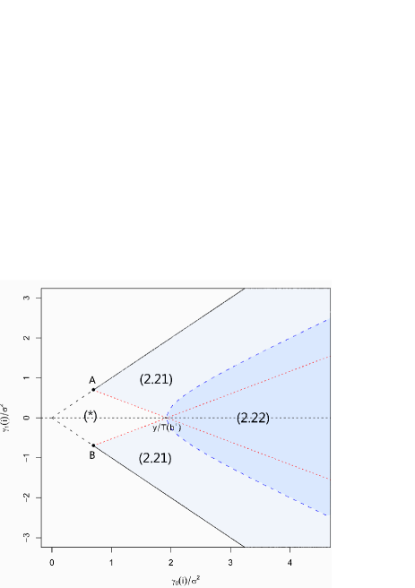
Figure 2: Region of $\gamma_{0}(i)/\sigma^{2}$ and $\gamma_{1}(i)/\sigma^{2}$ that will lead to significant factors.

We summarize the above findings as follows.

Corollary 2.2.

Under the same conditions as in Theorem 2.1, the $i$-th time series $(x_{it})$ will generate a significant factor in the sense that $T_{1}(i)<T(b^{+})$ if and only if either

$$\frac{|\gamma_{1}(i)|}{\sigma^{2}}>\tau_{0},$$ (2.25)

or

$$\frac{|\gamma_{1}(i)|}{\sigma^{2}}\leq\tau_{0}\quad\text{and}\quad\frac{\gamma_{0}(i)}{\sigma^{2}}>\frac{y-\sqrt{T^{2}(b^{+})+T(b^{+})}|\gamma_{1}(i)|/\sigma^{2}}{T(b^{+})},$$ (2.26)

where the constant $\tau_{0}$ is given in (2.24).

We now introduce some important comments on the meaning of these conditions.

1. The essential message from these conditions is that the $i$-th factor time series is a significant factor once its strength $\gamma_{0}(i)$, or more exactly, its SNR $\gamma_{0}(i)/\sigma^{2}$ exceeds a certain level $\tau$. A sufficient value for this level $\tau$ is $\tau_{1}=y/T(b^{+})$ as shown in Figure 2. Meanwhile, the SNR should at least equal to $\tau_{0}$ given in (2.24), see Point A on the figure which has coordinates $(\tau_{0},\tau_{0})$. When $\tau_{0}<\gamma_{0}(i)/\sigma^{2}\leq\tau_{1}$, the exact condition also depends on the lag-1 SNR $|\gamma_{1}(i)|/\sigma^{2}$ as given in Eqs. (2.25)-(2.26).

   This is thus much in line with what is known for the phase transition phenomenon for large sample covariance matrices as exposed in [7] and [6].

2. As said in Introduction, in most of existing literature on high-dimensional factor models, the factor strengths are assumed to grow to infinity with the dimension $p$. Clearly, such growing factors are highly significant in our scheme, i.e. $k_{0}=k$, since they will exceed the upper limit $\tau_{1}$ very quickly as the dimension $p$ grows.

3. Assume that $y\to 0_{+}$, i.e. the sample size $T$ is much larger than the dimension $p$. Then it can be checked that both the quantities $\tau_{0}$ and $\tau_{1}$ will vanish. Therefore, when $p/T$ is small enough, any factor time series will generate a significant sample factor eigenvalue. In other words, we have recovered the classical low-dimensional situation where $p$ is hold fixed and $T\to\infty$ for which all the $k$ factor time series can be consistently detected and identified.

3 Estimation of the number of factors

Let $l_{1},\cdots,l_{p}$ be the eigenvalues of $\widehat{M}=\widehat{\Sigma}_{y}{}\widehat{\Sigma}_{y}{}^{\prime}$, sorted in decreasing order. Assume that among the $k$ factors, the first $k_{0}$ are significant which satisfy the phase transition condition $T_{1}(i)<T(b^{+})$, see Eq.(2.8). Following Theorem 2.1, the $k$ largest sample eigenvalue $(l_{i}/\sigma^{4})_{1\leq i\leq k}$ converges respectively to a limit $(\lambda_{i})$, which is larger than the right edge $b$ of the limiting spectral distribution for $1\leq i\leq k_{0}$, and equal to $b$ for $k_{0}<i\leq k$.

It will be proved below that the largest noise sample eigenvalues of a given finite number all converge to $b$, i.e. for any fixed range $m>0$,

$$l_{k+1}/\sigma^{4}\to b,\leavevmode\nobreak\ \ldots\leavevmode\nobreak\ ,l_{k+m}/\sigma^{4}\to b,\quad\text{almost surely}.$$ (3.1)

Consider the sequence of ratios

$${\color[rgb]{0,0,0}\theta_{j}:=\frac{l_{j+1}/\sigma^{4}}{l_{j}/\sigma^{4}}=\frac{l_{j+1}}{l_{j}},\quad j\geq 1.}$$ (3.2)

By definition $\theta_{j}\leq 1$. Therefore, we have almost surely,

$$\theta_{j}\rightarrow\frac{\lambda_{j+1}}{\lambda_{j}}<1\leavevmode\nobreak\ ,\leavevmode\nobreak\ \leavevmode\nobreak\ \leavevmode\nobreak\ \leavevmode\nobreak\ j<k_{0}\leavevmode\nobreak\ ,$$

$$\theta_{k_{0}}\rightarrow\frac{b}{\lambda_{k_{0}}/\sigma^{4}}<1\leavevmode\nobreak\ ,$$ (3.3)

$$\theta_{j}\rightarrow\frac{b}{b}=1\leavevmode\nobreak\ ,\leavevmode\nobreak\ \leavevmode\nobreak\ \leavevmode\nobreak\ \leavevmode\nobreak\ k_{0}<j\leq k\leavevmode\nobreak\ ,$$

$$\theta_{k+1},\leavevmode\nobreak\ \ldots,\leavevmode\nobreak\ \theta_{k+m}\rightarrow\frac{b}{b}=1\leavevmode\nobreak\ ,\quad\text{for all fixed \leavevmode\nobreak\ }m.$$

Remark 3.1.

Note that the value of $\theta_{j}$ is independent of $\sigma^{2}$. In other words, we do not need the true value of $\sigma^{2}$ for estimating the number of factors, indeed.

Let $0<d_{T}<1$ be a positive constant and we introduce the following estimator for the number of factors $k$:

$$\widehat{k}=\{\text{first}\leavevmode\nobreak\ j\geq 1\leavevmode\nobreak\ \leavevmode\nobreak\ \text{such that }\leavevmode\nobreak\ \theta_{j}>1-d_{T}\}-1\leavevmode\nobreak\ .$$ (3.4)

Theorem 3.1.

Consider the factor model (1.1) and assume that the same conditions as in Theorem 2.1 are satisfied. Let $k_{0}$ be the number of significant factors defined in Eq. (2.8) and a threshold constant $d_{T}$ be chosen such that

$$\max_{1\leq j\leq k_{0}}\lambda_{j+1}/\lambda_{j}<1-d_{T}<1.$$ (3.5)

Then $\widehat{k}\xrightarrow{a.s}k_{0}$.

This theorem thus formally establishes the fact that the ratio estimator $\widehat{k}$ is able to detect all the significant factors that satisfy the phase transition condition given in Theorem 2.1 and detailed in Eqs.(2.25)-(2.26).

Proof.

(of Theorem 3.1)  As $\theta_{j}\xrightarrow{a.s.}\lambda_{j+1}/\lambda_{j}$ for $1\leq j\leq k_{0}$ and by assumption (3.5), almost surely, it will happen eventually that $\widehat{k}>k_{0}$. Next, under the claim (3.1) and following the limits given in (3.3),

$$\theta_{j}\xrightarrow{a.s.}1,\quad\text{for }j>k_{0}.$$ (3.6)

Consequently, almost surely we will have eventually $\widehat{k}\leq k_{0}$ which, combined with the conclusion above, proves the almost sure convergence of $\widehat{k}$ to $k_{0}$.

It remains to prove the claim (3.1). Since $\theta_{j}$ is independent of the choice of $\sigma^{2}$, we can assume w.l.o.g that $\sigma^{2}=1$ as before. Recall that in the proof of Theorem 2.1, it has been proved in Eqs.(2.13)-(2.14) that if $l$ is a eigenvalue of $\widehat{M}$, then $\sqrt{l}$ is a positive eigenvalue of the matrix

$$\Gamma=\left(\begin{array}[]{cccc}0&X_{1}^{\prime}X_{0}&0&X_{1}^{\prime}E_{1}\\ X_{0}^{\prime}X_{1}&0&X_{0}^{\prime}E_{2}&0\\ 0&E_{2}^{\prime}X_{0}&0&E_{2}^{\prime}E_{1}\\ E_{1}^{\prime}X_{1}&0&E_{1}^{\prime}E_{2}&0\end{array}\right)\leavevmode\nobreak\ ,$$

which is obtained after permutation of the second and third row block and column block in (2.14) without modifying the eigenvalues. Now $\Gamma$ is a symmetric block matrix and the positive eigenvalues of the lower diagonal block

$$\left(\begin{array}[]{cc}0&E_{2}^{\prime}E_{1}\\ E_{1}^{\prime}E_{2}&0\end{array}\right)\leavevmode\nobreak\ ,$$

are associated to the eigenvalues of the matrix $DD^{\prime}=E_{2}^{\prime}E_{1}E_{1}^{\prime}E_{2}$ which is of dimension $p-k$ (for the definition of these matrices, see that proof). Let $\beta_{1}\geq\cdots\geq\beta_{p-k}$ be the eigenvalues of $DD^{\prime}$. By Cauchy interlacing theorem, we have

$$\beta_{k+1}\leq l_{k+1}\leq\beta_{1}.$$

Observing that $D$ is distributed as $\widehat{\Sigma}_{\varepsilon}{}$ except that the dimension is changed from $p$ to $p-k$. Therefore, the global limit of the eigenvalues of $DD^{\prime}$ are the same as for the matrix $\widehat{\Sigma}_{\varepsilon}{}\widehat{\Sigma}_{\varepsilon}{}^{\prime}$; in particular, according to Corollary 2.1, both $\beta_{k+1}$ and $\beta_{1}$ converge to $b$ almost surely. This proves the fact that $l_{k+1}\xrightarrow{a.s}b$. Using similar arguments, we can establish the same fact for $l_{k+j}\xrightarrow{a.s}b$ for any fixed index $j\geq 1$. The claim (3.1) is thus established. ∎

3.1 Calibration of the tuning parameter $d_{T}$

For the estimator $\widehat{k}$ in (3.4) to be practically useful, we need to set up an appropriate value of the tuning parameter $d_{T}$. Although in theory, any vanishing sequence $d_{T}\to 0$ will guarantee the consistence of $\widehat{k}$, it is preferable to have an indicated and practically useful sequence $(d_{T})$ for real-life data analysis. Here we propose an a priori calibration of $d_{T}$ based on some knowledge from random matrix theory on the largest eigenvalues of sample covariance matrices and of their perturbed versions. The most important property we will use is that according to such recent results on finite rank perturbations of symmetric random matrices, see e.g. Benaych-Georges et al. [9] it is very likely that the asymptotic distribution of $T^{\frac{2}{3}}\left(\dfrac{l_{k+2}}{l_{k+1}}-1\right)$ is the same as that of $T^{\frac{2}{3}}\left(\dfrac{\nu_{2}}{\nu_{1}}-1\right)$, where $\nu_{1}$, $\nu_{2}$ are the two largest eigenvalues of the base noise matrix $\widehat{M}_{\varepsilon}$. Using this similarity, we calibrate $d_{T}$ by simulation: for any given pair $(p,T)$, the distribution of $T^{\frac{2}{3}}\left(\dfrac{\nu_{2}}{\nu_{1}}-1\right)$ is sampled using a large number (in fact 2000) of independent replications of standard Gaussian vectors $\varepsilon_{t}\sim N({\bf 0},{\bf I}_{p})$ and its lower 0.5% quantile $q_{p,T,0.5\%}$ is obtained (notice that the quantile is negative). Using the approximation

$$P\left\{T^{\frac{2}{3}}\left(\dfrac{l_{k+2}}{l_{k+1}}-1\right)\leq q_{p,T,0.5\%}\right\}\simeq P\left\{T^{\frac{2}{3}}\left(\dfrac{\nu_{2}}{\nu_{1}}-1\right)\leq q_{p,T,0.5\%}\right\}=0.5\%,$$

we calibrate $d_{T}$ at the value $d_{T}=|q_{p,T,0.5\%}|/T^{2/3}$. Notice that $d_{T}$ vanishes at rate $T^{-2/3}$. In all the simulation experiments in Section 4 or for the data analysis reported in Section 5, this tuned value of $d_{T}$ is used for the given pairs $(T,p)$.

4 Monte-Carlo experiments

In this section, we report some simulation results to show the finite-sample performance of our estimator. For the reason of robustness, we will consider a reinforced estimator $\widehat{k}^{*}$ defined as

$$\widehat{k}^{*}=\{\text{first}\leavevmode\nobreak\ j\geq 1\leavevmode\nobreak\ \leavevmode\nobreak\ \text{such that }\leavevmode\nobreak\ \theta_{j}>1-d_{T}\leavevmode\nobreak\ \text{and }\leavevmode\nobreak\ \theta_{j+1}>1-d_{T}\}-1\leavevmode\nobreak\ .$$ (4.1)

Clearly, $\widehat{k}^{*}$ is asymptotically equivalent to the initial estimator $\widehat{k}$ which uses only one single test value $j$. As for the factor model, we adopt the same settings as in [17] where

$$y_{t}=Ax_{t}+\varepsilon_{t},\leavevmode\nobreak\ \varepsilon_{t}\sim N_{p}({\bf 0},{\bf I}_{p}),$$

$$x_{t}=\Theta x_{t-1}+e_{t},\leavevmode\nobreak\ e_{t}\sim N_{k}({\bf 0},\Gamma),$$

where $A$ is a $p\times k$ matrix, w.l.o.g, we set the variance $\sigma^{2}$ of the white noise $\varepsilon_{t}$ to be 1.

In [17], the factor loading matrix $A$ are independently generated from uniform distribution on the interval $[-1,1]$ first and then divided by $p^{\delta/2}$ where $\delta\in[0,1]$. The induced $k$ factor strengths are thus of order $O(p^{1-\delta})$. Their estimator of number of factors is recalled in (1.4). Cases where three factors are either all very strong with $\delta=0$ or all moderately strong with $\delta=0.5$ are discussed in details in that paper. The results show that $\tilde{k}$ performs better when factors are stronger. An experimental setting with a combination of two strong factors and one moderate factor indicates that a two-step estimation procedure needs to be employed in order to identify all three factors. In each step only factors with the highest level of strength can be detected.

While in our case, the coefficient matrix $A$ satisfies $A^{\prime}A=I_{k}$. Considering the eigenvalues of $\widehat{M}$ are invariant under orthogonal transformation (See Step 2 in the proof of Theorem 2.1), we fix

$$A=\begin{pmatrix}I_{k}\\ \bm{0}_{p-k}\\ \end{pmatrix}\leavevmode\nobreak\ .$$

Then we manipulate the factor strength by adjusting the value of $\Theta$ and $\Gamma$. To ensure the stationarity of $\{y_{t}\}$ process and the Independence among the components of the factor process $\{x_{t}\}$, $\Theta$ and $\Gamma$ are both diagonal matrices and the diagonal elements of $\Theta$ lie within $(-1,1)$. To keep pace with the settings in [17], we multiply $p^{\frac{1-\delta}{2}}$ with the diagonal entries of $\Gamma$ to adjust the corresponding factor strength. It can be seen that when $\delta=0$, the factor is strongest while with $\delta=1$, the factor is weakest.

The entire simulation study is mainly composed of four parts formulated in four different scenarios as follows:

• Two very strong factors with $\delta_{1}=0.5$ and $\delta_{2}=0.8$ and

  $$\leavevmode\nobreak\ \Theta=\left(\begin{array}[]{cc}0.6&0\\ 0&0.5\end{array}\right),\leavevmode\nobreak\ \Gamma=\left(\begin{array}[]{cc}4\times p^{\frac{1-\delta_{1}}{2}}&0\\ 0&4\times p^{\frac{1-\delta_{2}}{2}}\end{array}\right).$$

• Four weak factors with same strength level $\delta=1$; three of them are significant with their theoretical limits $\lambda_{1},\leavevmode\nobreak\ \lambda_{2},\leavevmode\nobreak\ \lambda_{3}$ all keeping a moderate distance from $b$ while the fourth factor is insignificant with its theoretical limit $\lambda_{4}$ equal to right edge $b$ of the noise eigenvalues. Precisely,

  $$\leavevmode\nobreak\ \Theta=\left(\begin{array}[]{cccc}0.6&0&0&0\\ 0&-0.5&0&0\\ 0&0&0.3&0\\ 0&0&0&0.2\end{array}\right),\leavevmode\nobreak\ \Gamma=\left(\begin{array}[]{cccc}4&0&0&0\\ 0&4&0&0\\ 0&0&4&0\\ 0&0&0&1\end{array}\right).$$

• Three weak factors with $\delta=1$ and $\lambda_{3}$ stays very close to $b$ and

  $$\leavevmode\nobreak\ \Theta=\left(\begin{array}[]{ccc}0.6&0&0\\ 0&-0.5&0\\ 0&0&0.3\end{array}\right),\leavevmode\nobreak\ \Gamma=\left(\begin{array}[]{ccc}2&0&0\\ 0&2&0\\ 0&0&2\end{array}\right).$$

• A mixed case with two strong factors with $\delta_{1}=0.5,\leavevmode\nobreak\ \delta_{2}=0.8$, and five weak factors with $\delta=1$, and

  $$\Theta=diag(0.6,0.5,0.6,-0.5,0.3,0.6,-0.5),$$

  $$\Gamma=diag(4\times p^{\frac{1-\delta_{1}}{2}},4\times p^{\frac{1-\delta_{2}}{2}},4,4,4,2,2).$$

Recall that for the estimator $\widehat{k}^{*}$, the critical value $d_{T}$ is calibrated as explained in Section 3.1 using the simulated empirical 0.5% lower quantile. We set $p=100,\leavevmode\nobreak\ 300,\leavevmode\nobreak\ 500,\leavevmode\nobreak\ 1000,\leavevmode\nobreak\ 1500$, $T=0.5p,\leavevmode\nobreak\ 2p$, i.e $y=2,\leavevmode\nobreak\ 0.5$. It will be seen below that in general, the cases with $T=0.5p$ will be harder to deal with than the cases with $T=2p$. We repeat 1000 times to calculate the empirical frequencies of the different decisions $(\widehat{k}^{*}=k_{0})$, $(\widehat{k}^{*}=k_{0}\pm 1)$ and $(|\widehat{k}^{*}-k_{0}|>1)$. The results are as follows.

• In Scenario I, we have two very strong factors with $\delta_{1}=0.5$ and $\delta_{2}=0.8$ and their strengths grow to infinity with $p$. Thus $k_{0}=k=2$ and the two factors must be easily detectable. As seen from Table 1, our estimator $\widehat{k}^{*}$ converges very fast to the true number of factors. On the other hand, the one-step estimator $\tilde{k}$ of Lam and Yao [17] tends to detect only one factor in each step due to the fact that the two factors are of different strength.

  Table 1: Scenario I with two strong factors ($k_{0}=k=2$)

  $p$	100	300	500	1000	1500	$p$	100	300	500	1000	1500
  $T=2p$	200	600	1000	2000	3000	$T=2p$	200	600	1000	2000	3000
  $\tilde{k}=1$	0.343	0.294	0.257	0.287	0.317	$\widehat{k}^{*}=1$	0	0	0	0	0
  $\tilde{k}=k_{0}$	0.657	0.706	0.743	0.713	0.683	$\widehat{k}^{*}=k_{0}$	0.974	0.984	0.993	0.996	0.998
  $\tilde{k}\geq 3$	0	0	0	0	0	$\widehat{k}^{*}\geq 3$	0.026	0.016	0.007	0.004	0.002
  $p$	100	300	500	1000	1500	$p$	100	300	500	1000	1500
  $T=0.5p$	50	150	250	500	750	$T=0.5p$	50	150	250	500	750
  $\tilde{k}=1$	0.786	0.801	0.876	0.96	0.992	$\widehat{k}^{*}=1$	0.086	0	0	0	0
  $\tilde{k}=k_{0}$	0.21	0.199	0.124	0.04	0.008	$\widehat{k}^{*}=k_{0}$	0.771	0.882	0.896	0.881	0.881
  $\tilde{k}\geq 3$	0.004	0	0	0	0	$\widehat{k}^{*}\geq 3$	0.143	0.118	0.104	0.119	0.119

• In Scenario II, we have four weak factors of same strength level $\delta=1$. The theoretical limits related to Theorem 2.1 are displayed in Table 2. Figure 3 for $T=2p$ and Figure 4 for $T=0.5p$ depict the position of these four factors (numbered from 1 to 4) in the phase transition region defined in Corollary 2.2 and we see three among the four lying inside the detectable area in both situations. It can be seen from the table that for both combinations of $T=2p$ and $T=0.5p$, the first three limits $\lambda_{i}$ are far from upper bound $b$ and the fourth limit $\lambda_{4}$ equals to $b$. We thus have three significant factors ($k_{0}=3$) which are detectable while the fourth one is too weak for the detection. Results in Table 3 show that both the estimators $\tilde{k}$ (one-step) and $\widehat{k}^{*}$ are consistent with however a much higher convergence speed for $\widehat{k}^{*}$.

  Table 2: Scenario II - Theoretical limits ($k_{0}=3,\leavevmode\nobreak\ k=4$)

  					$T=2p$				$T=0.5p$
  No.	$\Theta$	$\Gamma$	$\gamma_{0}\left(i\right)$	$\gamma_{1}\left(i\right)$	$T_{1}(i)$	$T(b^{+})$	$\lambda_{i}$	$b$	$T_{1}(i)$	$T(b^{+})$	$\lambda_{i}$	$b$
  (1)	0.6	4	6.25	3.75	0.0125	0.3076	21.2	2.7725	0.1102	0.7775	44.8	17.6366
  (2)	-0.5	4	5.33	-2.67	0.021	0.3076	13.1	2.7725	0.1596	0.7775	33.85	17.6366
  (3)	0.3	4	4.3956	1.3187	0.047	0.3076	6.65	2.7725	0.2767	0.7775	23.92	17.6366
  (4)	0.2	1	1.042	0.2083	0.3446	0.3076	2.7725	2.7725	1.5296	0.7775	17.6366	17.6366

  

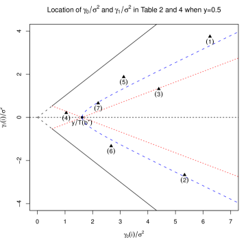
  Figure 3: Locations of factor SNR’s $(\gamma_{0}/,\gamma_{1})/\sigma^{2}$ from Tables 2 (points numbered from 1 to 4), 4 (points numbered from 5 to 7), and 6 (points numbered 1-2-3-5-6) with $T=2p$ ($y=0.5$).

  

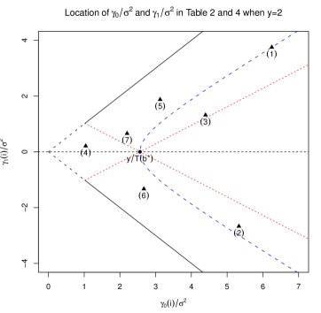
  Figure 4: Locations of factor SNR’s $(\gamma_{0}/,\gamma_{1})/\sigma^{2}$ from Tables 2 (points numbered from 1 to 4), 4 (points numbered from 5 to 7), and 6 (points numbered 1-2-3-5-6) with $T=0.5p$ ($y=2$).

  Table 3: Scenario II with three weak yet significant factors among four $(k_{0}=3,\leavevmode\nobreak\ k=4$)

  p	100	300	500	1000	1500	p	100	300	500	1000	1500
  T=2p	200	600	1000	2000	3000	T=2p	200	600	1000	2000	3000
  $\tilde{k}=1$	0.152	0.074	0.045	0.01	0.001	$\widehat{k}^{*}=1$	0.005	0	0	0	0
  $\tilde{k}=2$	0.402	0.344	0.276	0.194	0.126	$\widehat{k}^{*}=2$	0.026	0	0	0	0
  $\tilde{k}=k_{0}$	0.446	0.582	0.679	0.796	0.873	$\widehat{k}^{*}=k_{0}$	0.928	0.967	0.953	0.96	0.966
  $\tilde{k}=4$	0	0	0	0	0	$\widehat{k}^{*}=4$	0.04	0.033	0.046	0.04	0.033
  $\tilde{k}\geq 5$	0	0	0	0	0	$\widehat{k}^{*}\geq 5$	0.001	0	0.001	0	0.001
  p	100	300	500	1000	1500	p	100	300	500	1000	1500
  T=0.5p	50	150	250	500	750	T=0.5p	50	150	250	500	750
  $\tilde{k}=1$	0.479	0.368	0.344	0.284	0.289	$\widehat{k}^{*}=1$	0.376	0.02	0.003	0	0
  $\tilde{k}=2$	0.406	0.432	0.454	0.495	0.514	$\widehat{k}^{*}=2$	0.456	0.221	0.048	0.001	0
  $\tilde{k}=k_{0}$	0.105	0.199	0.202	0.221	0.197	$\widehat{k}^{*}=k_{0}$	0.16	0.73	0.915	0.986	0.982
  $\tilde{k}=4$	0.006	0.001	0	0	0	$\widehat{k}^{*}=4$	0.008	0.029	0.03	0.013	0.017
  $\tilde{k}\geq 5$	0.004	0	0	0	0	$\widehat{k}^{*}\geq 5$	0	0	0.004	0	0.001

• Theoretical limits and empirical result for Scenario III are presented in Table 4, Figures 3 and 4, and Table 5. For both situations of $T=0.5p$ and $T=2p$, the model has three significant factors ($k_{0}=k=3$). Notice however that when $T=0.5p$, the 3rd factor is quite weak and the corresponding limit $\lambda_{3}=17.95$ is very close to the right edge $b=17.64$ so that this factor would be detectable only in theory (or with very large sample sizes). This is also easily verified in Figure 4 that the point (3) corresponding to the weakest factor lies very close to the boundary of the detectable region. As for the empirical values in Table 5, the estimator $\widehat{k}^{*}$ converges quickly when $T=2p$ and much more slowly when $T=0.5p$. Meanwhile, the estimator $\tilde{k}$ (with one-step) seems inconsistent even in the easier case of $T=2p$.

  Table 4: Scenario III - Theoretical limits ($k_{0}=k=3$)

  					$T=2p$				$T=0.5p$
  No.	$\Theta$	$\Gamma$	$\gamma_{0}\left(i\right)$	$\gamma_{1}\left(i\right)$	$T_{1}(i)$	$T(b^{+})$	$\lambda_{i}$	$b$	$T_{1}(i)$	$T(b^{+})$	$\lambda_{i}$	$b$
  (5)	0.6	2	3.125	1.875	0.0391	0.3076	7.65	2.7725	0.2845	0.7775	23.79	17.6366
  (6)	-0.5	2	2.67	-1.33	0.0607	0.3076	5.48	2.7725	0.3852	0.7775	20.45	17.6366
  (7)	0.3	2	2.20	0.659	0.1183	0.3076	3.61	2.7725	0.6116	0.7775	17.95	17.6366

  Table 5: Scenario III with three weak yet insignificant factors ($k_{0}=k=3$)

  $p$	100	300	500	1000	1500	$p$	100	300	500	1000	1500
  $T=2p$	200	600	1000	2000	3000	$T=2p$	200	600	1000	2000	3000
  $\tilde{k}<2$	0.403	0.322	0.327	0.302	0.308	$\widehat{k}^{*}<2$	0.074	0	0	0	0
  $\tilde{k}=2$	0.454	0.587	0.598	0.653	0.669	$\widehat{k}^{*}=2$	0.441	0.047	0.005	0	0
  $\tilde{k}=k_{0}$	0.143	0.091	0.075	0.045	0.023	$\widehat{k}^{*}=k_{0}$	0.48	0.945	0.991	0.996	0.999
  $\tilde{k}\geq 4$	0	0	0	0	0	$\widehat{k}^{*}\geq 4$	0.005	0.008	0.004	0.004	0.001
  $p$	100	300	500	1000	1500	$p$	100	300	500	1000	1500
  $T=0.5p$	50	150	250	500	750	$T=0.5p$	50	150	250	500	750
  $\tilde{k}<2$	0.548	0.57	0.589	0.548	0.547	$\widehat{k}^{*}<2$	0.886	0.639	0.435	0.114	0.049
  $\tilde{k}=2$	0.264	0.359	0.371	0.437	0.447	$\widehat{k}^{*}=2$	0.107	0.338	0.508	0.718	0.745
  $\tilde{k}=k_{0}$	0.08	0.053	0.036	0.015	0.006	$\widehat{k}^{*}=k_{0}$	0.006	0.022	0.057	0.167	0.205
  $\tilde{k}\geq 4$	0.108	0.018	0.004	0	0	$\widehat{k}^{*}\geq 4$	0.001	0.001	0	0.001	0.001

• Scenario IV is the most complex case with two very strong factors and five weak factors. As predicted by the theory, the two largest factor eigenvalues $l_{1},\leavevmode\nobreak\ l_{2}$ of $\widehat{M}$ blow up to infinity while the following 5 factor eigenvalues $l_{3}\sim l_{7}$ converge to a $\lambda_{i}>b$. The corresponding theoretical limits for the five weak factors are given in Table 6 and their SNR’s depicted in Figures 3 and 4. Meanwhile, all the $k_{0}=k=7$ factors are significant. Clearly in this scenario, the performance of the one-step estimator $\tilde{k}$, denoted as $\tilde{k}^{(1)}$, is quite limited and in order to make a closer comparison with our estimator $\widehat{k}^{*}$, we have also run the two-step and the three-step versions of the estimator $\tilde{k}$. Among these two versions we report the best results obtained by the three-step version (denoted as $\tilde{k}^{(3)}$). It can be seen from Table 7 that our estimator is able to detect the 7 factors with multi-level strength in a single step while $\tilde{k}$ can only identify one factor in each step: i.e. $\tilde{k}^{(1)}\rightarrow 1$ and $\tilde{k}^{(3)}\rightarrow 3$.

  Table 6: Scenario IV - Theoretical limits ($k_{0}=k=7$)

  					$T=2p$				$T=0.5p$
  NO.	$\Theta$	$\Gamma$	$\gamma_{0}\left(i\right)$	$\gamma_{1}\left(i\right)$	$T_{1}(i)$	$T\left(b^{+}\right)$	$\lambda_{i}$	$b$	$T_{1}(i)$	$T\left(b^{+}\right)$	$\lambda_{i}$	$b$
  (1)	0.6	4	6.25	3.75	0.0125	0.3076	21.2	2.7725	0.1102	0.7775	44.8	17.6366
  (2)	-0.5	4	5.33	-2.67	0.021	0.3076	13.1	2.7725	0.1596	0.7775	33.85	17.6366
  (3)	0.3	4	4.3956	1.3187	0.047	0.3076	6.65	2.7725	0.2767	0.7775	23.92	17.6366
  (5)	0.6	2	3.125	1.875	0.0391	0.3076	7.65	2.7725	0.2845	0.7775	23.79	17.6366
  (6)	-0.5	2	2.67	-1.33	0.0607	0.3076	5.48	2.7725	0.3852	0.7775	20.45	17.6366

  Table 7: Scenario IV with seven factors of multiple strength levels ($k_{0}=k=7$)

  p	100	300	500	1000	1500	p	100	300	500	1000	1500
  T=2p	200	600	1000	2000	3000	T=0.5p	50	150	250	500	750
  $\tilde{k}^{(1)}=1$	0.696	0.858	0.949	0.995	1	$\tilde{k}^{(1)}=1$	0.73	0.812	0.881	0.95	0.986
  $\tilde{k}^{(1)}=2$	0.244	0.137	0.051	0.005	0	$\tilde{k}^{(1)}=2$	0.211	0.177	0.118	0.05	0.014
  $\tilde{k}^{(1)}=3$	0.033	0.004	0	0	0	$\tilde{k}^{(1)}=3$	0.039	0.011	0.001	0	0
  $\tilde{k}^{(1)}=4$	0.019	0.001	0	0	0	$\tilde{k}^{(1)}=4$	0.015	0	0	0	0
  $\tilde{k}^{(1)}=5$	0.005	0	0	0	0	$\tilde{k}^{(1)}=5$	0.004	0	0	0	0
  $\tilde{k}^{(1)}=6$	0.002	0	0	0	0	$\tilde{k}^{(1)}=6$	0.001	0	0	0	0
  $\tilde{k}^{(1)}=k_{0}$	0.001	0	0	0	0	$\tilde{k}^{(1)}=k_{0}$	0	0	0	0	0
  $\tilde{k}^{(1)}\geq 8$	0	0	0	0	0	$\tilde{k}^{(1)}\geq 8$	0	0	0	0	0
  p	100	300	500	1000	1500	p	100	300	500	1000	1500
  T=2p	200	600	1000	2000	3000	T=0.5p	50	150	250	500	750
  $\tilde{k}^{(3)}=1$	0	0	0	0	0	$\tilde{k}^{(3)}=1$	0	0	0	0	0
  $\tilde{k}^{(3)}=2$	0	0	0	0	0	$\tilde{k}^{(3)}=2$	0	0	0	0	0
  $\tilde{k}^{(3)}=3$	0.691	0.875	0.945	0.998	0.999	$\tilde{k}^{(3)}=3$	0.71	0.802	0.862	0.955	0.982
  $\tilde{k}^{(3)}=4$	0.002	0	0	0	0	$\tilde{k}^{(3)}=4$	0	0	0	0	0
  $\tilde{k}^{(3)}=5$	0	0	0	0	0	$\tilde{k}^{(3)}=5$	0.001	0	0	0	0
  $\tilde{k}^{(3)}=6$	0.244	0.125	0.055	0.002	0.001	$\tilde{k}^{(3)}=6$	0.212	0.192	0.135	0.045	0.018
  $\tilde{k}^{(3)}=k_{0}$	0	0	0	0	0	$\tilde{k}^{(3)}=k_{0}$	0	0	0	0	0
  $\tilde{k}^{(3)}\geq 8$	0.063	0	0	0	0	$\tilde{k}^{(3)}\geq 8$	0.077	0.006	0.003	0	0
  p	100	300	500	1000	1500	p	100	300	500	1000	1500
  T=2p	200	600	1000	2000	3000	T=0.5p	50	150	250	500	750
  $\widehat{k}^{*}=1$	0.012	0	0	0	0	$\widehat{k}^{*}=1$	0.151	0.01	0	0	0
  $\widehat{k}^{*}=2$	0.031	0.001	0	0	0	$\widehat{k}^{*}=2$	0.25	0.038	0.01	0.001	0
  $\widehat{k}^{*}=3$	0.034	0.002	0	0	0	$\widehat{k}^{*}=3$	0.28	0.065	0.027	0.003	0
  $\widehat{k}^{*}=4$	0.062	0.015	0.006	0.001	0	$\widehat{k}^{*}=4$	0.254	0.227	0.107	0.022	0.007
  $\widehat{k}^{*}=5$	0.049	0	0	0	0	$\widehat{k}^{*}=5$	0.06	0.384	0.295	0.035	0.002
  $\widehat{k}^{*}=6$	0.185	0	0	0	0	$\widehat{k}^{*}=6$	0.005	0.231	0.414	0.34	0.138
  $\widehat{k}^{*}=k_{0}$	0.597	0.939	0.958	0.95	0.959	$\widehat{k}^{*}=k_{0}$	0	0.044	0.142	0.557	0.783
  $\widehat{k}^{*}\geq 8$	0.03	0.043	0.036	0.049	0.041	$\widehat{k}^{*}\geq 8$	0	0.001	0.005	0.042	0.07

5 An example of real data analysis

We analyse the log returns of 100 stocks (denoted by $y_{t}$), included in the S&P500 during the period from 2005-01-03 to 2011-09-16. We have in total $T=1689$ observations with $p=100$. Thorough eigenvalue analysis is applied to the lag-1 sample auto-covariance matrix $\widehat{M}=\widehat{\Sigma}_{y}{}\widehat{\Sigma}^{\prime}_{y}{}$ of $y_{t}$. The largest eigenvalue of $\widehat{M}$ is $\lambda_{1}(\widehat{M})=38.69$. The second to the 30th largest eigenvalues and their ratios are plotted in Fig 5.

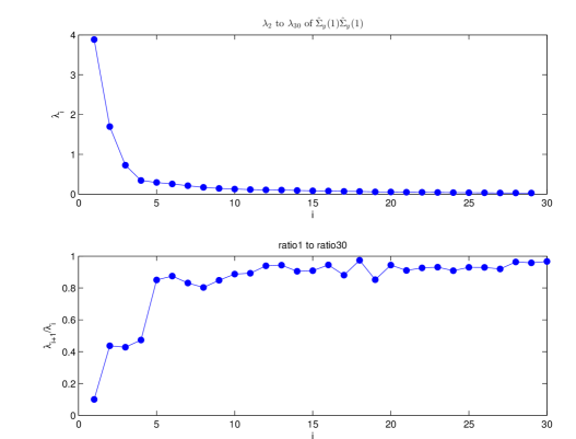
Figure 5: Eigenvalues of $\widehat{M}$

To estimate the number of factors, we first adopt the two-step procedure investigated by Lam and Yao [17] since the ratio plot in Fig 5 is exhibiting at least two different levels of factor strength. Obviously, in the first step,

$$\widehat{r}_{1}=\underset{1\leq i\leq 99}{\arg\min}\lambda_{i+1}/\lambda_{i}=1,$$

the factor loading estimator of the first factor $\widehat{A}$ is the eigenvector of $\widehat{M}$ which corresponds to the largest eigenvalue $\lambda_{1}$. The resulting residuals after eliminating the effect of the first factor is

$$\widehat{\varepsilon}_{t}=({\bf I}_{100}-\widehat{A}\widehat{A}^{\prime})y_{t}.$$

Repeating the procedure in step one, we treat $\widehat{\varepsilon}$ as the original sequence $y_{t}$ and get the eigenvalues $\lambda_{i}^{*}s$ of the lag-1 sample auto-covariance matrix $\widehat{M}^{(1)}=\widehat{\Sigma}_{\widehat{\varepsilon}}{}\widehat{\Sigma}^{\prime}_{\widehat{\varepsilon}}{}$. The 30 largest eigenvalues and their ratios are plotted in Fig 6.

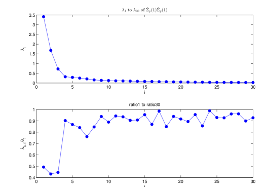
Figure 6: Eigenvalues of $\widehat{M}^{(1)}$

It can be seen from the second step that

$$\widehat{r}_{2}=\underset{1\leq i\leq 99}{\arg\min}\lambda^{*}_{i+1}/\lambda^{*}_{i}=2,$$

the factor loading estimator of the second level factors $\widehat{A}^{*}$ are the orthonormal eigenvectors of $\widehat{M}^{(1)}$ corresponding to the first two largest eigenvalues.

In conclusion, the two-step procedure proposed by [17] identifies three factors in total with two different levels of factor strength. The eigenvalues of the lag-1 sample auto-covariance matrix $\widehat{M}^{(2)}$ of residuals after subtracting the three factors detected previously are shown in Fig 7.

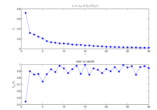
Figure 7: Eigenvalues of $\widehat{M}^{(2)}$

There is still one isolated eigenvalue in the eigenvalues plot. If we go one step further and treat it as an extra factor with weakest strength, then the eigenvalue plot of the lag-1 sample auto-covariance matrix $\widehat{M}^{(3)}$ of residuals after eliminating four factors looks like in Fig 8.

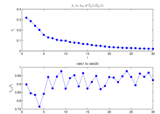
Figure 8: Eigenvalues of $\widehat{M}^{(3)}$

A major problem of the methodology in [17] is that it does not provide a clear criterion to stop this two or multi-step procedure. Clearly, this method can only detect factors with one level of strength at each step and can hardly handle problems with factors of multilevel strengths due to the lack of stopping criterion in multi-step detection.

In the following, we use the estimator $\widehat{k}^{*}$ (4.1) of this paper to estimate the number of factors. At first, the tuning parameter $d_{T}$ is calibrated with $(p,T)=(100,1689)$ using the simulation method indicated in Section 3.1; the value found is $d_{T}=0.1713$ in this case. The eigenvalue ratios of the sample matrix $\widehat{M}$ are shown in Figure 9 (already displayed in the lower panel of Figure 5) where the detection line of value $1-d_{T}=0.8287$ is also drawn. As displayed, we found $\widehat{k}^{*}=4$ factors.

In conclusion, for this data set with $p=100$ stocks, our estimator proposes 4 significant factors while the estimator $\tilde{k}$ from [17] indicate 1, 3 and 4 factors when one step, two steps and 3 steps are used respectively. It appears again that multiple steps are needed for the use of the estimator $\widehat{k}$ in real data analysis; it remains however unclear how to decide the number of these necessary steps. On the contrary, our estimator is able to identify simultaneously all significant factors and the procedure is independent of the number of different levels of the factor strengths.

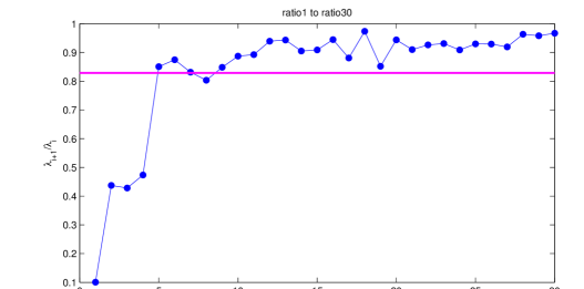
Figure 9: Eigenvalues of $\widehat{M}$

Note

A supplementary file Li et al. [19] collects several technical proofs used in the paper.

Appendix A Supplementary material for the paper “Identifying the number of factors from singular values of a large sample auto-covariance matrix”

This supplementary collects several technical lemmas that are used in the main paper.

Lemma A.1.

$\mathbb{E}(\lambda^{2}I-E_{1}E_{1}^{\prime}E_{2}E_{2}^{\prime})^{-1}E_{1}E_{1}^{\prime}$ and $\mathbb{E}(\lambda^{2}I-E_{2}E_{2}^{\prime}E_{1}E_{1}^{\prime})^{-1}E_{2}E_{2}^{\prime}$ are diagonal.

Lemma A.2.

$\mathbb{E}(\lambda^{2}I-E_{1}E_{1}^{\prime}E_{2}E_{2}^{\prime})^{-1}E_{1}E_{1}^{\prime}E_{2}E_{2}^{\prime}$ and
$\mathbb{E}(\lambda^{2}I-E_{2}E_{2}^{\prime}E_{1}E_{1}^{\prime})^{-1}E_{2}E_{2}^{\prime}E_{1}E_{1}^{\prime}$ are diagonal.

Proof.

The proofs of Lemma A.1 and Lemma A.2 have been already given in the paper [1]. ∎

Lemma A.3.

$$\leavevmode\nobreak\ \leavevmode\nobreak\ \leavevmode\nobreak\ \leavevmode\nobreak\ \mathbb{E}\left[\lambda I_{k}-\lambda X_{1}^{\prime}(\lambda^{2}I-E_{1}E_{1}^{\prime}E_{2}E_{2}^{\prime})^{-1}E_{1}E_{1}^{\prime}X_{1}\right]$$

$$=\mathbb{E}\left[\lambda I_{k}-\lambda X_{0}^{\prime}(\lambda^{2}I-E_{2}E_{2}^{\prime}E_{1}E_{1}^{\prime})^{-1}E_{2}E_{2}^{\prime}X_{0}\right]$$

$$=\begin{pmatrix}\lambda-\frac{\lambda T(\lambda^{2})}{y+T(\lambda^{2})}(1+\gamma_{0}(1))&\cdots&0\\ \vdots&\ddots&\vdots\\ 0&\cdots&\lambda-\frac{\lambda T(\lambda^{2})}{y+T(\lambda^{2})}(1+\gamma_{0}(k))\\ \end{pmatrix}$$

Proof.

$$\leavevmode\nobreak\ \leavevmode\nobreak\ \leavevmode\nobreak\ \leavevmode\nobreak\ \mathbb{E}\left[\lambda I_{k}-\lambda X_{1}^{\prime}(\lambda^{2}I-E_{1}E_{1}^{\prime}E_{2}E_{2}^{\prime})^{-1}E_{1}E_{1}^{\prime}X_{1}\right]$$

$$=\mathbb{E}\left\{\mathbb{E}\left[\lambda I_{k}-\lambda X_{1}^{\prime}(\lambda^{2}I-E_{1}E_{1}^{\prime}E_{2}E_{2}^{\prime})^{-1}E_{1}E_{1}^{\prime}X_{1}\big{|}X_{1}\right]\right\}$$

$$=\mathbb{E}\left\{\lambda I_{k}-\lambda X_{1}^{\prime}E\left[(\lambda^{2}I-E_{1}E_{1}^{\prime}E_{2}E_{2}^{\prime})^{-1}E_{1}E_{1}^{\prime}\right]X_{1}\big{|}X_{1}\right\}\leavevmode\nobreak\ .$$

Since

$$\mathbb{E}\left[(\lambda^{2}I-E_{1}E_{1}^{\prime}E_{2}E_{2}^{\prime})^{-1}E_{1}E_{1}^{\prime}\right]$$

is a diagonal $T\times T$ matrix according to Lemma A.1, and we denote it as

$$diag(d_{1},\cdots,d_{T})\leavevmode\nobreak\ .$$

Then the $(i,i)$-th element of $\mathbb{E}\left\{X_{1}^{\prime}\mathbb{E}\left[(\lambda^{2}I-E_{1}E_{1}^{\prime}E_{2}E_{2}^{\prime})^{-1}E_{1}E_{1}^{\prime}\right]X_{1}\right\}$ equals to

$$\leavevmode\nobreak\ \leavevmode\nobreak\ \mathbb{E}\sum_{j=1}^{T}X_{1}^{\prime}(i,j)d_{j}X_{1}(j,i)=\sum_{j=1}^{T}\mathbb{E}X_{1}^{2}(j,i)d_{j}$$

$$=\frac{1}{T}\sum_{j=1}^{T}\mathbb{E}(x_{i\,j+1}+\varepsilon_{i\,j+1})^{2}\mathbb{E}d_{j}=\frac{1}{T}\sum_{j=1}^{T}(1+\gamma_{0}(i))\mathbb{E}d_{j}$$

$$=\frac{1}{T}(1+\gamma_{0}(i))\mathbb{E}\mathop{\text{tr}}\left[(\lambda^{2}I-E_{1}E_{1}^{\prime}E_{2}E_{2}^{\prime})^{-1}E_{1}E_{1}^{\prime}\right]\leavevmode\nobreak\ ,$$ (A.1)

where the second and third equalities are due to the independence between $x_{t}$ and $\varepsilon_{t}$ and the i.i.d feature of $\varepsilon_{t}$. If we denote

$$x_{T}=\frac{1}{T}tr(E_{1}E_{1}^{\prime}E_{2}E_{2}^{\prime}-\lambda^{2}I)^{-1}\leavevmode\nobreak\ ,$$

$$y_{T}=\frac{1}{T}tr\big{[}(E_{1}E_{1}^{\prime}E_{2}E_{2}^{\prime}-\lambda^{2}I)^{-1}E_{1}E_{1}^{\prime}\big{]}\leavevmode\nobreak\ ,$$

there exists the relationship that:

$$1+\lambda^{2}x_{T}=\frac{y\cdot y_{T}}{1+y_{T}}\leavevmode\nobreak\ ,$$

see (1) in Li et al. [1]. So (A) reduces to:

$$-(1+\gamma_{0}(i))\mathbb{E}y_{T}=-(1+\gamma_{0}(i))\mathbb{E}\left(\frac{1+\lambda^{2}x_{T}}{y-1-\lambda^{2}x_{T}}\right)\leavevmode\nobreak\ .$$ (A.2)

Besides,

$$\mathbb{E}x_{T} =E\left[\frac{1}{T}\mathop{\text{tr}}(E_{1}E_{1}^{\prime}E_{2}E_{2}^{\prime}-\lambda^{2}I)^{-1}\right]$$

$$=\begin{cases}\int_{a}^{b}\frac{1}{x-\lambda^{2}}f(x)dx\leavevmode\nobreak\ ,\leavevmode\nobreak\ \leavevmode\nobreak\ \leavevmode\nobreak\ \leavevmode\nobreak\ y>1\\[8.53581pt] \int_{0}^{b}\frac{1}{x-\lambda^{2}}f(x)dx-\frac{1-y}{\lambda^{2}}\leavevmode\nobreak\ ,\leavevmode\nobreak\ \leavevmode\nobreak\ \leavevmode\nobreak\ \leavevmode\nobreak\ 0<y\leq 1\leavevmode\nobreak\ ,\end{cases}$$

which leads to

$$\mathbb{E}(1+\lambda^{2}x_{T}) =\begin{cases}\int_{a}^{b}\frac{x}{x-\lambda^{2}}f(x)dx\leavevmode\nobreak\ ,\leavevmode\nobreak\ \leavevmode\nobreak\ \leavevmode\nobreak\ \leavevmode\nobreak\ y>1\\[8.53581pt] \int_{0}^{b}\frac{x}{x-\lambda^{2}}f(x)dx\leavevmode\nobreak\ ,\leavevmode\nobreak\ \leavevmode\nobreak\ \leavevmode\nobreak\ \leavevmode\nobreak\ 0<y\leq 1\leavevmode\nobreak\ \end{cases}$$

$$=-T(\lambda^{2})\leavevmode\nobreak\ ,$$

where $f(x)$ is the density function of the LSD of $E_{1}E_{1}^{\prime}E_{2}E_{2}^{\prime}$ (also $E_{2}E_{2}^{\prime}E_{1}E_{1}^{\prime}$), and $T(z)$ is the $T$-transform that associated with $f(x)$ whose support is $[a\cdotp\mathbf{1}_{\{y>1\}},b]$.

Therefore, we have (A.2) equals to

$$(1+\gamma_{0}(i))\frac{T(\lambda^{2})}{y+T(\lambda^{2})}\leavevmode\nobreak\ .$$

For $i\neq k$, the $(i,k)$-th element of

$$\mathbb{E}\left\{X_{1}^{\prime}\mathbb{E}\left[(\lambda^{2}I-E_{1}E_{1}^{\prime}E_{2}E_{2}^{\prime})^{-1}E_{1}E_{1}^{\prime}\right]X_{1}\right\}$$

equals to

$$\mathbb{E}\sum_{j=1}^{T}X_{1}^{\prime}(i,j)d_{j}X_{1}(j,k)=\sum_{j=1}^{T}\mathbb{E}X_{1}(j,i)X_{1}(j,k)\mathbb{E}d_{j}$$

$$= \frac{1}{T}\sum_{i=1}^{T}\mathbb{E}(x_{i\,j+1}+\varepsilon_{i\,j+1})(x_{k\,j+1}+\varepsilon_{k\,j+1})\mathbb{E}d_{j}=0,$$

due to the independence between the coordinates of $x_{t}$ and also the independence between $x_{t}$ and $\varepsilon_{t}$.

All this leads to the fact that

$$\leavevmode\nobreak\ \mathbb{E}\left[\lambda I_{k}-\lambda X_{1}^{\prime}(\lambda^{2}I-E_{1}E_{1}^{\prime}E_{2}E_{2}^{\prime})^{-1}E_{1}E_{1}^{\prime}X_{1}\right]$$

$$=\begin{pmatrix}\lambda-\frac{\lambda T(\lambda^{2})}{y+T(\lambda^{2})}(1+\gamma_{0}(1))&\cdots&0\\ \vdots&\ddots&\vdots\\ 0&\cdots&\lambda-\frac{\lambda T(\lambda^{2})}{y+T(\lambda^{2})}(1+\gamma_{0}(k))\\ \end{pmatrix}\leavevmode\nobreak\ .$$

The same result also holds true for

$$\mathbb{E}\left[\lambda I_{k}-\lambda X_{0}^{\prime}(\lambda^{2}I-E_{2}E_{2}^{\prime}E_{1}E_{1}^{\prime})^{-1}E_{2}E_{2}^{\prime}X_{0}\right]\leavevmode\nobreak\ .$$

The proof of the Lemma is complete.

∎

Lemma A.4.

$$\leavevmode\nobreak\ \mathbb{E}\left[X_{1}^{\prime}\left(I+(\lambda^{2}I-E_{1}E_{1}^{\prime}E_{2}E_{2}^{\prime})^{-1}E_{1}E_{1}^{\prime}E_{2}E_{2}^{\prime}\right)X_{0}\right]$$

$$= \mathbb{E}\left[X_{0}^{\prime}\left(I+(\lambda^{2}I-E_{2}E_{2}^{\prime}E_{1}E_{1}^{\prime})^{-1}E_{2}E_{2}^{\prime}E_{1}E_{1}^{\prime}\right)X_{1}\right]$$

$$= \begin{pmatrix}(1+T(\lambda^{2}))\gamma_{1}(1)&\cdots&0\\ \vdots&\ddots&\vdots\\ 0&\cdots&(1+T(\lambda^{2}))\gamma_{1}(k)\\ \end{pmatrix}$$

Proof.

$$\leavevmode\nobreak\ \mathbb{E}\left[X_{1}^{\prime}\left(I+(\lambda^{2}I-E_{1}E_{1}^{\prime}E_{2}E_{2}^{\prime})^{-1}E_{1}E_{1}^{\prime}E_{2}E_{2}^{\prime}\right)X_{0}\right]$$

$$= \mathbb{E}\left\{\mathbb{E}\left[X_{1}^{\prime}\left(I+(\lambda^{2}I-E_{1}E_{1}^{\prime}E_{2}E_{2}^{\prime})^{-1}E_{1}E_{1}^{\prime}E_{2}E_{2}^{\prime}\right)X_{0}\big{|}X_{0},X_{1}\right]\right\}$$

$$= \mathbb{E}\left\{X_{1}^{\prime}\mathbb{E}\left[I+(\lambda^{2}I-E_{1}E_{1}^{\prime}E_{2}E_{2}^{\prime})^{-1}E_{1}E_{1}^{\prime}E_{2}E_{2}^{\prime}\right]X_{0}\big{|}X_{0},X_{1}\right\}$$

Since

$$\mathbb{E}(\lambda^{2}I-E_{1}E_{1}^{\prime}E_{2}E_{2}^{\prime})^{-1}E_{1}E_{1}^{\prime}E_{2}E_{2}^{\prime}$$

is diagonal according to Lemma A.2, and we denote it as $\text{diag}(a_{1},\cdots,a_{T})$. Then the $(i,i)$-th element of

$$\mathbb{E}\left[X_{1}^{\prime}\left(I+(\lambda^{2}I-E_{1}E_{1}^{\prime}E_{2}E_{2}^{\prime})^{-1}E_{1}E_{1}^{\prime}E_{2}E_{2}^{\prime}\right)X_{0}\right]$$

equals to

$$\leavevmode\nobreak\ \leavevmode\nobreak\ \mathbb{E}\sum_{j=1}^{T}X_{1}^{\prime}(i,j)(1+a_{j})X_{0}(j,i)$$

$$= \sum_{j=1}^{T}\mathbb{E}X_{1}(j,i)X_{0}(j,i)\mathbb{E}(1+a_{j})$$

$$= \frac{1}{T}\sum_{j=1}^{T}\mathbb{E}(x_{i\,j+1}+\varepsilon_{i\,j+1})(x_{i\,j}+\varepsilon_{i\,j})\mathbb{E}(1+a_{j})$$

$$= \frac{1}{T}\sum_{j=1}^{T}\mathbb{E}(x_{i\,j+1}x_{i\,j})\mathbb{E}(1+a_{j})=\frac{1}{T}\sum_{j=1}^{T}\gamma_{1}(i)\mathbb{E}(1+a_{j})$$

$$= \frac{\gamma_{1}(i)}{T}\left(T+\mathbb{E}\mathop{\text{tr}}\left[(\lambda^{2}I-E_{1}E_{1}^{\prime}E_{2}E_{2}^{\prime})^{-1}E_{1}E_{1}^{\prime}E_{2}E_{2}^{\prime}\right]\right)$$

$$= \gamma_{1}(i)\left(1+\int\frac{x}{\lambda^{2}-x}dF(x)\right)=\gamma_{1}(i)(1+T(\lambda^{2}))\leavevmode\nobreak\ .$$

Also for $i\neq k$, the $(i,k)$-th element of

$$\mathbb{E}\left[X_{1}^{\prime}\left(I+(\lambda^{2}I-E_{1}E_{1}^{\prime}E_{2}E_{2}^{\prime})^{-1}E_{1}E_{1}^{\prime}E_{2}E_{2}^{\prime}\right)X_{0}\right]$$

equals to

$$\mathbb{E}\sum_{j=1}^{T}X_{1}^{\prime}(i,j)(1+a_{j})X_{0}(j,k)=\sum_{j=1}^{T}\mathbb{E}X_{1}(j,i)X_{0}(j,k)\mathbb{E}(1+a_{j})$$

$$= \frac{1}{T}\sum_{j=1}^{T}\mathbb{E}(x_{i\,j+1}+\varepsilon_{i\,j+1})(x_{k\,j}+\varepsilon_{k\,j})\mathbb{E}(1+a_{j})=0,$$

where the last equality is due to the independence between the $k$ coordinates of $x_{t}$ and between $x_{t}$ and $\varepsilon_{t}$.

The same is true for

$$\mathbb{E}\left\{\mathbb{E}\left[X_{1}^{\prime}\left(I+(\lambda^{2}I-E_{1}E_{1}^{\prime}E_{2}E_{2}^{\prime})^{-1}E_{1}E_{1}^{\prime}E_{2}E_{2}^{\prime}\right)X_{0}\big{|}X_{0},X_{1}\right]\right\}$$

and we omit the detail.

The proof of this Lemma is complete. ∎

References

- Alessi et al. [2010] Alessi, L., Barigozzi, M. and Capasso, M. (2010) Improved penalization for determining the number of factors in approximate factor models Statist. Probab. Letters 80, 1806-1813.
- Bai and Ng [2002] Bai, J. and Ng, S. (2002). Determining the number of factors in approximate factor models. Econometrica, 70(1), 191-221.
- Bai and Ng [2007] Bai, J. and Ng, S. (2007). Determining the number of primitive shocks in factor models. Journal of Business and Economic Statistics, 25(1), 52-60.
- Bai and Ng [2013] Bai, J. and Ng, S. (2013). Principal components estimation and identification of static factors. J. Econometrics., 176(1), 18–29.
- Bai and Yao [2008] Bai, Z. and Yao, J. (2008). Central limit theorems for eigenvalues in a spiked population model. Ann. Inst. Henri Poincaré Probab. Stat., 44(3), 447–474.
- Bai and Yao [2012] Bai, Z. and Yao, J. (2012). On sample eigenvalues in a generalized spiked population model. J. Multivariate Analysis, 106, 167–177.
- Baik and Silverstein [2006] Baik, J. and Silverstein, J.W. (2006). Eigenvalues of Large Sample Covariance Matrices of Spiked Population Models. J. Multivariate. Anal., 97, 1382–1408.
- Benaych-Georges and Nadakuditi [2011] Benaych-Georges, F. and Nadakuditi, R.R. (2011). The eigenvalues and eigenvectors of finite, low rank perturbations of large random matrices. Adv. Math., 227(2), 494–521.
- Benaych-Georges et al. [2011] Benaych-Georges, F., Guionnet, A. and Maïda, M. (2011). Fluctuations of the extreme eigenvalues of finite rank deformations of random matrices. Electron. J. Probab. 16(60), 1621–1662.
- Forni et al. [2000] Forni, M., Hallin, M., Lippi, M. and Reichlin, L. (2000). The generalized dynamic-factor model: Identification and estimation. Review of Economics and statistics, 82(4), 540-554.
- Forni et al. [2004] Forni, M., Hallin, M., Lippi, M. and Reichlin, L. (2004). The generalized dynamic factor model consistency and rates. J. Econometrics., 119(2), 231-255.
- Forni et al. [2005] Forni, M., Hallin, M., Lippi, M. and Reichlin, L. (2005). The generalized dynamic factor model: one sided estimation and forecasting. J. Amer. Statist. Assoc., 100, 830-840.
- Geweke [1977] Geweke J. (1977). The dynamic factor analysis of economic time series. in Latent variables in Socio-Economic Models, ed. by D.J.Aigner and A.S.Goldberger, Amsterdam:North-Holland.
- Hallin and Liska [2007] Hallin, M. and Liska, R. (2007). Determining the number of factors in the general dynamic factor model. J. Amer. Statist. Assoc., 102(478), 603-617.
- Jin et al. [2014] Jin, B., Wang, C., Bai, Z., Nair, K. and Harding, M. (2014) Limiting spectral distribution of a symmetrized auto-cross covariance matrix. Ann. Applied Probab. 24(3), 1199-1225.
- Johnstone [2001] Johnstone, I. (2001). On the distribution of the largest eigenvalue in principal components analysis. Ann. Statistics, 29(2), 295–327.
- Lam and Yao [2012] Lam, C. and Yao, Q.W. (2012). Factor modeling for high-dimensional time series: inference for the number of factors. Ann. Statist. 40, 694-726.
- Li et al. [2014] Li, Z., Pan, G.M. and Yao, J. (2014). On singular value distribution of large-dimensional autocovariance matrices. Preprint (arxiv:1402.6149).
- Li et al. [2014] Li, Z., Wang, Q.W. and Yao, J. (2014). In Appendix of this paper: “Supplementary material for the paper “Identifying the number of factors from singular values of a large sample auto-covariance matrix”.
- Onatski [2010] Onatski, A. (2010). Determining the number of factors from empirical distribution of eigenvalues. The Review of Economics and Statistics, 92(4), 1004-1016.
- Onatski [2012] Onatski, A. (2012) Asymptotics of the principal components estimator of large factor models with weakly influential factors. J. Econometrics 168 (2), 244-258.
- Onatski [2015] Onatski, A. (2015) Asymptotic analysis of the squared estimation error in misspecified factor models. J. Econometrics 186 (2), 388-406.
- Passemier and Yao [2012] Passemier, D. and Yao, J. (2012). On determining the number of spikes in a high-dimensional spiked population model. Random Matrices: Theory and Applications, 1, 1150002.
- Sargent and Sims [1977] Sargent, T. J. and Sims, C. A. (1977). Business cycle modeling without pretending to have too much a priori economic theory. New methods in business cycle research, 1, 145-168.
- Stock and Watson [2011] Stock, J. H. and Watson, M W. (2011). Dynamic factor models. Oxford Handbook of Economic Forecasting, 1, 35-59.
- Wang et al. [2015] Wang, C., Jin, B., Bai, Z., Nair, K. and Harding, M. (2015) Strong limit of the extreme eigenvalues of a symmetrized auto-cross covariance matrix. Forthcoming in Ann. Applied. Probab. (http://www.imstat.org/aap/future_papers.html)
- Wang and Yao [2014] Wang, Q. W. and Yao, J. (2014). Moment approach to for singular values distribution of a large auto-covariance matrix. Preprint (arxiv:1410.0752).

References

- Li et al. [2014] Li, Z., Pan, G.M. and Yao, J. (2014). On singular value distribution of large-dimensional autocovariance matrices. Preprint (arxiv:1402.6149).