Greedy Sparsity–Promoting Algorithms for Distributed Learning

Abstract

This paper focuses on the development of novel greedy techniques for distributed learning under sparsity constraints. Greedy techniques have widely been used in centralized systems due to their low computational requirements and at the same time their relatively good performance in estimating sparse parameter vectors/signals. The paper reports two new algorithms in the context of sparsity–aware learning. In both cases, the goal is first to identify the support set of the unknown signal and then to estimate the non–zero values restricted to the active support set. First, an iterative greedy multi–step procedure is developed, based on a neighborhood cooperation strategy, using batch processing on the observed data. Next, an extension of the algorithm to the online setting, based on the diffusion LMS rationale for adaptivity, is derived. Theoretical analysis of the algorithms is provided, where it is shown that the batch algorithm converges to the unknown vector if a Restricted Isometry Property (RIP) holds. Moreover, the online version converges in the mean to the solution vector under some general assumptions. Finally, the proposed schemes are tested against recently developed sparsity–promoting algorithms and their enhanced performance is verified via simulation examples.

I Introduction

Many real–life signals and systems can be described by parsimonious models consisting of few non–zero coefficients. Typical examples include: image and video signals, acoustic signals, echo cancellation, wireless multipath channels, High Definition TV, just to name but a few, e.g., [1, 2, 3, 4, 5, 6]. This feature is of particular importance under the big data paradigm and the three associated dimensions (Volume, Velocity, Variety) [7], where the resulting data set can not be processed as is and exploitation of significant variables becomes crucial. The goal of this paper is to develop sparsity–promoting algorithms for the estimation of sparse signals and systems in the context of distributed environments. It is anticipated that sparsity–aware learning will constitute a major pillar for big data analytics, which currently seek for decentralized processing and fast execution times [7, 8].

Two of the main paths for developing schemes for sparsity–aware learning, are a) regularization of the cost via the $\ell_{1}$ norm of the parameter vector (Basis pursuit), e.g., [9, 2], and b) via the use of greedy algorithms (or Matching Pursuit) [10, 11, 12, 13, 14, 15, 16, 17]. In the greedy schemes, the support set, in which the non–zero coefficients lie is first identified and then the respective coefficients are estimated in a step–wise manner. Each one of the above algorithmic families poses their own advantages and disadvantages. The $\ell_{1}$–regularization methods provide well established recovery conditions, albeit at the expense of longer execution times and offline fine tuning. On the contrary, greedy algorithms perform at lower computational demands; moreover, they still enjoy theoretical justifications for their performance, under some assumptions.

With only few exceptions, e.g., [18, 19, 20, 21, 22, 23], sparsity promoting algorithms assume that the training data, through which the unknown target vector is estimated, are centrally available. That is, there exist a central processing unit (or Fusion Center, FC), which has access to all training data, and performs all essential computations. Nevertheless, in many applications the need for decentralized/distributed processing rises. Typical examples of such applications are those involving wireless sensor networks (WSNs), which are deployed over a geographical region or software agents monitoring software operations over a network to diagnose and prevent security threats, and the nodes are tasked to collaboratively estimate an unknown (but common) sparse vector. The existence of a fusion center, which collects all training data and then performs the required computations, may be prohibited due to geographical constraints and/or energy and bandwidth limitations. Furthermore, in many cases, e.g., medical applications, privacy has to be preserved which means that the nodes are not allowed to exchange their learning data but only their learning results [24]. Hence, the development of distributed algorithms is of significant importance.

This paper is concerned with the task of sparsity–aware learning, via the greedy avenue, by considering both batch as well as online schemes. In the former, it is assumed that each node possesses a finite number of input/output measurements, which are related via the unknown sparse vector. The support set is computed in a collaborative way; that is, the nodes exchange their measurements and exploit them properly so as to identify the positions of the non–zero coefficients. In the sequel, the produced estimates, which are restricted to the support set, are fused according to a predefined rule. The online scenario deals with an infinite number of observations, received sequentially at each node. In general, adaptive/online algorithms update the estimates of the unknown vector dynamically, in contrast to their batch counterparts, where for every new pair of data, estimation of the unknown vector is repeated from scratch. Such techniques can handle cases where the unknown signal and its corresponding support set is time–varying and also cases where the number of available data is very large and the computational resources are not enough for such handling. In the greedy–based adaptive algorithm, which is proposed here, the nodes cooperate in order to estimate their support sets, and the diffusion rationale, e.g., [25], is adopted for the unknown vector estimation.

The paper is organized as follows. In Section II, the problem formulation is described. In Section III the distributed greedy learning problem is discussed and the batch learning algorithm is provided. Section IV presents the adaptive distributed learning problem, together with the proposed adaptive scheme and in Section V the theoretical properties of the presented algorithms are discussed. Finally, in Section VI, the performance of the proposed algorithmic schemes is validated. Details of the derivations are given in the appendices.

Notation: The set of all non–negative integers and the set of all real numbers will be denoted by ${\mathbb{Z}}$ and ${\mathbb{R}}$ respectively. Vectors and matrices will be denoted by boldface letters and uppercase boldface letters respectively. The Euclidean norm will be denoted by $\|\cdot\|_{\ell_{2}}$ and the $\ell_{1}$ norm by $\|\cdot\|_{\ell_{1}}$. Given a vector $\bm{h}\in{\mathbb{R}}^{m}$, the operator $\mathrm{supp}_{s}(\bm{h})$ returns the subset of the $s$ largest in magnitude coefficients. Moreover, $\mathbb{E}[\cdot]$ stands for the expectation operator. Finally, $|\mathcal{S}|$ denotes the cardinality of the set $\mathcal{S}$.

II Problem Formulation

Our task is to estimate an unknown sparse parameter vector, $\bm{h}_{*}\in{\mathbb{R}}^{m}$, exploiting measurements, collected at the $N$ nodes of an ad–hoc network, under a preselected cooperative protocol. The greedy philosophy will be employed. Such a network is illustrated in Fig. 1. We denote the node set by ${\mathcal{N}}=\{1,\ldots,N\}$, and we assume that each node is able to exchange information with a subset of ${\mathcal{N}}$, namely ${\mathcal{N}}_{k}\subseteq{\mathcal{N}},k=1,\ldots,N$. This set is also known as the neighborhood of $k$. The input–output relation adheres to the following linear model:

$$\bm{y}_{k}=\bm{A}_{k}\bm{h}_{*}+\bm{\eta}_{k},\ \forall k\in{\mathcal{N}},$$ (1)

where $\bm{A}_{k}$ is an $l\times m$ sensing matrix, with $l<m$, $\bm{y}_{k}\in{\mathbb{R}}^{l}$ and $\bm{\eta}_{k}\in{\mathbb{R}}^{l}$ is an additive white noise process. The vector to be estimated is assumed to be at most $s$–sparse, i.e., $\|\bm{h}_{*}\|_{\ell_{0}}\leq s\ll m$, where $\|\cdot\|_{\ell_{0}}$ denotes the $\ell_{0}$ (pseudo) norm.

Figure 1: An ad–hoc network. 

II-A Sparsity–Aware Distributed Learning: The DLasso Algorithm

A version of the celebrated Lasso algorithm, in the context of distributed learning, is the so–called Distributed Lasso (DLasso) algorithm, proposed in [18]. This algorithm solves the following problem:

$$\hat{\bm{h}}=\arg\min_{\|\bm{h}\|_{\ell_{1}}\leq\delta}\sum_{k\in{\mathcal{N}}}\|\bm{y}_{k}-\bm{A}_{k}\bm{h}\|_{\ell_{2}}^{2}.$$ (2)

This optimization can be reformulated in a fully decentralized way, where each node exploits local information, as well as information received by the neighborhood. The decentralized optimization can be efficiently solved by adopting the Alternating Direction–Method of Multipliers (ADMM), [26]. It has been shown in [18], that the solution of the decentralized task where each node has access to locally obtained observations as well as estimates collected by its neighborhood, coincides with the solution obtained by solving (2), which requires global information. It should be pointed out that each node lacks global network information; however, if an appropriate cooperation protocol is adopted, then the global solution can be obtained. The adopted cooperation protocol, which is based on the ADMM and can assure such a behaviour, is known as consensus protocol and constitutes the beginning for several distributed learning algorithms, e.g., the distributed Support Vector Machines, [27], etc.

III Distributed greedy learning

Greedy algorithms, e.g., [10, 11, 12, 13, 14, 15, 16, 6], offer an alternative sparsity-promoting route to $\ell_{1}$–regularization; our goal is to extend the philosophy behind such algorithms in the framework of distributed learning.

Under the centralized scenario, greedy techniques iteratively estimate the unknown parameter by applying the following two–step approach:

• Subset Selection: First, a proxy signal is computed (which carries information regarding the support set of the unknown vector) based on input–output measurements. In the sequel, the $s$ largest in amplitude coefficients of the proxy are computed.

• Greedy Update: The estimate of the unknown vector is computed, by performing a Least–Squares task restricted to the identified support set.

To keep the discussion simple, let us assume that the signal proxy is computed in an non–cooperative way; that is, each node exploits solely its locally obtained measurements. Following the rationale of the majority of greedy algorithms (see, for example, [10, 11, 12, 13, 14, 15, 16]) decisions concerning the support set should be based on a signal proxy of the form

$$\bm{A}_{k}^{T}\left(\bm{y}_{k}-\bm{A}_{k}\widehat{\bm{h}}_{k}\right)\approx\bm{A}_{k}^{T}\bm{A}_{k}\left({\bm{h}}_{*}-\widehat{\bm{h}}_{k}\right),$$

where $\widehat{\bm{h}}_{k}$ stands for the estimate of ${\bm{h}}_{*}$ obtained at note $k$. It is important to note that for such a proxy, the algorithm at every iteration, selects distinct indices. Since the vast majority of greedy algorithm are iterative and hence it is important not to consider indices that have been previously picked. This is ensured by orthogonalizing the residual. An enhanced proxy, which would allow multiple selection of indices, has the following form:

$$\mathrm{supp}_{s\text{ or }2s}\left(\bm{A}_{k}^{{\color[rgb]{0,0,0}T}}\left(\bm{y}_{k}-\bm{A}_{k}\widehat{\bm{h}}_{k}\right)\right)\cup\mathrm{supp}_{s}\left(\widehat{\bm{h}}_{k}\right),$$

and in such cases, the estimation step is restricted to a set of indices larger than $s$. However, adopting such philosophies for the proxy signals in distributed learning leads to problems. In distributed learning, the only quantity, which commonly affects all nodes, is the true vector ${\bm{h}}_{*}$ (This can be readily seen from (1)). Both previously mentioned proxy signals carry time–varying information from local estimates, which are different from node to node, and hence may pose problems to the support set consensus, i.e., the nodes’ “agreement” to the same support set. Thus, it is preferable to find a proxy which is close to ${\bm{h}}_{*}$ instead of $\left({\bm{h}}_{*}-\widehat{\bm{h}}_{k}\right)$. This is an important point for our analysis to follow, since such a mechanism will lead to the required consensus among the nodes.

To this direction, we adopt a similar methodology to the one presented in [28], which selects the $s$ dominant coefficients of the following proxy:

$$\hat{\bm{h}}_{k}+\bm{A}_{k}^{T}(\bm{y}_{k}-\bm{A}_{k}\hat{\bm{h}}_{k})\approx\bm{h}_{*}.$$ (3)

The intuition of this proxy selection is that the left hand side (lhs) of (3) is a gradient descent iteration using the measurements $\bm{A}_{k},\ \bm{y}_{k}$. It has been verified experimentally (see for example [28] for the centralized case) that a few iterations are enough to recover the support under a certain condition on the restricted isometry constant.

In decentralized/distributed learning, the subset selection and greedy update steps can be further enriched by exploiting the information that is available at the nodes of the network. Recall that, each node is able to communicate and exchange data with the neighboring nodes, where a direct link is available. Hence, the signal proxies can be computed in a cooperative fashion and instead of exploiting only local quantities of interest, spatially received data will take part in the support set identification. As it will become clear in the simulations section, this turns out to be beneficial to the performance of the proposed algorithms.

In the sequel, we present a unified method for sparsity–aware distributed learning, adopting the greedy viewpoint. The core steps, through which the algorithms for batch and adaptive learning “spring”, are summarized below:

• Information Enhancement for Subset Selection: Each node exchanges information with its neighbours, in order to construct the signal proxy, instead of relying only on its local measurements.

• Cooperative Estimation Restricted on the Support Set: At each node, a Least Squares is performed restricted on the support sets that were computed cooperatively in the previous step. The neighbourhood exchanges their estimates and fuse them under a certain protocol.

• Pruning Step: Neighbouring nodes may have identified different support sets, due to the dissimilarity of their measurements. Hence, the result of the previously mentioned fusion may not give an $s$–sparse estimate. To this end, pruning ensures that, at each iteration, an $s$–sparse vector is produced.

Before we proceed any further, let us explain the basic principles that underlie the cooperation among the nodes. Each node, at each iteration step, fuses under a certain rule the estimates and/or the measurements, which are received from the neighbourhood. This fusion is dictated by the combination coefficients, which obey the following rules: $a_{r,k}>0$, if $r\in{\mathcal{N}}_{k}$, $a_{r,k}=0$, if $r\notin{\mathcal{N}}_{k}$ and $\sum_{r\in{\mathcal{N}}_{k}}a_{r,k}=1,\forall k\in{\mathcal{N}}$. Furthermore, it is assumed that each node is a neighbor of itself, i.e., $a_{k,k}>0,\ \forall k\in\mathcal{N}$. In words, every node assigns a weight to the estimates and/or measurements of the neighborhood and a convex combination of them is computed; the resulting aggregate is used properly in the learning scheme. Two well known examples of combination coefficients are: a) the Metropolis rule, where

$$a_{r,k}=\begin{cases}\frac{1}{\mathrm{max}\left\{|{\mathcal{N}}_{k}|,|{\mathcal{N}}_{r}|\right\}},&\text{if $r\in{\mathcal{N}}_{k}$ and $r\neq k$},\\ 1-\sum_{r\in{\mathcal{N}}_{k}\setminus k}a_{r,k},&\text{if $r=k$},\\ 0,&\mathrm{otherwise},\end{cases}$$

and b) the uniform rule, in which:

$$a_{r,k}=\begin{cases}\frac{1}{|{\mathcal{N}}_{k}|},&\text{if $r\in{\mathcal{N}}_{k}$},\\ 0,&\mathrm{otherwise}.\end{cases}$$

III-A Batch Mode Learning via the DiHaT algorithm

In this section, a batch parsity-promoting algorithm, which we will call Distributed Hard Thresholding Pursuit Algorithm (DiHaT), is presented. The algorithmic steps are summarized in Table I.

TABLE I: The Distributed Hard Thresholding Algorithm (DiHaT)

Algorithm description			Complexity
$\bm{h}_{k,0}=\bm{0}_{m},\quad\overline{\bm{y}}_{k,0}=\bm{y}_{k},\quad\overline{\bm{A}}_{k,0}=\bm{A}_{k},\quad\mathcal{S}_{k,0}=\emptyset,\quad\mathrm{sparsity\ level}\ \ \ s$		{Initialization}
Loop
1:	$\overline{\bm{y}}_{k,n}=\sum\limits_{r\in\mathcal{N}_{k}}a_{r,k}\overline{\bm{y}}_{r,n-1}$	{Combine local output measurements}	$\mathcal{O}(|{\mathcal{N}}_{k}|l)$
2:	$\overline{\bm{A}}_{k,n}=\sum\limits_{r\in\mathcal{N}_{k}}a_{r,k}\overline{\bm{A}}_{r,n-1}$	{Combine local input measurements}	$\mathcal{O}(|{\mathcal{N}}_{k}|ml)$
3:	${\mathcal{S}}_{k,n}=\mathrm{supp}_{s}\left(\bm{h}_{k,n-1}+\overline{\bm{A}}_{k,n}^{T}(\overline{\bm{y}}_{k,n}-\overline{\bm{A}}_{k,n}\bm{h}_{k,n-1})\right)$	{Identify $s$ largest components}	$\mathcal{O}(ml^{2})$
4:	$\hat{\bm{h}}_{k,n}=\arg\min_{\bm{h}}\left\{\|\overline{\bm{y}}_{k,n}-\overline{\bm{A}}_{k,n}\bm{h}\|_{\ell_{2}}^{2}\right\},\mathrm{supp}(\bm{h})\subset{\mathcal{S}}_{k,n}$	{Signal Estimation}	$\mathcal{O}(m^{2}l)$
5:	$\tilde{\bm{h}}_{k,n}=\sum\limits_{r\in\mathcal{N}_{k}}b_{r,k}\hat{\bm{h}}_{r,n}$	{Combine local estimates}	$\mathcal{O}(|{\mathcal{N}}_{k}|m)$
6:	${\bm{h}}_{k,n}=\mathrm{supp}_{s}(\tilde{\bm{h}}_{k,n})$	{Identify $s$ largest components}	$\mathcal{O}(m)$
Until halting condition is true

In steps 1 and 2 of Table I, the nodes exchange their input–output measurements and fuse them under a certain protocol. This information fusion is dictated by the combination weights $a_{r,k},\ \forall k\in{\mathcal{N}},\ \forall l\in{\mathcal{N}}_{k}$. It is shown later, that if these coefficients are chosen properly, then $\overline{\bm{A}}_{k,n}$ and $\overline{\bm{y}}_{k,n}$ tend asymptotically to the average values, i.e., $\frac{1}{N}\sum_{r=1}^{N}\bm{A}_{r}$ and $\frac{1}{N}\sum_{r=1}^{N}\bm{y}_{r},$ respectively. This improves significantly the performance of the algorithm, since as the number of iteration increases, the information related to the support set is accumulated, in the sense that the support set identification and the parameter estimation procedure will contain information which comes from the entire network. In step 3, the $s$ largest in amplitude coefficients of the signal proxy are selected, and step 4 performs a Least–Squares operation restricted on the support set, which is computed in the previous step. Next (step 5), the nodes exchange their estimates and fuse them in a similar way as in steps 1, 2. Notice that, the combination coefficients may be different from the weights used in input/output measurement combination (denoted as $b_{r,k}$). Finally, since the nodes have access to different observations, especially in the first iterations in which their input–output data are not close to the average values, the estimated support sets among the neighborhood may be different. This implies that in step 5 there is no guarantee that the produced estimate will be $s$–sparse. For this reason, in step 6, a thresholding operation takes place and the final estimate at each node is $s$–sparse. A proof concerning the convergence of the DiHaT algorithm can be found in Section V.

Remark 1

The DiHaT algorithm requires the transmission of $m\times l,l,m$ coefficients from each node, coming from the input matrix, the output and the estimate, respectively. There are two working scenarios to relax the required bandwidth for such an exchange. The exchange of the information takes place in blocks, in line with the available bandwidth constraints. Since this is a batch processing mode of operation, such a scenario will slow down the overall execution time, and has no effect on processing/memory resources. The alternative scenario is to transmit only the obtained estimated, which amounts to $m$ coefficients per iteration step; as simulation show this amounts to a small performance degradation.

IV THE ONLINE LEARNING SETUP

This section deals with an online learning version for the solution of the task. More specifically, our goal is to estimate a sparse unknown vector, ${\bm{h}}_{*}\in{\mathbb{R}}^{m}$, exploiting an infinite number of sequentially arriving measurements collected at the $N$ nodes of an ad–hoc network e.g., [29, 30, 6]. Each node $k$, at each (discrete) time instant, has access to the measurement pair $(y_{k}(n),{\bm{a}}_{k}(n))\in{\mathbb{R}}\times{\mathbb{R}}^{m}$, which are related via the linear model:

$$y_{k}(n)={\bm{a}}_{k}^{T}(n){\bm{h}}_{*}+v_{k}(n),\ \forall k\in{\mathcal{N}},\ \forall n\in{\mathbb{Z}},$$ (4)

where the term $v_{k}(n)$ stands for the additive noise process at each node.

In the literature, for the adaptive distributed learning task, the following modes of cooperation have been proposed:

1. Adapt Then Combine (ATC) [30]: In this strategy, each node computes an intermediate estimate by exploiting locally sensed measurements. After this step, each network agent receives these estimates from the neighbouring nodes and combines them, in order to produce the final estimate.

2. Combine Then Adapt (CTA) [29, 31]: Here, the combination step precedes the adaptation one.

3. ADMM Based [32]: In this category, the computations are made in parallel and there is no clear distinction between the combine and the adapt steps.

The ATC and the CTA cooperation strategies belong to the family of the diffusion–based algorithms. In these schemes, the cooperation among the nodes can be summarized as follows: each node receives estimates from the neighbourhood, and then takes a convex combination of them. In this paper, the ATC strategy is followed, since it has been verified that it converges faster to a lower steady state error floor compared to the other methodologies [33].

IV-A Greedy–Based Adaptive Distributed Learning

Our goal here is to reformulate properly the distributed greedy steps, which are described in Section III, so as to employ them in an adaptive scenario. For simplicity, let us first discuss the non–cooperative case. In the batch learning setting, the proxy signal is constructed via the available measurements at each node; i.e., the local measurements and the information received from the neighbourhood. As we have already described, in online learning the observations are received sequentially, one per each time step and, consequently, a different route has to be followed. Recall the definition of the signal proxy, given in (3). A first approach is to make the following substitutions $\bm{A}_{k}^{T}\bm{y}_{k}$ with $\bm{a}_{k}(n)y_{k}(n)$ and $\bm{A}_{k}^{T}\bm{A}_{k}$ with $\bm{a}_{k}(n)\bm{a}_{k}^{T}(n)$. A drawback of this choice is that the proxy is constructed exploiting just a single pair of data, which in practice carries insufficient information. Another viewpoint, which is followed here, is to rely on approximations of the expected value of the previous quantities, i.e., $\mathbb{E}[\bm{a}_{k}(n)y_{k}(n)]$, $\mathbb{E}[\bm{a}_{k}(n)\bm{a}_{k}^{T}(n)]$. Since the statistics are usually unknown and might exhibit time–variations, we rely on the following approximations, $\mathbb{E}[\bm{a}_{k}(n)y_{k}(n)]\approx\sum_{i=1}^{n}\zeta^{n-i}\bm{a}_{k}(i)y_{k}(i)$, $\mathbb{E}[\bm{a}_{k}(n)\bm{a}_{k}^{T}(n)]\approx\sum_{i=1}^{n}\zeta^{n-i}\bm{a}_{k}(i)\bm{a}_{k}^{T}(i)$, where $\zeta\in(0,1]$ is the so–called forgetting factor, incorporated in order to give less weight to past values.

The modified proxy, which is suitable for adaptive operation takes the following form:

$$\bm{h}_{k}(n-1)+\tilde{\mu}_{k}(\overline{\bm{p}}_{k}(n)-\overline{\bm{R}}_{k}(n)\bm{h}_{k}(n-1))\approx{\bm{h}}_{*},$$ (5)

where $\bm{h}_{k}(n-1),\ \overline{\bm{p}}_{k}(n)$ and $\overline{\bm{R}}_{k}(n)$ are defined in Table II and is $\tilde{\mu}_{k}$ the step size. The proposed proxy constitutes a distributed exponentially weighted extension of its centralized form (addressed in [28]). Notice that (5) defines a gradient descent iteration using the approximate statistics $\overline{\bm{p}}_{k}(n)$ and $\overline{\bm{R}}_{k}(n)$. Assuming that we have at our disposal the true statistical values, i.e., $\overline{\bm{p}}_{k}:=\sum_{r\in{\mathcal{N}}_{k}}a_{r,k}{\bm{p}}_{r}$ and $\overline{\bm{R}}_{k}:=\sum_{r\in{\mathcal{N}}_{k}}a_{r,k}{\bm{R}}_{r}$, then the recursion (5) converges to the true solution, e.g., [25]. In practice, we use the previously mentioned approximate values, since we do not have access to the true statistics; as it will be become apparent in the simulations section, adopting such an approximation has little effect on the comparative performance of the algorithm.

TABLE II: The Greedy Diffusion LMS Algorithm

Algorithm description			Complexity
$\bm{h}_{k}(0)=0,\bm{p}_{k}(0)=0,\bm{R}_{k}(0)=0$		{Initialization}
$0<\zeta\leq 1$		{Forgetting factor}
$0<D$		{Threshold for proxy selection}
For $n:=1,2,\ldots$ do
1:	$\bm{p}_{k}(n)=\frac{n}{n+1}\zeta\bm{p}_{k}(n-1)+\frac{\bm{a}_{k}(n)y_{k}(n)}{n+1}$	{Form cross-correlation}	$O(m)$
2:	$\overline{\bm{p}}_{k}(n)=\sum\limits_{l\in\mathcal{N}_{k}}b_{l,k}\bm{p}_{l}(n)$	{Combine cross–correlation}	$O(|\mathcal{N}_{k}|m)$
3:	$\bm{R}_{k}(n)=\frac{n}{n+1}\zeta\bm{R}_{k}(n-1)+\frac{\bm{a}_{k}(n)\bm{a}_{k}^{T}(n)}{n+1}$	{Form autocorrelation}	$O(m^{2})$
4:	$\overline{\bm{R}}_{k}(n)=\sum\limits_{l\in\mathcal{N}_{k}}b_{l,k}\bm{R}_{l}(n)$	{Combine autocorrelation}	$O(|\mathcal{N}_{k}|m^{2})$
If  $\|\bm{h}_{k}(n-1)\|_{\ell_{2}}\leq D$
5:	$\begin{aligned} \widehat{\bm{S}}_{k,n}&=\mathrm{supp}_{s}\Big{(}\bm{h}_{k}(n-1)+\tilde{\mu}_{k}\Big{(}\overline{\bm{p}}_{k}(n)\\ &-\overline{\bm{R}}_{k}(n)\bm{h}_{k}(n-1)\Big{)}\Big{)}\end{aligned}$	{Identify large components}	$O(m)$
Else
6:	$\begin{aligned} \widehat{\bm{S}}_{k,n}&=\mathrm{supp}_{s}\Big{(}\frac{\bm{h}_{k}(n-1)}{\|\bm{h}_{k}(n-1)\|_{\ell_{2}}}+\tilde{\mu}_{k}(\overline{\bm{p}}_{k}(n)\\ &-\overline{\bm{R}}_{k}(n)\frac{\bm{h}_{k}(n-1)}{\|\bm{h}_{k}(n-1)\|_{\ell_{2}}})\Big{)}\end{aligned}$	{Identify large components}	$O(m)$
7:	$\begin{aligned} \bm{\psi}_{k}(n)&=\bm{h}_{k|\widehat{\mathcal{S}}_{k,n}}(n-1)+\\ &\mu_{k}\bm{a}_{k|\widehat{\mathcal{S}}_{k,n}}(n)[y_{k}(n)-\bm{a}_{k|\widehat{\mathcal{S}}_{k,n}}^{T}(n)\bm{h}_{k|\widehat{\mathcal{S}}_{k,n}}(n-1)]\end{aligned}$	{LMS iteration}	$O(s)$
8:	$\widetilde{\bm{h}}_{k}(n)=\sum\limits_{r\in\mathcal{N}_{k}}c_{r,k}\bm{\psi}_{r|\widehat{\mathcal{S}}_{l,n}}(n)$	{Combine local estimates}	$O(|\mathcal{N}_{k}|s)$
9:	$\widetilde{\mathcal{S}}_{k,n}=\mathrm{supp}_{s}\left(\widetilde{\bm{h}}_{k}(n)\right),\ \bm{h}_{k|\widetilde{\mathcal{S}}^{c}_{k,n}}(n)=\bm{0}$	{Obtain the pruned support}	$O(m)$

Table II summarizes the core steps of the proposed Greedy Diffusion LMS (GreeDi–LMS). Steps 1–5 constitute the distributed greedy subset selection process. It is worth pointing out that the Steps 1–4 create, in a cooperative manner, the basic elements needed for the proxy update and Steps 5–6 select the $s$–largest components. Notice that $D$ is a sufficiently large parameter, which is used to normalize the estimate in the proxy computation step, if its norm is larger than this threshold, and it is employed so as to prevent the proxy from taking extensively large values. It should be pointed out that the distributed greedy update is established via the Adapt–Combine LMS (Steps 7 & 8) of [30]. The diffusion Steps 2, 4 and 8 bring the local estimates closer to the global estimates based on the entire network [30]. Finally, because we are operating in a network of different nodes, some of them will achieve support set convergence faster than others. Therefore, at a node level, we pay more attention to the $s$–dominant positions via the introduction of a pruning step directly after the adaptation in the combined greedy update (Step 9).

Remark 2

The computational complexity of GreeDi–LMS is linear except from the update of $\bm{R}_{k}(n)$, which requires $\mathcal{O}(m^{2})$ operations per iteration. However, exploitation of the shift structure in the regressor vector allows us to drop the computational cost to $\mathcal{O}(m)$, e.g., [34]. Complexity as well as the number of transmitted coefficients, can be decreased if in steps 5 and 6 each node exploits only local information. Regarding the communication cost of the proposed algorithms, each node transmits, overall $2*m+m^{2}$ values corresponding the estimation vector, the crosscorrelation vector and the autocorrelation matrix. However, this cost can be significantly decreased if one exploits the shift structure of the regression vectors. More precisely, in that case, instead of the $m^{2}$ entries of the autocorrelation matrix, only $2m$ coefficients need to be exchanged due to the Teoplitz structure of the autocorrelation matrix, [34, 6]. Finally, another way to bypass the need for transmission of the autocorrelation matrices and the crosscorrelation vectors is to compute them at node level. In particular, according to this scenario, each node receives from the neighborhood the input/output data and computes the respective quantities. Employing this methodology reduces the communication cost to $2m+1$ coefficients, which correspond to the estimate and input vectors and the output. This comes at the cost of an increased complexity.

Remark 3

Another way to reduce complexity is by updating the gradient part of the proxy recursively, as it was done in [35] for the centralized case. However, such an update, although it is computationally lighter, it results in slower support convergence, since the resulting exponentially weighted average contains all $\bm{h}_{k}(t),t:=1,\ldots,n-1$ and not only the current estimate.

V Convergence Analysis

In this section, the theoretical properties of the proposed schemes are studied. In a nutshell, we show that the DiHaT scheme converges, under certain assumptions regarding the noise vectors and a restricted isometry constant for the average value of the input matrices. Regarding the GreeDi–LMS we prove that the algorithm is unbiased, i.e., it converges in the mean to the true unknown vector. Finally, steady–state error bounds are provided.

V-A Convergence Analysis: The Batch Mode Learning Case

The assumptions on the network and associated weights that are needed to establish convergence of the proposed algorithm are given next.

Assumptions 1

Let us define the $N\times N$ matrix $\bm{W}_{1}$, the coefficients formed by the combination weights $a_{r,k}$. This matrix satisfies the following assumptions:

1. $\bm{1}_{N}^{T}\bm{W}_{1}=\bm{1}_{N}^{T}$, where $\bm{1}_{N}\in{\mathbb{R}}^{N}$ is the vector of ones.

2. $\bm{W}_{1}\bm{1}_{N}=\bm{1}_{N}$.

3. $\lambda(\bm{W}_{1}-\bm{1}_{N}\bm{1}_{N}^{T}/N)<1$, where $\lambda(\cdot)$ stands for the maximum eigenvalue of the respective matrix, e.g., [36].

The same assumptions hold for $\bm{W}_{2}$, with entries $b_{r,k}$. Such assumptions are widely employed in distributed learning, e.g., [25, 36]. Methods for constructing the combination matrix, so as to fulfil these assumptions in a decentralized fashion, have been proposed, e.g., [36].
Fact: [36] Under the above assumptions the following hold

$$\lim_{n\rightarrow\infty}\overline{\bm{y}}_{k,n}=\overline{\bm{y}}:=\frac{1}{N}\sum_{r=1}^{N}\bm{y}_{r},\ \forall k\in{\mathcal{N}},$$ (6)

as well as

$$\lim_{n\rightarrow\infty}\overline{\bm{A}}_{k,n}=\overline{\bm{A}}:=\frac{1}{N}\sum_{r=1}^{N}\bm{A}_{r},\ \forall k\in{\mathcal{N}}.$$ (7)

The network nodes, asymptotically, gain access to the mean value of the measurement matrix and measurement vector by reaching consensus.

Assumptions 2

1. The noise terms $\bm{\eta}_{k}$ are assumed to be zero mean and of bounded variance. A typical example is the Gaussian distribution. Moreover, they are spatially independent over the nodes.

2. For a large value of $n$, say $n_{0}$, we assume that

   $$\overline{\bm{y}}_{k,n}\approx\frac{1}{N}\sum_{r=1}^{N}{\bm{A}}_{r}\bm{h}_{*}+\frac{1}{N}\sum_{r=1}^{N}\bm{\eta}_{r}\approx\overline{\bm{A}}\bm{h}_{*},\ \forall n\geq n_{0}.$$

   This is a direct consequence of the fact, that if the combination coefficients are chosen with respect to Assumptions 1.1-1.3, then $\lim_{n\rightarrow\infty}\overline{\bm{y}}_{k,n}=\frac{1}{N}\sum_{r=1}^{N}\bm{y}_{r},\ \forall k\in{\mathcal{N}}$ and $\lim_{n\rightarrow\infty}\overline{\bm{A}}_{k,n}=\frac{1}{N}\sum_{r=1}^{N}\bm{A}_{r},\ \forall k\in{\mathcal{N}}$.

   In other words, for sufficiently large $n_{0}$, in which the nodes have almost reached consensus, the noise contribution becomes equal to the average value of the individual noise terms. Taking into consideration the Gaussianity of these terms as well as the law of large numbers, e.g., [38], for a large number of nodes, i.e., $N$, the average value of the individual noise terms vanishes out.

Theorem 1

Assume that the matrix $\overline{\bm{A}}$ satisfies the following $3s$ Restricted Isometry Constant $\delta_{3s}<\frac{1}{3}$, $\forall k\in{\mathcal{N}},\ \forall n\geq n_{0}$, [28]. Moreover, suppose that Assumptions 1.1–1.3 and 2.1–2.2 hold true, then:

$$\|{{\underline{\bm{h}}}}_{n+1}-{\underline{\bm{h}}}_{*}\|_{\ell_{2}}\leq\rho\|\underline{{{\bm{h}}}}_{n}-{\underline{\bm{h}}}_{*}\|_{\ell_{2}},$$ (8)

where $\rho=\max_{k\in{\mathcal{N}}}\left\{\sqrt{\frac{8\delta_{3s}^{2}}{1-\delta_{2s}^{2}}}\right\}<1$, $\underline{{\bm{h}}}_{n}=[{\bm{h}}_{1,n}^{T},\ldots,{\bm{h}}_{N,n}^{T}]^{T}\in{\mathbb{R}}^{Nm}$ and ${\underline{\bm{h}}}_{*}=[{\bm{h}}_{*}^{T},\ldots,{\bm{h}}_{*}^{T}]^{T}\in{\mathbb{R}}^{Nm}$.

The proof is given in Appendix A.

V-B Theoretical Analysis: The adaptive case

As it is well known, under some assumptions the LMS converges in the mean and in the mean–squares sense to the true parameter vector. This property is shared by the diffusion LMS schemes, e.g., [30]. Nevertheless, the diffusion–based sparsity–promoting LMS [21] is not unbiased, due to the convex regularization term embedded in the cost function. In contrast GreeDi–LMS enjoys unbiasedness as demonstrated below.

V-B1 Convergence in the Mean

Assumptions 3

1. The unknown vector ${\bm{h}}_{*}$ is time-invariant, the forgeting factor is set to $1$, and the regressors and the noise are ergodic processes, i.e., $\lim\limits_{n\rightarrow\infty}\frac{1}{n}\sum_{i=0}^{n}y_{k}(i)\bm{a}_{k}(i)=\bm{p}_{k}:=E[y_{k}(n)\bm{a}_{k}(n)]$ with probability (w.p.) $1$ and $\lim\limits_{n\rightarrow\infty}\frac{1}{n}\sum_{i=0}^{n}\bm{a}_{k}(i)\bm{a}^{T}_{k}(i)=\bm{R}_{k}:=E[\bm{a}_{k}(n)\bm{a}^{T}_{k}(n)]$ w.p. $1$ , e.g., [34, 39].

2. The input is a white noise sequence, i.e., $\bm{R}_{k}=\sigma^{2}_{k}\bm{I}_{m},\ \forall k\in{\mathcal{N}}$.

Lemma 1

Assume that at every time instant we set $\tilde{\mu}_{k}(n)=\frac{1}{\tilde{\nu}_{k}(n)}$, with ${\tilde{\nu}_{k}(n)}=\sum_{l\in\mathcal{N}_{k}}b_{r,k}\frac{1}{m}\sum_{i=1}^{m}[\bm{R}_{l}(n)]_{ii}$. Then, $\exists n_{0}\in\mathbb{Z}$ (w.p.) $1$ such that $\widehat{\mathcal{S}}_{k,n}={\mathcal{S}},\ \forall n\geq n_{0},\ \forall k\in\mathcal{N}$, where $\mathcal{S}$ is the support set of the unknown vector.

The proof is given in Appendix B.

The main conclusion drawn from Lemma 1 is that the true support can theoretically be obtained in a finite number of steps. This is a direct consequence of the fact that the proxy converges asymptotically to a vector, which has the same support as the unknown one. This has two direct implications, which can be explored further in order to reduce computational resources. First, once the signal proxy has converged then the algorithm of Table II becomes identical to the Adapt–Combine LMS presented in [30]. Second, in stationary environments, if the signal proxy remains constant for a number of successive iterations we may stop performing the proxy selection process of the algorithm so as to reduce complexity.

Assumptions 4

1. The input vectors are assumed to be independent of the noise.

2. (Independence): The regressors are spatially and temporally independent. This assumption allows us to consider the input vectors $\bm{x}_{k}(n)$ independent of ${\bm{h}}_{k}(j),\ \forall j\leq n-1$. Despite the fact that this assumption is not true in general, it is commonly adopted in adaptive filters, as it simplifies the analysis.

3. The step–size at each node satisfies

   $$0<\mu_{k}<\frac{2}{\lambda_{\max}(\bm{R}_{k})},$$

Theorem 2

Suppose that Assumptions 3.1–3.2, 4.1–4.3 are true. Then, it holds that $\lim_{n\to\infty}\mathbb{E}[{\bm{h}}_{k}(n)]={\bm{h}}_{*}$.

The proof is given in Appendix C.

It follows from Thm. 2 that the proposed algorithm avoids the major obstacle of (non–weighted) $\ell_{1}$–minimization methods, which cannot guarantee recovery of the correct support and at the same time consistent estimation of nonzero entries of ${\bm{h}}_{*}$. In sparse $\ell_{1}$ regularized LMS–like algorithms, this is reflected by the introduction of a bias term in the mean converged vector.

V-C Steady–State Error Bound

Our interest now turns into the $\ell_{2}$–norm of the error vector $\bm{h}_{k}(n)-{\bm{h}}_{*}$ at each node in the steady–state for the algorithm in Table II.

Assumptions 5

For the proxy selection threshold, $D$, we have that $D>2\|{\bm{h}}_{*}\|_{\ell_{2}}+1$. Notice that knowledge of the exact value of $\|{\bm{h}}_{*}\|_{\ell_{2}}$ is not needed, since $D$ can take any value larger than the previously mentioned threshold. This threshold is employed to avoid situations, in which extremely large values of the estimates occur, which are also carried in the proxy vector. The next theorem is established in Appendix D.

Theorem 3

Each node $k\in\mathcal{N}$ produces an $s$–sparse approximation $\bm{h}_{k}(n)$ and the following asymptotic error bound for the whole network occurs:

$$\underline{\epsilon}(n) \leq 2N\max_{k\in\mathcal{N}}\Big{\{}3(1-\mu_{k}\lambda_{min})+\sqrt{2}\delta_{3s,k}(\lambda,n)$$

$$\left(1+\mu_{k}\lambda_{\max}\right)\Big{\}}\sum_{k=1}^{N}\epsilon_{k}^{(2)}(n-1)$$

$$+2N\max_{k\in\mathcal{N}}\left\{\sqrt{2}\sqrt{1+\delta_{2s,k}(\lambda,n)}\left(1+\mu_{k}\lambda_{\max}\right)\right\}\sum_{k=1}^{N}\|\overline{\bm{\eta}}_{k}(n)\|_{\ell_{2}}$$

$$+2N\max_{k\in\mathcal{N}}\left\{\mu_{k}\|\bm{a}_{k|\widehat{\mathcal{S}}_{k,n}}^{T}(n)\|_{\ell_{2}}\right\}\sum_{k=1}^{N}|e_{o,k}(n)|$$ (9)

where $\underline{\epsilon}(n):=\|{\underline{{\bm{h}}}(n)}-\underline{{\bm{h}}}_{*}\|_{\ell_{2}}$, $\underline{{\bm{h}}}(n)=[{\bm{h}}_{1}^{T}(n),\ldots,\bm{h}_{N}^{T}(n)]^{T}\in{\mathbb{R}}^{Nm}$, $\underline{{\bm{h}}}_{*}=[{\bm{h}}_{*}^{T},\ldots,{\bm{h}}_{*}^{T}]^{T}\in{\mathbb{R}}^{Nm}$ and $\epsilon_{k}^{(2)}(n):=\|\bm{h}_{k}(n)-{\bm{h}}_{*}\|_{\ell_{2}}$. Furthermore, $e_{o,k}(n)$ is the estimation error of the optimum Wiener filter, $\delta_{3s,k}(\lambda,n)$ is the $3s$th order exponentially–weighted restricted isometry constant of the measurement matrix [35], $\lambda_{k}$ is the maximum eigenvalue of the input covariance matrix $\bm{R}_{k}$. Finally, the proxy noise disturbance $\overline{\bm{\eta}}_{k}(n)$ results from the exponentially–weighted combination of nearby cross–correlation vectors with definition:

$$\bm{p}_{k}(n) =\sum_{r\in\mathcal{N}_{k}}a_{r,k}\left[\sum_{t=1}^{n}y_{r}(t)\bm{a}_{r}(t)\right]$$

$$=\sum_{r\in\mathcal{N}_{k}}a_{r,k}\left[\bm{R}_{r}(n){\bm{h}}_{*}+\frac{1}{n}\sum_{t=1}^{n}\bm{v}_{r}(t)\bm{a}_{r}(t)\right]$$

$$=\sum_{r\in\mathcal{N}_{k}}a_{r,k}\left[\bm{R}_{r}(n){\bm{h}}_{*}+\bm{\eta}_{r}(n)\right]=\overline{\bm{R}}_{k}(n){\bm{h}}_{*}+\overline{\bm{\eta}}_{k}(n).$$

The first and third term on the right hand side of Eq. (9) reminds us the error bound of the Adapt–Combine LMS [30]. The second term is analogous of the error bound of the Hard Thresholding Pursuit algorithm, [28], restricted on the complement of the estimated support (corresponding to a batch of data of size $n$), mainly due to the exponentially weighted average proxy variant of [28]. In a way, the second term remedies the pay–off of not having found completely the true support set after $n$ iterations.

VI Computer Simulations

In this section, the performance of the DiHaT algorithm is studied in a batch scenario, where the nodes of the network have access to a fixed number of measurements, whereas the performance of the GreeDi–LMS is tested in adaptive distributed examples.

VI-A Performance Evaluation of the DiHaT

In the first experiment, the DiHaT is compared to the Dlasso proposed in [18]. Moreover, the performance of the DiHaT is validated in a scenario where the nodes act autonomously with no cooperation; that is when they produce estimates relying solely on their local input–output measurements. A network with $N=20$ nodes is considered, the dimension of the unknown vector equals $m=70$ and the number of measurements at each node is $l=55$. Furthermore, $\|\bm{h}_{*}\|_{\ell_{0}}=10$. The coefficients of the input matrix $\bm{A}_{k}$ follow the Gaussian distribution with zero mean and variance $1$. Moreover, the noise is generated with respect to the Gaussian distribution and a Signal to Noise Ratio (SNR) at each node equal to 20 dB. The combination coefficients $a_{r,k},\ b_{r,k}$ are selected with respect to the Metropolis rule [36]. It is worth pointing out that, the combination matrix satisfies the properties described in Section V-A. The performance metric is the average normalized Mean–Square Deviation, which is given by $\mathrm{MSD}(n)=\frac{1}{N}\sum_{k\in{\mathcal{N}}}\frac{\|\bm{h}_{k,n}-\bm{h}_{*}\|_{\ell_{2}}^{2}}{\|\bm{h}_{*}\|_{\ell_{2}}^{2}},$ and the curves result from averaging of $100$ independent Monte Carlo (MC) runs. The first computer experiment tests the proposed training based method versus Dlasso. The regularization parameter, which is user defined in the Dlasso, is computed via a cross validation procedure, as proposed in [18]. Fig. 2.a illustrates that the DiHaT outperforms the Dlasso, in the sense that it converges faster to a similar error floor. Furthermore, the DiHaT in the non–cooperative scenario converges to a higher error floor, which indicates that the cooperation among the nodes enhances the results. It should be noticed that, the Least Squares operation of the DiHaT takes place in the identified support set, which reduces significantly the dimensionality, in contrast to the Dlasso, where all operations take place in the original space of dimension $m$.

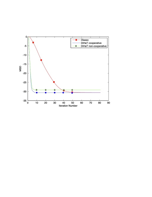
(a) MSD for the first experiment.

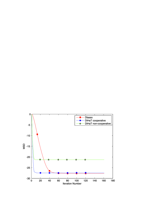
(b) MSD for the second experiment.

Figure 2: Average MSD Performance of the DiHat Algorithm

In the second experiment, the parameters remain the same as in the first one, but now a lower sparsity level, $\|\bm{h}_{*}\|_{\ell_{0}}=20$, is considered. As it can be seen from Fig. 2.b, the Dlasso outperforms significantly the non–cooperative counterpart of the DiHat. Nevertheless, the enhanced performance of the cooperative DiHaT, compared to the Dlasso, is retained. Intuitively, the previously mentioned behaviour is a consequence of the fact that a larger support set is more difficult to be identified, which can be seen from the performance degradation of the non–cooperative DiHaT. However, this problem can be overcome by identifying the support–set cooperatively, which enhances the performance of the DiHaT algorithm as illustrated in Fig. 2.b.

In the following experiments, we study the robustness of the DiHaT and the Dlasso algorithms, by their sensitivity to non “optimized” configurations. First of all, it is worth pointing out that a single user–defined parameter is employed in our proposed scheme (the sparsity level $s$), whereas in the Dlasso two user–defined parameters have to be tuned. The sensitivity of DiHaT on $s$ is examined. Moreover, we study how different choices of a parameter, which will be denoted by $c$ and is associated to the ADMM, affect the performance of the Dlasso. From Fig. 3, it can be readily seen that the DiHaT is rather insensitive if one sets the parameter $s$ to values larger than $\|\bm{h}_{*}\|_{\ell_{0}}$, which here equals to $10$. To be more specific, if $s=12$ then the algorithm converges slower, compared to the curve occurring by the optimized scenario, where $s=10$. Furthermore, if $s=16$ then we observe a slower convergence speed and a slightly higher error floor. Nevertheless, in both cases, the performance degradation and, consequently, the sensitiveness of the algorithm to the parameter $s$ is rather small. Fig. 5 illustrates the MSD curves of the Dlasso for the optimum choice of $c$, which equals to $0.3$, for $c=0.4$ and $c=0.5$. As it can be seen, the choice of this parameter affects significantly the convergence speed.

Figure 3: Sensitivity of the DiHaT to the $s$ parameter.

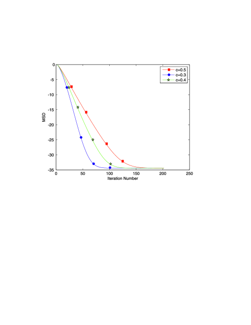
Figure 4: Sensitivity of the Dlasso to the $c$ parameter.

A drawback of the DiHaT compared to Dlasso is that the former requires a sufficient number of observations at each node, whereas the latter requires a certain number of data to be spread throughout the network. In particular, the DiHaT requires a RIP condition at node level, whereas the Dlasso does not make any assumptions regarding the number of measurements at each node. The goal of this experiment is twofold. The first goal is to shed light on the previously mentioned issue, by evaluating the performance of the algorithms in a scenario where each node has access to a small number of measurements. The second one is to validate the performance of a variation of the DiHaT algorithm, in which the nodes exchange and fuse estimate vectors solely. This is of significant interest in applications where exchanging measurement data is not feasible, due to energy/privacy constraints and in scenarios where the number of measurements varies from node to node and data fusion is not possible.

We consider the experimental set up of the first experiment where the number of measurements at each node equals $15$. As it can be seen from Fig 5, the non–cooperative greedy based algorithms fails to estimate the unknown vector accurately, since the error floor is high. On the contrary, the fully cooperative DiHaT as well as the DiHaT with estimate exchange exhibit an enhanced performance compared to that of the non–cooperative algorithm. Indeed, the full cooperative DiHaT converges relatively fast to a low error floor, whereas the DiHaT with estimate exchange converges to a significantly lower error floor compared to the non–cooperative algorithm, but larger compared to the DiHaT with data exchange. Finally, the Dlasso outperforms the greedy–based algorithms as it converges to the lowest error.

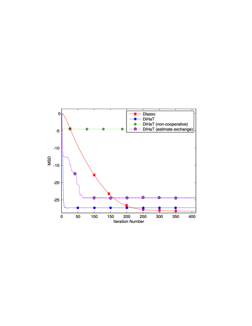
Figure 5: Performance evaluation in a scenario where the nodes have access to a small number of measurements.

VI-B Performance Evaluation of the GreeDi LMS

In this subsection, we present computer simulations of the adaptive variant of the proposed algorithm, and compare it against the sparsity promoting diffusion LMS–based scheme of [21] (SpaDLMS). The performance metric is the average Mean Square Deviation, which equals to $\mathrm{MSD}(n)=1/N\sum_{k=1}^{N}\|{\bm{h}}_{k}(n)-{\bm{h}}_{*}\|^{2}$ and the curves result from $100$ MC runs. At each MC run, a new sparsity pattern is generated and the non–zero elements of the parameter ${\bm{h}}_{*}$ for that run are draws from a multivariate Gaussian distribution ${\bm{h}}_{*|\mathcal{S}}\sim\mathcal{N}(0,\bm{I})$.

In the sixth experiment, we consider an ad–hoc network consisting of $N=10$ nodes. The unknown vector has dimension equal to $m=100$, with $10$ non–zero coefficients ($10\%$ sparsity ratio ($s/m$)). The input is drawn from a Gaussian distribution, with mean value equal to zero and variance equal to $1$, whereas the variance of the noise equals to $\sigma_{k}^{2}=0.01\eta_{k}\ \forall k\in{\mathcal{N}}$, where $\eta_{k}\in[0.5,1]$ is uniformly distributed. The combination coefficients are chosen with respect to the Metropolis rule. In this experiment, it is assumed that both algorithms are optimized in the sense that the regularization parameter used in [21] is chosen according to the optimum rule presented in this study, whereas in the proposed algorithm we assume that we know the number of non–zero coefficients. The regularization function, which enforces sparsity, is chosen similarly to the one proposed in [40]. Finally, the step–sizes are chosen so that the algorithms exhibit a similar convergence speed, and the forgetting factor $\zeta$ equals to $1$. From Fig. 6, it can be seen that the proposed algorithm outperforms SpaDLMS significantly, since it converges to a lower steady state error floor, at a similar convergence speed.

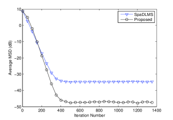
Figure 6: Average MSD for the sixth experiment. The stationary scenario.

In the seventh experiment, we examine the tracking behavior of the proposed scheme, i.e., the performance of the proposed algorithm in time–varying environments and the sensitivity in the case where our parameters are not optimized. In order to achieve these two goals, the following scenario is considered. We assume that at the first 1450 iterations the parameters are the same as in the first experiment, with the exception of the forgetting factor which now equals to $\zeta=0.99$. At the next time instant the channel undergoes a sudden change. Specifically, the number of non–zero coefficients equals to $15$. Notice that, the sparsity level for the GreeDi LMS is chosen equal to $15$, hence the parameter setting is no more “optimal”. From Fig. 7, it can be readily seen that the proposed algorithm enjoys a good tracking speed, since after the sudden change, it reaches at steady state, faster than the SpaDLMS.

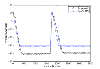
Figure 7: Average MSD for the seventh experiment. The time varying scenario.

Finally, in the eighth experiment, we study the performance of a modified version of the GreeDI LMS. To be more specific, we assume that the proxy is computed in a similar way as in [35] (see also Remark 3). In that case, the proxy computation involves operations between vectors and the complexity drops to $O(m)$. The parameters are the same as in the fifth experiment, and this modified algorithm is compared to the GreeDI LMS and the SpaDLMS. Furthermore, we include the GreeDI LMS, operating in a centralized mode, the performance of which serves as a benchmark. The step–sizes where chosen so that the decentralized algorithms exhibit a similar convergence speed. Finally, the step–size for the centralized algorithm equals to that of the decentralized one. Fig. 8 illustrates, that the GreeDI LMS outperforms both the “light” version of the GreeDI LMS and the SpaDLMS. Furthremore, the “light” GreeDI LMS converges to a lower error floor compared to the SpaDLMS. Finally, as it is expected, the centralized algorithm outperforms all the decentralized ones, since it exhibits a faster convergence speed.

Remark 4

It should be mentioned that the enhanced performance of the GreeDi LMS, compared to the SpaDLMS, comes at the expense of a higher complexity, since the complexity of the latter algorithm is of order $\mathcal{O}(m)$. Finally, the complexity of the “light” version of the GreeDI LMS is $\mathcal{O}(m)$ and each node transmits, at each time step, $2m$ coefficients, whereas the SpaDLMS requires the transmission of $m$ coefficients.

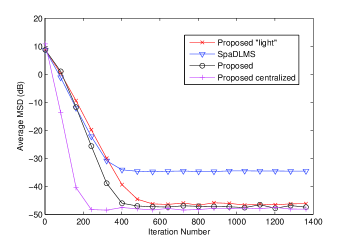
Figure 8: Average MSD for the eighth experiment. Performance evaluation of the “light” GreeDI LMS.

VII Conclusions

This work presented greedy methods for linear parameter estimation. Two operational modes were studied. Under the batch mode, where each node has access to a finite number of measurements, as well as on adaptive learning, where measurements arrive sequentially and the estimates are updated dynamically. The behavior of both schemes was analyzed theoretically and via simulations. The conditions, under which the batch algorithm converges are given whereas the adaptive algorithm is shown to converge, in the mean sense, and error bounds are derived. Future research will be focused on sparsity promoting algorithms for nonlinear distributed systems.

Appendix A Proof of Theorem 1

Let us define the networkwise vectors $\underline{\hat{{\bm{h}}}}_{n}=[{\hat{{\bm{h}}}}_{1,n}^{T},\ldots,{\hat{{\bm{h}}}}_{N,n}^{T}]^{T}\in{\mathbb{R}}^{Nm}$ and $\underline{\tilde{{\bm{h}}}}_{n}=[{\tilde{{\bm{h}}}}_{1,n}^{T},\ldots,{\tilde{{\bm{h}}}}_{N,n}^{T}]^{T}\in{\mathbb{R}}^{Nm}$. Using lemma 4.5 of [12], which provides a bound for the pruned estimate, we have that:

$$\|{{\underline{\bm{h}}}}_{n}-{\underline{\bm{h}}}_{*}\|_{\ell_{2}}\leq 2\|\underline{\tilde{{\bm{h}}}}_{n}-{\underline{\bm{h}}}_{*}\|_{\ell_{2}}.$$ (10)

Next, let us define the $Nm\times Nm$ consensus matrix, $\bm{P}$, which is defined as $\bm{P}=\bm{W}_{2}\otimes\bm{I}_{m}$, where the coefficients of the matrix $\bm{W}_{2}$ constitute the weights $b_{r,k}$. Recall that $\bm{P}\widetilde{{\underline{\bm{h}}}}=\widetilde{{\underline{\bm{h}}}},\ \forall\widetilde{{\underline{\bm{h}}}}\in\mathcal{O}$, where $\mathcal{O}\subset{\mathbb{R}}^{Nm}$ is the consensus subspace with definition $\mathcal{O}:=\{\widetilde{{\underline{\bm{h}}}}\in{\mathbb{R}}^{Nm}:\widetilde{{\underline{\bm{h}}}}=[\widetilde{{\bm{h}}}^{T},\ldots,\widetilde{{\bm{h}}}^{T}]^{T},\ \widetilde{{\bm{h}}}\in{\mathbb{R}}^{m}\}$. Moreover, recall that $\|\bm{P}\|=1$ (see [22]) and hence

$$\|\widetilde{{\underline{\bm{h}}}}_{n}-{\underline{\bm{h}}}_{*}\|_{\ell_{2}} =\|\bm{P}\underline{\hat{{\bm{h}}}}_{n}-{\underline{\bm{h}}}_{*}\|_{\ell_{2}}$$

$$=\|\bm{P}\underline{\hat{{\bm{h}}}}_{n}-\bm{P}{\underline{\bm{h}}}_{*}\|_{\ell_{2}}\leq\|\underline{\hat{{\bm{h}}}}_{n}-{\underline{\bm{h}}}_{*}\|_{\ell_{2}}.$$ (11)

Fix a node, say $k$. It holds that:

$$\|{\hat{{\bm{h}}}}_{k,n}-{\bm{h}}_{*}\|_{\ell_{2}}^{2}=\|({\hat{{\bm{h}}}}_{k,n}-{\bm{h}}_{*})_{\mathcal{S}_{k,n}}\|_{\ell_{2}}^{2}+\|({\hat{{\bm{h}}}}_{k,n}-{\bm{h}}_{*})_{{\mathcal{S}^{C}}_{k,n}}\|_{\ell_{2}}^{2}$$ (12)

Next, we will exploit results from [28, Theorem 3.5], where the distance between the estimate and the unknown vector restricted on the estimated support set or the complementary of this set, is given. So, following similar steps as in [28, Theorem 3.5], and taking into consideration Assumption 2.1, which states that for $n\geq n_{0}$ the noise term is negligible, the error term supported on the estimated support set satisfies

$$\|({\hat{{\bm{h}}}}_{k,n}-{\bm{h}}_{*})_{\mathcal{S}_{k,n}}\|_{\ell_{2}}\leq\delta_{2s}\|{\hat{{\bm{h}}}}_{k,n}-{\bm{h}}_{*}\|_{\ell_{2}}.$$ (13)

Moreover, according to [28, Theorem 3.5], the second term of the right hand side in (12) satisfies

$$\|({\hat{{\bm{h}}}}_{k,n}-{\bm{h}}_{*})_{{\mathcal{S}^{C}}_{k,n}}\|_{\ell_{2}}\leq\sqrt{2}\delta_{3s}\|{{{\bm{h}}}}_{k,n-1}-{\bm{h}}_{*}\|_{\ell_{2}}.$$ (14)

Combining (12)-(14) we arrive at the following inequality

$$\|{\hat{{\bm{h}}}}_{k,n}-{\bm{h}}_{*}\|_{\ell_{2}}\leq\sqrt{\frac{2\delta_{3s}^{2}}{1-\delta_{2s}^{2}}}\|{{{\bm{h}}}}_{k,n-1}-{\bm{h}}_{*}\|_{\ell_{2}}.$$ (15)

Taking into consideration (15), for the whole network we have

$$\|\underline{\hat{{\bm{h}}}}_{n}-\underline{{\bm{h}}}_{*}\|_{\ell_{2}}\leq\max_{k\in{\mathcal{N}}}\left\{\sqrt{\frac{2\delta_{3s}^{2}}{1-\delta_{2s}^{2}}}\right\}\|{\underline{{\bm{h}}}}_{n-1}-\underline{{\bm{h}}}_{*}\|_{\ell_{2}}.$$ (16)

Now, combining inequalities (10), (11), (16) it follows

$$\|\underline{{{\bm{h}}}}_{n}-\underline{{\bm{h}}}_{*}\|_{\ell_{2}}\leq\max_{k\in{\mathcal{N}}}\left\{\sqrt{\frac{8\delta_{3s}^{2(k,n)}}{1-\delta_{2s}^{2(k,n)}}}\right\}\|{\underline{{\bm{h}}}}_{n-1}-\underline{{\bm{h}}}_{*}\|_{\ell_{2}}.$$ (17)

Since by definition $\delta_{2s}^{(k,n)}\leq\delta_{3s}^{(k,n)}$, e.g., (see for instance [28]), and by assumption, $\delta_{3s}^{(k,n)}<\frac{1}{3},$ $\forall k\in{\mathcal{N}}$ it follows that $\max_{k\in{\mathcal{N}}}\left\{\sqrt{\frac{8\delta_{3s}^{2(k,n)}}{1-\delta_{2s}^{2(k,n)}}}\right\}<1$, and the proof is completed.

Appendix B Proof of Lemma 1

Under Assumption 3, we have that $\lim\limits_{n\rightarrow\infty}[\bm{R}_{k}(n)]_{ii}=\sigma_{k}^{2}$ (w.p.) $1$. So, recalling the definition of $\tilde{\nu}_{k}(n)$ we observe

$$\lim\limits_{n\rightarrow\infty}\tilde{\nu}_{k}(n) =\lim\limits_{n\rightarrow\infty}\sum_{r\in\mathcal{N}_{k}}b_{r,k}\frac{1}{m}\sum_{i=1}^{m}[\bm{R}_{r}(n)]_{ii}$$

$$=\sum_{r\in\mathcal{N}_{k}}b_{r,k}\frac{1}{m}\sum_{i=1}^{m}\lim\limits_{n\rightarrow\infty}[\bm{R}_{r}(n)]_{ii}=\sum_{r\in\mathcal{N}_{k}}b_{r,k}\sigma_{r}^{2}.$$ (18)

Now, since $\lim\limits_{n\rightarrow\infty}\overline{\bm{R}}_{k}(n)=\lim\limits_{n\rightarrow\infty}\sum_{r\in\mathcal{N}_{k}}b_{r,k}\bm{R}_{r}(n)=\sum_{r\in\mathcal{N}_{k}}b_{r,k}\sigma_{r}^{2}\bm{I}_{m}$ and from (18) it can be readily observed that

$$\lim\limits_{n\rightarrow\infty}\tilde{\mu}_{k}(n)\overline{\bm{R}}_{k}(n)=\bm{I}_{m}.$$ (19)

The vector used for the proxy computation, if $\|{\bm{h}}_{k}(n-1)\|_{\ell_{2}}\leq D$, can be rewritten as

$${\bm{h}}_{k}(n-1)+\tilde{\mu}_{k}(n)(\overline{\bm{p}}_{k}(n)-\overline{\bm{R}}_{k}(n){\bm{h}}_{k}(n-1))$$

$$=\left(\bm{I}_{m}-\tilde{\mu}_{k}(n)\overline{\bm{R}}_{k}(n)\right){\bm{h}}_{k}(n-1)+\tilde{\mu}_{k}(n)\overline{\bm{p}}_{k}(n)$$ (20)

and if $\|{\bm{h}}_{k}(n-1)\|_{\ell_{2}}>D$:

$$\frac{{\bm{h}}_{k}(n-1)}{\|{\bm{h}}_{k}(n-1)\|_{\ell_{2}}}+\tilde{\mu}_{k}(n)\left(\overline{\bm{p}}_{k}(n)-\overline{\bm{R}}_{k}(n)\frac{{\bm{h}}_{k}(n-1)}{\|{\bm{h}}_{k}(n-1)\|_{\ell_{2}}}\right)$$

$$=\left(\bm{I}_{m}-\tilde{\mu}_{k}(n)\overline{\bm{R}}_{k}(n)\right)\frac{{\bm{h}}_{k}(n-1)}{\|{\bm{h}}_{k}(n-1)\|_{\ell_{2}}}+\tilde{\mu}_{k}(n)\overline{\bm{p}}_{k}(n)$$ (21)

Let us first study the case where $\|{\bm{h}}_{k}(n-1)\|_{\ell_{2}}<D$. Taking into consideration (19) and (20) and the fact that $\|{\bm{h}}_{k}(n-1)\|_{\ell_{2}}<D$, we have that

$$\lim\limits_{n\rightarrow\infty}\left({\bm{h}}_{k}(n-1)+\tilde{\mu}_{k}(n)(\overline{\bm{p}}_{k}(n)-\overline{\bm{R}}_{k}(n){\bm{h}}_{k}(n-1))\right)$$ (22)

$$=\lim\limits_{n\rightarrow\infty}\tilde{\mu}_{k}(n)\overline{\bm{p}}_{k}(n)=\frac{1}{\overline{\sigma}_{k}^{2}}\overline{\bm{p}}_{k},$$ (23)

where $\overline{\sigma}_{k}^{2}:=\sum_{r\in{\mathcal{N}}_{k}}b_{r,k}{\sigma}_{l}^{2}$ and $\overline{\bm{p}}_{k}:=\sum_{r\in{\mathcal{N}}_{k}}b_{r,k}{\bm{p}}_{l}$. Obviously, if $\|{\bm{h}}_{k}(n-1)\|_{\ell_{2}}>D$ and if we combine (19) with (21), the same limit occurs. From the Wiener–Hopf equation, e.g., [39], it holds that

$$\frac{1}{\overline{\sigma}_{k}^{2}}\overline{\bm{p}}_{k}=\frac{1}{\overline{\sigma}_{k}^{2}}\sum_{r\in\mathcal{N}_{k}}{b_{r,k}}\bm{R}_{r}\bm{h}_{*}.$$ (24)

Nevertheless, from the diagonality of the matrices $\bm{R}_{k},\ \forall k\in{\mathcal{N}}$ (Assumption 3.2), it can be readily obtained from (24) that

$$\mathrm{supp}\left(\frac{1}{\overline{\sigma}_{k}^{2}}\overline{\bm{p}}_{k}\right)=\mathcal{S}$$ (25)

Equations (23) and (25) complete our proof, since the proxy converges to a vector, which has the same support set as ${\bm{h}}_{*}$ and obviously, after a finite number of iterations the $s$–largest in magnitude coefficients of these two vectors will coincide. Intuitively, the fact that the proxy converges to a vector, with the same support set as ${\bm{h}}_{*}$ implies that these two vectors will be arbitrarily close $n\geq n_{0}$, for a sufficiently large $n_{0}$. If the $s$ largest in amplitude coefficients of the proxy, do not coincide with the positions of the true support set, then a coefficient of the proxy, say in the position $i_{0}\notin\mathcal{S}$ will be larger in amplitude than a coefficient $i_{0}^{\prime}\in\mathcal{S}$. This contradicts the fact that the previously mentioned vectors will be arbitrarily close, since their distance will be at least larger than the amplitude of the coefficient $i_{0}$ of the proxy.

Appendix C Proof of Theorem 3

Notice that from the previous Lemma, $\forall n\geq n_{0},\ \forall k\in{\mathcal{N}}$ the algorithmic scheme drops to the Adapt–Combine LMS presented in [30]. Now, let us define the networkwise error vector $\tilde{\underline{{\bm{h}}}}(n)=[{\bm{h}}_{1}^{T}(n)-{\bm{h}}_{*}^{T},\ldots,\bm{h}_{N}^{T}(n)-{\bm{h}}_{*}^{T}]^{T}\in{\mathbb{R}}^{Nm}$. Using similar arguments as in [30] we have that $\forall n\geq n_{0}$ the error vector for the whole network can be written as follows

$$\tilde{\underline{\bm{h}}}(n)=\bm{P}\left(\tilde{\underline{{\bm{h}}}}(n-1)-\mathcal{M}[\bm{D}(n)\underline{{\bm{h}}}(n-1)+\bm{G}(n)]\right),$$ (26)

where $\mathcal{M}=\mathrm{diag}\{\mu_{1}\bm{I}_{m},\ldots,\mu_{N}\bm{I}_{m}\}$, $\bm{D}(n)=\mathrm{diag}\{\bm{a}_{1}(n)\bm{a}_{1}^{T}(n),\ldots\,\bm{a}_{N}(n)\bm{a}_{N}^{T}(n)\}$,$\bm{G}(n)=[\bm{a}_{1}^{T}(n){v}_{1}(n),\ldots\,\bm{a}^{T}_{N}(n){v}_{N}(n)]^{T}$ and $\bm{P}$ is the $Nm\times Nm$ consensus matrix, which contains the combination coefficients $c_{r,k},\ \forall k\in{\mathcal{N}},\forall r\in{\mathcal{N}}_{k}$, e.g., [22].

Taking expectation in (26) and taking into consideration the assumptions we have that

$$E[\tilde{\underline{\bm{h}}}(n)]=\bm{P}\left(\bm{I}_{Nm}-\mathcal{M}\mathcal{D}\right)E[\tilde{\underline{\bm{h}}}(n-1)],\ \forall n\geq n_{0}$$ (27)

where $\bm{I}_{Nm}$ is the identity matrix of dimension $Nm\times Nm$ and $\mathcal{D}:=\mathrm{diag}\{\bm{R}_{1},\ldots,\bm{R}_{N}\}$. According to [30, Lemma 1] the matrix $\bm{P}\left(\bm{I}_{Nm}-\mathcal{M}\mathcal{D}\right)$ is a stable matrix, i.e., all its eigenvalues lie inside the unit circle. Iterating (27) we obtain

$$\|E[\tilde{\underline{\bm{h}}}(n)]\|_{\ell_{2}} \leq\lambda_{\max}\left(\bm{P}\left(\bm{I}_{Nm}-\mathcal{M}\mathcal{D}\right)\right)\|E[\tilde{\underline{\bm{h}}}(n-1)]\|_{\ell_{2}}$$

$$\leq\lambda_{\max}\left(\bm{P}\left(\bm{I}_{Nm}-\mathcal{M}\mathcal{D}\right)\right)^{n-n_{0}}\|E[\tilde{\underline{\bm{h}}}(n_{0})]\|_{\ell_{2}}\rightarrow 0,\ n\rightarrow\infty.$$

The last relation completes our proof.

Appendix D Steady State Analysis

Fix an arbitrary node $k\in{\mathcal{N}}$, by employing the triangle inequality, it holds for the local error that

$$\|\bm{\psi}_{k}(n)-{\bm{h}}_{*}\|_{\ell_{2}} \leq\|\left(\bm{\psi}_{k}(n)-{\bm{h}}_{*}\right)_{|\widehat{\mathcal{S}}_{k,n}}\|$$

$$+\|\left(\bm{\psi}_{k}(n)-{\bm{h}}_{*}\right)_{|\widehat{\mathcal{S}}_{k,n}^{c}}\|$$ (28)

Let us analyse each individual term of the right hand side of (28). We obtain the following cases:

• $\|{\bm{h}}_{k}(n-1)\|\leq D$:

  Following identical steps as in [28, Thm. 3.8] it holds that

  $$\|\left(\bm{\psi}_{k}(n)-{\bm{h}}_{*}\right)_{|\widehat{\mathcal{S}}_{k,n}^{c}}\|_{\ell_{2}} \leq\sqrt{2}\Big{[}\delta_{3s,k}(\lambda,n)\|\bm{h}_{k}(n-1)$$

  $$-{\bm{h}}_{*}\|_{\ell_{2}}+\|\overline{\bm{\eta}}_{k}(n)\|_{\ell_{2}}\Big{]}$$ (29)

• $\|{\bm{h}}_{k}(n-1)\|>D$.

  Again, following similar steps as in [28, Thm. 3.8] we obtain that:

  $$\|\left(\bm{\psi}_{k}(n)-{\bm{h}}_{*}\right)_{|\widehat{\mathcal{S}}_{k,n}^{c}}\|_{\ell_{2}}\leq$$

  $$\sqrt{2}\left[\delta_{3s,k}(\lambda,n)\left\|\frac{\bm{h}_{k}(n-1)}{\|\bm{h}_{k}(n-1)\|}-{\bm{h}}_{*}\right\|_{\ell_{2}}+\|\overline{\bm{\eta}}_{k}(n)\|_{\ell_{2}}\right].$$ (30)

  Recall that $\|{\bm{h}}_{k}(n-1)\|>D\linebreak\geq 2\|{\bm{h}}_{*}\|_{\ell_{2}}+1$. Exploiting the triangle inequality, it holds that

  $$\left\|\frac{\bm{h}_{k}(n-1)}{\|\bm{h}_{k}(n-1)\|}-{\bm{h}}_{*}\right\|_{\ell_{2}}\leq 1+\|{\bm{h}}_{*}\|_{\ell_{2}},$$

  and

  $$\|{\bm{h}_{k}(n-1)} -{\bm{h}}_{*}\|_{\ell_{2}}\geq\|{\bm{h}_{k}(n-1)}\|_{\ell_{2}}$$

  $$-\|{\bm{h}}_{*}\|_{\ell_{2}}\geq\|{\bm{h}}_{*}\|_{\ell_{2}}+1.$$

  The previous inequalities imply that

  $$\left\|\frac{\bm{h}_{k}(n-1)}{\|\bm{h}_{k}(n-1)\|}-{\bm{h}}_{*}\right\|_{\ell_{2}}\leq\|{\bm{h}_{k}(n-1)}-{\bm{h}}_{*}\|_{\ell_{2}},$$

  and combining this with (30), we obtain that

  $$\|\left(\bm{\psi}_{k}(n)-{\bm{h}}_{*}\right)_{|\widehat{\mathcal{S}}_{k,n}^{c}}\|_{\ell_{2}}$$

  $$\leq\sqrt{2}\Big{[}\delta_{3s,k}(\lambda,n)\|\bm{h}_{k}(n-1)-{\bm{h}}_{*}\|_{\ell_{2}}$$

  $$+\sqrt{1+\delta_{2s,k}(\lambda,n)}\|\overline{\bm{\eta}}_{k}(n)\|_{\ell_{2}}\Big{]}.$$

Hence, the inequality in (30) holds for both the proxy selection vectors.

Remark 5

The proxy noise disturbance $\overline{\bm{\eta}}_{k}(n)$ involves a double averaging (across neighbour and exponential average on each time instant) of two independent variables.

Next we analyse the first term of the right hand side of Eq. (28). At each iteration, the Least–Mean-Square recursive relation (restricted at the local estimated support set $\widehat{\mathcal{S}}_{k,n}$)

$$\bm{\psi}_{k|\widehat{\mathcal{S}}_{k,n}}(n) =\bm{h}_{k|\widehat{\mathcal{S}}_{k,n}}(n-1)$$

$$+\mu_{k}\bm{a}_{k|\widehat{\mathcal{S}}_{k,n}}(n)\left[y_{k}(n)-\bm{a}^{T}_{k|\widehat{\mathcal{S}}_{k,n}}(n)\bm{h}_{k|\widehat{\mathcal{S}}_{k,n}}(n-1)\right]$$ (31)

updates the coefficient vector. Next we rewrite the restricted LMS iteration in term of the error vector $(\bm{\psi}_{k}(n)-{\bm{h}}_{*})_{k|\widehat{\mathcal{S}}_{k,n}}$ to obtain

$$(\bm{\psi}_{k}(n)-{\bm{h}}_{*})_{k|\widehat{\mathcal{S}}_{k,n}}=\left(\bm{h}_{k}(n-1)-{\bm{h}}_{*}\right)_{|\widehat{\mathcal{S}}_{k,n}}$$

$$+\mu_{k}\bm{a}_{k|\widehat{\mathcal{S}}_{k,n}}(n)\left[y_{k}(n)-\bm{a}^{T}_{k|\widehat{\mathcal{S}}_{k,n}}(n)\bm{h}_{k|\widehat{\mathcal{S}}_{k,n}}(n-1)\right]$$

$$=\left(\bm{h}_{k}(n-1)-{\bm{h}}_{*}\right)_{|\widehat{\mathcal{S}}_{k,n}}+\mu_{k}\bm{a}_{k|\widehat{\mathcal{S}}_{k,n}}(n)\left[y_{k}(n)-\bm{a}^{T}_{k}(n){\bm{h}}_{*}\right]$$

$$+\mu_{k}\bm{a}_{k|\widehat{\mathcal{S}}_{k,n}}(n)\left[\bm{a}^{T}_{k}(n){\bm{h}}_{*}-\bm{a}^{T}_{k|\widehat{\mathcal{S}}_{k,n}}(n)\bm{h}_{k|\widehat{\mathcal{S}}_{k,n}}(n-1)\right]$$

$$=\left(\bm{I}_{m}-\mu_{k}\bm{a}_{k|\widehat{\mathcal{S}}_{k,n}}(n)\bm{a}^{T}_{k|\widehat{\mathcal{S}}_{k,n}}(n)\right)\left(\bm{h}_{k}(n-1)-{\bm{h}}_{*}\right)_{|\widehat{\mathcal{S}}_{k,n}}$$

$$+\mu_{k}\bm{a}_{k|\widehat{\mathcal{S}}_{k,n}}(n)e_{0,k}(n)+\mu_{k}\bm{a}_{k|\widehat{\mathcal{S}}_{k,n}}(n)\bm{a}^{T}_{k|{\mathcal{S}}\setminus\widehat{\mathcal{S}}_{k,n}}(n){\bm{h}}_{*|{\mathcal{S}}\setminus\widehat{\mathcal{S}}_{k,n}}$$ (32)

where $e_{0,k}(n):=y_{k}(n)-\bm{a}^{T}_{k}(n){\bm{h}}_{*}$ in the adaptive filtering literature is referred to as the estimation error of the optimum Wiener solution $\bm{h}_{*}$ to the normal equations

$$\bm{R}_{k}\bm{h}=\bm{p}_{k}$$ (33)

with $\bm{R}_{k}:=\mathbb{E}[\bm{a}_{k}(n)\bm{a}_{k}^{T}(n)]$ and $\bm{p}_{k}:=\mathbb{E}[y_{k}(n)\bm{a}_{k}(n)]$. The recursion of Eq. (32) can be written in terms of the weight–error–vectors

$$\epsilon_{k}^{(1)}(n):=\|\bm{\psi}_{k}(n)-{\bm{h}}_{*}\|_{\ell_{2}}$$ (34)

$$\epsilon_{k}^{(2)}(n):=\|\bm{h}_{k}(n)-{\bm{h}}_{*}\|_{\ell_{2}}$$ (35)

Additionally we invoke the Direct–Averaging method [39], provided that the step size $\mu_{k}$ is small, where the regression correlation terms $\bm{a}_{k}(n)\bm{a}_{k}^{T}(n)$ in Eq. (32) are approximated with its average (the autocorrelation matrix $\bm{R}_{k}$). Hence, Eq. (32) becomes

$$\epsilon_{k|\widehat{\mathcal{S}}_{k,n}}^{(1)}(n) \leq(1-\mu_{k}\lambda_{min})\epsilon_{k|\widehat{\mathcal{S}}_{k,n}}^{(2)}(n-1)+\mu_{k}\|\bm{a}_{k|\widehat{\mathcal{S}}_{k,n}}^{T}\|_{\ell_{2}}(n)|e_{o,k}(n)|$$

$$+\mu_{k}\|\bm{a}_{k|\widehat{\mathcal{S}}_{k,n}}(n)\bm{a}^{T}_{k|{\mathcal{S}}\setminus\widehat{\mathcal{S}}_{k,n}}(n)\|_{\ell_{2}}\|{\bm{h}}_{*|{\mathcal{S}}\setminus\widehat{\mathcal{S}}_{k,n}}\|_{\ell_{2}}$$ (36)

and $\lambda_{min}$ is the minimum eigenvalue of $\bm{R}_{k}$ [39, p. 168], assuming that that it is non singular (i.e. $\lambda_{min}>0$). Note that unlike the batch variants of the proposed algorithm (into their centralized form, i.e. [28, 41]), the proposed algorithm is not applied to a fixed block of measurements. Therefore, the analysis of the proposed algorithm needs to take into account time dependencies at the support of $\bm{h}_{k}(n)$. The changes in the support of the local estimate across different $n$ are considered via the following expression:

$$\epsilon_{k|\widehat{\mathcal{S}}_{k,n}}^{(1)}(n)$$

$$\leq(1-\mu_{k}\lambda_{min})\left\|\left(\bm{h}_{k}(n-1)-{\bm{h}}_{*}\right)_{|\widehat{\mathcal{S}}_{k,n}}+\left(\bm{h}_{k}(n-1)-{\bm{h}}_{*}\right)_{|\widehat{\mathcal{S}}_{k,n-1}}\right.$$

$$\left.+\left({\bm{h}}_{*}-\bm{h}_{k}(n-1)\right)_{|\widehat{\mathcal{S}}_{k,n-1}}\right\|_{\ell_{2}}+\mu_{k}\|\bm{a}_{k|\widehat{\mathcal{S}}_{k,n}}^{T}(n)\|_{\ell_{2}}|e_{o,k}(n)|$$

$$+\mu_{k}\|\bm{a}_{k|\widehat{\mathcal{S}}_{k,n}}(n)\bm{a}^{T}_{k|{\mathcal{S}}\setminus\widehat{\mathcal{S}}_{k,n}}(n)\|_{\ell_{2}}\|{\bm{h}}_{*|{\mathcal{S}}\setminus\widehat{\mathcal{S}}_{k,n}}\|_{\ell_{2}}$$ (37)

$$\epsilon_{k|\widehat{\mathcal{S}}_{k,n}}^{(1)}(n) \leq(1-\mu_{k}\lambda_{min})\left\{\epsilon_{k|\widehat{\mathcal{S}}_{k,n}}^{(2)}(n-1)+2\epsilon_{k|\widehat{\mathcal{S}}_{k,n-1}}^{(2)}(n-1)\right\}$$

$$+\mu_{k}\|\bm{a}_{k|\widehat{\mathcal{S}}_{k,n}}^{T}(n)\|_{\ell_{2}}|e_{o,k}(n)|$$

$$+\mu_{k}\|\bm{a}_{k|\widehat{\mathcal{S}}_{k,n}}(n)\bm{a}^{T}_{k|{\mathcal{S}}\setminus\widehat{\mathcal{S}}_{k,n}}(n)\|_{\ell_{2}}\|{\bm{h}}_{*|{\mathcal{S}}\setminus\widehat{\mathcal{S}}_{k,n}}\|_{\ell_{2}}$$ (38)

Now we want to express the fourth term of Eq. (38) in terms of $\epsilon_{k}^{(2)}(n-1)$. From Theorem 3.8 of [28] and the direct–averaging method, one can write

$$\|\bm{a}_{k|\widehat{\mathcal{S}}_{k,n}}(n)\bm{a}^{T}_{k|{\mathcal{S}}\setminus\widehat{\mathcal{S}}_{k,n}}(n)\|_{\ell_{2}}\|{\bm{h}}_{*|{\mathcal{S}}\setminus\widehat{\mathcal{S}}_{k,n}}\|$$

$$\leq\|\bm{R}_{k}\|_{\ell_{2}}\|\left(\bm{\psi}_{k}(n)-{\bm{h}}_{*}\right)_{\widehat{\mathcal{S}}^{c}_{k,n}}\|_{\ell_{2}}=\lambda_{\max}\epsilon_{k|\widehat{\mathcal{S}}^{c}_{k,n}}^{(1)}(n)$$

$$\leq \sqrt{2}\lambda_{\max}\left[\delta_{3s,k}(\lambda,n)\epsilon_{k}^{(2)}(n-1)+\sqrt{1+\delta_{2s,k}(\lambda,n)}\|\overline{\bm{\eta}}_{k}(n)\|_{\ell_{2}}\right]$$ (39)

By combining Eqs. (38), (39), (29) in Eq. (28) we obtain the following recurrence

$$\epsilon_{k}^{(1)}(n) \leq(1-\mu_{k}\lambda_{min})\left\{\epsilon_{k|\widehat{\mathcal{S}}_{k,n}}^{(2)}(n-1)+2\epsilon_{k|\widehat{\mathcal{S}}_{k,n-1}}^{(2)}(n-1)\right\}$$

$$+\sqrt{2}\delta_{3s,k}(\lambda,n)\left(1+\mu_{k}\lambda_{\max}\right)\epsilon_{k}^{(2)}(n-1)$$

$$+\sqrt{2}\sqrt{1+\delta_{2s,k}(\lambda,n)}\left(1+\mu_{k}\lambda_{\max}\right)\|\overline{\bm{\eta}}_{k}(n)\|_{\ell_{2}}$$

$$+\mu_{k}\|\bm{a}_{k|\widehat{\mathcal{S}}_{k,n}}^{T}(n)\|_{\ell_{2}}|e_{o,k}(n)|$$ (40)

Note that, the following two inequalities hold: $\epsilon_{k|\widehat{\mathcal{S}}_{k,n-1}}^{(2)}(n-1)\leq\epsilon_{k}^{(2)}(n-1)$ and $\epsilon_{k|\widehat{\mathcal{S}}_{k,n}}^{(2)}(n-1)\leq\epsilon_{k}^{(2)}(n-1)$ so that

$$\epsilon_{k}^{(1)}(n) \leq\Big{[}3(1-\mu_{k}\lambda_{min})$$

$$+\sqrt{2}\delta_{3s,k}(\lambda,n)\left(1+\mu_{k}\lambda_{\max}\right)\Big{]}\epsilon_{k}^{(2)}(n-1)$$

$$+\sqrt{2}\sqrt{1+\delta_{2s,k}(\lambda,n)}\left(1+\mu_{k}\lambda_{\max}\right)\|\overline{\bm{\eta}}_{k}(n)\|_{\ell_{2}}$$

$$+\mu_{k}\|\bm{a}_{k|\widehat{\mathcal{S}}_{k,n}}^{T}(n)\|_{\ell_{2}}|e_{o,k}(n)|$$ (41)

Finally, for the whole network we have

$$\underline{\epsilon}(n)\leq 2N\max_{k\in\mathcal{N}}\Big{\{}3(1-\mu_{k}\lambda_{min})+\sqrt{2}\delta_{3s,k}(\lambda,n)$$

$$\left(1+\mu_{k}\lambda_{\max}\right)\Big{\}}\sum_{k=1}^{N}\epsilon_{k}^{(2)}(n-1)$$

$$+2N\max_{k\in\mathcal{N}}\left\{\sqrt{2}\sqrt{1+\delta_{2s,k}(\lambda,n)}\left(1+\mu_{k}\lambda_{\max}\right)\right\}\sum_{k=1}^{N}\|\overline{\bm{\eta}}_{k}(n)\|_{\ell_{2}}$$

$$+2N\max_{k\in\mathcal{N}}\left\{\mu_{k}\|\bm{a}_{k|\widehat{\mathcal{S}}_{k,n}}^{T}(n)\|_{\ell_{2}}\right\}\sum_{k=1}^{N}|e_{o,k}(n)|$$ (42)

We arrived at Eq. (42) by recalling Remark 3. The second term on the right hand side of the Eq. (42) reminds us the steady–state error of the HTP algorithm [28] (mainly because we are using an exponentially weighted average proxy variant of [28]), whereas the first and second term are introduced due to the usage of the diffusion LMS algorithm instead of the LS estimator.

References

- [1] A. M. Bruckstein, D. L. Donoho, and M. Elad, “From sparse solutions of systems of equations to sparse modeling of signals and images,” SIAM review, vol. 51, no. 1, pp. 34–81, 2009.
- [2] S. Theodoridis, Y. Kopsinis, and K. Slavakis, “Sparsity–aware learning and compressed sensing: An overview,” arXiv preprint arXiv:1211.5231, 2012.
- [3] M. Elad, Sparse and Redundant Representations, Springer, 2010.
- [4] Behtash Babadi, Nicholas Kalouptsidis, and Vahid Tarokh, “Sparls: The sparse RLS algorithm,” IEEE Transactions on Signal Processing, vol. 58, no. 8, pp. 4013–4025, 2010.
- [5] S.J. Godsill A.Y. Carmi, L. Mihaylova, Ed., Compressed Sensing & Sparse Filtering, Springer, 2014.
- [6] S. Theodoridis, Machine Learning: A Signal and Information Processing and Analysis Perspective, Academic Press, 2015.
- [7] Jimmy Lin, “Mapreduce is good enough? If all you have is a hammer, throw away everything that’s not a nail!,” Big Data, vol. 1, no. 1, pp. 28–37, 2013.
- [8] S. Boyd, N. Parikh, E. Chu, B. Peleato, and J. Eckstein, “Distributed optimization and statistical learning via the alternating direction method of multipliers,” Foundations and Trends in Machine Learning, vol. 3, no. 1, pp. 1–122, 2011.
- [9] J.A. Tropp and S.J. Wright, “Computational methods for sparse solution of linear inverse problems,” Proceedings of the IEEE, vol. 98, no. 6, pp. 948 –958, 2010.
- [10] Joel A Tropp, “Greed is good: Algorithmic results for sparse approximation,” IEEE Transactions on Information Theory, vol. 50, no. 10, pp. 2231–2242, 2004.
- [11] David L Donoho, Yaakov Tsaig, Iddo Drori, and J-L Starck, “Sparse solution of underdetermined systems of linear equations by stagewise orthogonal matching pursuit,” IEEE Transactions on Information Theory, vol. 58, no. 2, pp. 1094–1121, 2012.
- [12] D. Needell and J.A. Tropp, “Cosamp: Iterative signal recovery from incomplete and inaccurate samples,” Applied and Computational Harmonic Analysis, vol. 26, no. 3, pp. 301 – 321, 2009.
- [13] Wei Dai and Olgica Milenkovic, “Subspace pursuit for compressive sensing signal reconstruction,” IEEE Trans. on Information Theory, vol. 55, no. 5, pp. 2230–2249, 2009.
- [14] D. Needell and R. Vershynin, “Uniform uncertainty principle and signal recovery via regularized orthogonal matching pursuit,” Found. Comput. Math, vol. 9, no. 3, pp. 317–334, 2009.
- [15] Honglin Huang and A. Makur, “Backtracking-based matching pursuit method for sparse signal reconstruction,” IEEE Signal Processing Letters, vol. 18, no. 7, pp. 391–394, 2011.
- [16] T. Peleg, Y.C. Eldar, and M. Elad, “Exploiting statistical dependencies in sparse representations for signal recovery,” IEEE Transactions on Signal Processing, vol. 60, no. 5, pp. 2286–2303, 2012.
- [17] V. Temlyakov, Greedy Approximation, Cambridge University Press, 2011.
- [18] G. Mateos, J.A. Bazerque, and G.B. Giannakis, “Distributed sparse linear regression,” IEEE Trans. Signal Process., vol. 58, no. 10, pp. 5262–5276, 2010.
- [19] João FC Mota, João MF Xavier, Pedro MQ Aguiar, and Markus Püschel, “Distributed basis pursuit,” IEEE Transactions on Signal Processing, vol. 60, no. 4, pp. 1942–1956, 2012.
- [20] Stacy Patterson, Yonina C Eldar, and Idit Keidar, “Distributed sparse signal recovery for sensor networks,” in IEEE International Conference on Acoustics, Speech and Signal Processing (ICASSP). IEEE, 2013, pp. 4494–4498.
- [21] P. Di Lorenzo and A.H. Sayed, “Sparse distributed learning based on diffusion adaptation,” IEEE Transactions on Signal Processing, vol. 61, no. 6, pp. 1419–1433, 2013.
- [22] S. Chouvardas, K. Slavakis, Y. Kopsinis, and S. Theodoridis, “A sparsity promoting adaptive algorithm for distributed learning,” IEEE Trans. Signal Process., vol. 60, no. 10, pp. 5412 –5425, 2012.
- [23] Zhaoting Liu, Ying Liu, and Chunguang Li, “Distributed sparse recursive least-squares over networks,” IEEE Transactions on Signal Processing, vol. 62, pp. 1386–1395, 2014.
- [24] Chris Clifton, Murat Kantarcioglu, Jaideep Vaidya, Xiaodong Lin, and Michael Y Zhu, “Tools for privacy preserving distributed data mining,” ACM SIGKDD Explorations Newsletter, vol. 4, no. 2, pp. 28–34, 2002.
- [25] Ali H Sayed, “Diffusion adaptation over networks,” arXiv preprint arXiv:1205.4220, 2012.
- [26] Dimitri P Bertsekas and John N Tsitsiklis, Parallel and distributed computation: Numerical Methods, Athena-Scientific, second edition, 1999.
- [27] Pedro A Forero, Alfonso Cano, and Georgios B Giannakis, “Consensus-based distributed support vector machines,” The Journal of Machine Learning Research, vol. 99, pp. 1663–1707, 2010.
- [28] S. Foucart, “Hard thresholding pursuit: An algorithm for compressive sensing,” SIAM Journal on Numerical Analysis, vol. 49, no. 6, pp. 2543–2563, 2011.
- [29] C.G. Lopes and A.H. Sayed, “Diffusion least-mean squares over adaptive networks: Formulation and performance analysis,” IEEE Trans. Signal Process., vol. 56, no. 7, pp. 3122–3136, 2008.
- [30] F.S. Cattivelli and A.H. Sayed, “Diffusion LMS strategies for distributed estimation,” IEEE Trans. Signal Process., vol. 58, no. 3, pp. 1035 –1048, 2010.
- [31] S. Chouvardas, K. Slavakis, and S. Theodoridis, “Adaptive robust distributed learning in diffusion sensor networks,” IEEE Trans. Signal Process.g, vol. 59, no. 10, pp. 4692–4707, 2011.
- [32] I.D. Schizas, G. Mateos, and G.B. Giannakis, “Distributed LMS for consensus-based in-network adaptive processing,” IEEE Trans. Signal Process., vol. 57, no. 6, pp. 2365 –2382, 2009.
- [33] S.Y. Tu and A.H. Sayed, “Diffusion networks outperform consensus networks,” in IEEE Workshop of SSP, 2012, pp. 313–316.
- [34] A.H. Sayed, Adaptive Filters, John Wiley and Sons, 2008.
- [35] G. Mileounis, B. Babadi, N. Kalouptsidis, and V. Tarokh, “An adaptive greedy algorithm with application to nonlinear communications,” IEEE Trans. Signal Process., vol. 58, no. 6, pp. 2998 –3007, 2010.
- [36] L. Xiao and S. Boyd, “Fast linear iterations for distributed averaging,” Systems & Control Letters, vol. 53, no. 1, pp. 65–78, 2004.
- [37] Renato LG Cavalcante, Isao Yamada, and Bernard Mulgrew, “An adaptive projected subgradient approach to learning in diffusion networks,” Signal Processing, IEEE Transactions on, vol. 57, no. 7, pp. 2762–2774, 2009.
- [38] Athanasios Papoulis and S Unnikrishna Pillai, Probability, random variables, and stochastic processes, Tata McGraw-Hill Education, 2002.
- [39] S. Haykin, Adaptive Filter Theory, Prentice Hall, 1996.
- [40] P. Di Lorenzo, S. Barbarossa, and A.H. Sayed, “Distributed spectrum estimation for small cell networks based on sparse diffusion adaptation,” IEEE Signal Processing Letters, vol. 20, no. 12, pp. 1261–1265, Dec 2013.
- [41] Thomas Blumensath and Mike E. Davies, “Iterative hard thresholding for compressed sensing,” Applied and Computational Harmonic Analysis, vol. 27, no. 3, pp. 265 – 274, 2009.