Experimental on-demand recovery of entanglement by local operations within non-Markovian dynamics
Abstract
In many applications entanglement must be distributed through noisy communication channels that unavoidably degrade it. Entanglement cannot be generated by local operations and classical communication (LOCC), implying that once it has been distributed it is not possible to recreate it by LOCC. Recovery of entanglement by purely local control is however not forbidden in the presence of non-Markovian dynamics, and here we demonstrate in two all-optical experiments that such entanglement restoration can even be achieved on-demand. First, we implement an open-loop control scheme based on a purely local operation, without acquiring any information on the environment; then, we use a closed-loop scheme in which the environment is measured, the outcome controling the local operations on the system. The restored entanglement is a manifestation of "hidden" quantum correlations resumed by the local control. Relying on local control, both schemes improve the efficiency of entanglement sharing in distributed quantum networks.
Quantum mechanics promises breakthroughs in computing and information fields, some of which are already available lunghi2013 ; ekert2014 . Similarly to networking in classical information and computation, the advent of quantum networks envisages further advancements in information science kimble2008 ; sciarrino2012 ; perseguers2013 . Tasks such as measurements, computing and memorization may be performed by subsystems implemented on different platforms hybrid , networking also providing the large amount of resources required to fault tolerant computation schemes steane1998 ; preskill1998 . Recent experimental up-scaling of quantum processors made it clear that for hardware-intrinsic noise sources the low-decoherence DiVincenzo criterion divincenzo2000 could be met by subsystems of limited size ladd2010 in distributed architectures. This is a new, and uniquely "quantum" feature of networking.
The roadmap towards distributed networks critically relies on the possibility that pairs (or clusters) of nodes share entanglement PlenioReview ; HorodeckiReview . This is the fundamental resource allowing remote quantum teleportation bennett1993 ; zeilinger1997 ; boschi1998 ; ursin2007 of an unknown quantum state or secure keys distribution for cryptographic purposes gisin2002 . In particular for the scope of our work it is important to note that entanglement could enable universal quantum computation in networks of noninteracting nodes, provided single qubit local operations are possible gottesman1999 . Sharing entanglement can reduce the communication complexity, that is the minimal information exchange required to solve a given problem distributed among separated parts bruckner2004 . Very recently, it has been proposed that entanglement may improve accuracy and precision in applications related to global positioning and timing by networking geographically remote atomic clocks komer2014 .
In order to use entanglement as a non-local resource PlenioReview ; HorodeckiReview , it must be generated somewhere and then distributed amongst different parties. However noise unavoidably affects distribution and storage of entanglement, determining its degradation. It is well known that different parties cannot create any further entanglement, if they are only allowed to operate locally, i.e. on their own subsystem, exchanging at most classical information bennett1996 .
Our scope is distributed networks of spatially separated quantum nodes, each subject to a local environment. They model the structure of physically relevant distributed architectures. Remarkably, when environments induce a system dynamics which can be physically unraveled into an ensemble of entangled pure state evolutions, it may happen that quantum correlations of initially entangled states are not destroyed. Indeed even if entanglement appears degraded when measured on the averaged state, it is not lost but rather hidden in the lack of classical knowledge about the elements of the ensemble darrigo2014Annals . In this case, leveraging the existence of such classical information, the initially shared entanglement can be restored at an arbitrary time without resorting to non-local operations.
An operational scenario emerges in which local controls can be used for on-demand restoration of entanglement in distributed architectures. Here we demonstrate this concept by two all-optical experiments. We consider two entangled photons subject to local environments as an instance of distributed entanglement. In the first experiment a local environment produces low-frequency noise PaladinoReview2013 , and it is shown how by local open loop control vandersypen2005 the initial entanglement is recovered, even if in the absence of control it would be degraded to very low values. In the second experiment, decoherence is due to the coupling between a subsystem (photon) and a quantum environment, whose degrees of freedom are experimentally accessible. A measurement on this environment and a subsequent conditional local operation on the system implement a local closed-loop control wiseman2010book , succeeding in restoring the initial entanglement. The relevance of these setups to different physical systems is discussed at the end of this work.
The non-Markovian nature of the dynamics cohen-Tannoudji ; rivas2014 is a key ingredient for the entanglement recovery in our experiments. Certain physical aspects are common to other phenomena involving non-Markovianity, such as spontaneous entanglement revivals during the system dynamics bellomo2007PRL ; liu_natphys_2011 ; chiu2012 ; lofranco2012PRA ; xu_natcomm_2013 , or entanglement preservation by dynamical decoupling wang2011 ; roy_pra_2011 ; loFranco2014 . Here, at variance vith these examples, we engineer the overal dynamics by a local control, and we demonstrate that distributed entanglement can be fully restored on-demand by suitable local operations even though it would vanish in the absence of active control.
Results
We consider a prototype distributed quantum network implemented by an all-optical setup where the information carriers are two photons, and . The information is encoded in the photon polarization, being either horizontal , or vertical . The system is prepared in the two-photon entangled Bell state . Qubits and propagate in free-space (communication channel) experiencing local interactions with different environmental degrees of freedom.
.1 Theoretical framework
Typically the information available at time on the system is encoded in the reduced density matrix , obtained after tracing over the environment. It can be decomposed, in an infinite number of ways, in terms of pure states , each one occurring with a probability: . The entanglement of the average state is
| (1) |
where is some measure, reducing for pure states to the entropy of entanglement PlenioReview ; HorodeckiReview . In this work we study the entanglement of formation PlenioReview ; HorodeckiReview , but we discuss our results in terms of the concurrence , an entanglement measure with a simpler and very intuitive form wootters1998PRL . Note that monotonically depends on the concurrence, and can be readily calculated from it as , see Appendix.
In the absence of interaction with the environment, the density matrix does not evolve , whereas due to the interaction of the qubits with the environment, evolves in a statistical mixture. The corresponding entanglement quantifier is no longer equal to that of the initial state .
Here we demonstrate that, acting by suitable local controls, the entanglement initially present in the system can be restored. This is possible if corresponds to a specific physical decomposition , and we are somehow able to tag each member of the ensemble and to know its state. In this case we can distill the average entanglement of
| (2) |
by using local operations and classical communication only. For any convex measure of entanglement, we have that . The inequality has a natural meaning, namely the classical knowledge of the state of each member of the quantum ensemble allows for a larger entanglement with respect to situations where this information is not available.
.2 The experiments
In the two experiments we present here, the two-photon state is generated by a spontaneous parametric down-conversion (SPDC) source of photon pairs based on Kwiat1995 . In both experiments, the degraded entanglement , Eq.(1), is restored by a local control, whose effect is to make available the entanglement , Eq.(2). For the sake of simplicity photon is measured directly whereas photon is sent through a noisy channel before being measured. We address situations where the evolution of the system is non-unitary, due to the interaction with a local environment inducing a non-Markovian dynamics of rivas2010 ; chiu2012 .
In a first experiment we simulate classical non-Markovian noise through a sequence of liquid crystal retarders which add random phases to photon during propagation (pure dephasing). As a result, the initial entanglement of the system decays monotonically as a function of the channel length. Despite we are aware of the physical decomposition in terms of pure states and probabilities , we are not able to tag each state in the ensemble. Therefore the entanglement of the average state is given by Eq. (1). The action of a bit-flip on photon applied at half-way propagation along the channel restores the initial entanglement (open-loop control). Therefore such a local control is able to retrieve the classical information on each member of the quantum ensemble , thus allowing to make available the average entanglement , Eq. (2). The amount of entanglement recovered by this technique depends on the degree of correlations (non-Markovianity) among the environment-added random phases.
In a second experiment, we simulate a quantum environment by a third qubit, , interacting with qubit through a controlled-NOT (CNOT) gate. The coherent exchange of information between and the environment roots the emergence of memory effects and of a non-Markovian evolution of the reduced system . Measurement of the environment in a given basis makes it possible the physical selection of a given quantum ensemble , allowing at the same time to tag each state of this ensemble. The average entanglement of (which can be equal to the initial entanglement) is then obtained, by applying on qubit a local operation on qubit , which depends on the (classical) information gained on the environmental state (closed-loop control).
Both experiments and their results are described in detail in the following subsections.
.3 Open-loop control
In this experiment, the photon interacts with a classical environment described by a stochastic process . The corresponding noisy channel acting on is designed to induce pure dephasing, according to the Hamiltonian: , where and is the Dirac delta function. Here, the interaction between and takes place stroboscopically at times (see Fig. 1 a). This Hamiltonian is experimentally realized by sending the photon through a sequence of four liquid crystal retarders (LCk), each one introducing a phase between the photon polarization components: . The phase depends on the voltage applied to LCk and can be varied continuously from 0 to (see Fig. 1 b). To simulate the stochastic process, we generate a set of random phase sequences , in which the phases are Gaussian random variables with the same variance , and correlations , (see Appendix). The system dynamics averaging with respect to these sequences is obtained by mixing together the tomographic measurement data obtained with each of the random phases sequences.
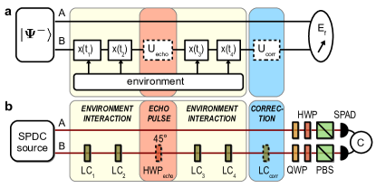
We investigated three different situations: a) the uncontrolled dynamics, where we simply look at the entanglement degradation resulting from the noisy channel; b) the controlled dynamics where we show how accessing classical information on the environment allows to operate corrections which fully restore the entanglement, and c) the echoed dynamics where entanglement is recovered by a simple local operation with no need to have access to the classical information.
Uncontrolled dynamics.– The reduced dynamics of induced by noise is in this case unambiguously described by the quantum ensemble , where stands for the joint probability and
| (3) |
with the overall phase accumulated up to step . As a result, each state of the ensemble is maximally entangled, so that also the average entanglement (2) is maximum for any : . However, the entanglement (1) of the average state, , exhibits quite a different behavior. The system concurrence for the uncontrolled dynamics decays with : in the case (full correlations), theory gives . For the concurrence, though more involved (see Appendix), shows a similarly decaying behavior. In the experiment we measured the entanglement obtained for three different values of with the generated sets of random phase sequences . For , the LCi with are set at a constant phase instead of . The experimental (black symbols) and theoretical results (black lines) are presented in Fig. 2. These results show that the system entanglement decreases as the accumulated phase grows.
Corrected dynamics.– In this case, we know the induced noise (since we generate it), and we can compensate it. Indeed, all that is needed is to insert another LC (LCcorr) after the channel and to apply to it a voltage so as to produce a phase , see Fig. 1. In practice, having only four LCs available, we used LC4 as the correction step and set it at a phase . For such corrected dynamics the initial state is fully recovered, together with its entanglement: , for any , see blue symbols (experiment) and blue lines (theory) in Fig. 2. This demonstrates that the channel-induced degradation of entanglement is only due to a lack of classical knowledge: once is known, entanglement is recovered by a local phase-shift operation.
Echoed dynamics (open-loop control).– Accessing information on the environment is not possible in practice in real quantum networks, where noise sources correspond to a large number of uncontrollable environmental degrees of freedom. Nevertheless, an open loop scheme operated by local control may still allow to recover the entanglement. To demonstrate this we use a control technique introduced in NMR Schlichter92 : just after the step , we apply a local bit-flip operation () on photon , which flips its polarization: and , see Fig. 1 a. Experimentally we insert a half-wave plate at between LC2 and LC3 when measuring the entanglement at , see Fig. 1 b. Our purpose is to induce an entanglement echo in the system dynamics. The state (3) which describes the system in each run of the experiment for now reads:
| (4) |
The local pulse is equivalent to a change of sign of the phases acquired at steps , and it may tend to cancel the effect of if the four phases are to a certain extent correlated. In general the echo pulse is expected to favor the recovery of the average state entanglement, especially for an environment with non-Markovian correlations.
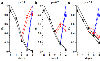
The plots in Fig. 2 show that, indeed, the entanglement for the echoed dynamics starts to increase at , see red symbols (experiment) and red lines (theory). It is also clear that entanglement recovery strongly depends on correlations. For (Fig. 2 a), the characteristic time scale of the environment dynamics is much larger than that of the system dynamics. In this case full entanglement recovery is possible: and we have that (red line), see Appendix. Partial recovery is possible when (Fig. 2 b for and Fig. 2 c for ). In that case, cancels only partially, and we have to deal with a bit more involved expression for the concurrence (red lines), see Appendix. Let us stress that, whereas in the corrected dynamics we used the knowledge of the sequence to cancel the accumulated random phase, in the echoed dynamics the (partial) cancellation of the phase needs no knowledge of the environment.
Our experimental data reported in Fig. 2 show a very good entanglement recovery, both for the corrected and the echoed dynamics. Deviations from the ideal expectations are mainly due to the imperfect preparation of the input state: in Fig. 2 we also plot (dashed lines) the expected entanglement for a mixed input state with a (measured) fidelity to the ideal input state , see Eqs. (10) and (11) in Appendix. Black and red dashed lines refer respectively to the uncontrolled and echoed entanglement, which are derived from Eqs. (18) and (19) in Appendix. For the corrected dynamics (blue squares), the recovered entanglement at step does not quite reach the initial entanglement at , this is due to the finite precision we have on setting the phases for each LC.
.4 Closed-loop control
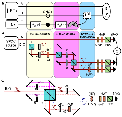
In this second experiment, qubits and are still encoded in the polarization of photons and , the environment being now a third qubit , encoded in the longitudinal momentum degree of freedom (the path) of photon . The state of can be either "up", , or "down", , see Fig. 3. The system plus environment is initially prepared in the state
| (5) |
The interaction of with the environment is engineered as follows: is first rotated by the gate , where and ; subsequently, undergoes the CNOT gate , which may flip the polarization of according to the state of , see Fig. 3 a. The gate is experimentally implemented by a balanced beam-splitter and an attenuation filter in both its output ports, with a ratio between their respective intensity transmission coefficients; the CNOT gate is implemented by an half-wave plate at in the "down" path of photon , see Fig. 3 b.
Uncontrolled dynamics.– The state of after the interaction is:
| (6) |
where is another Bell state. After tracing out the environment, the system is described by , with concurrence . No further operation is applied on before we measure the entanglement of . The corresponding entanglement of formation depends on , exhibiting a monotonous decay in the range , see the black curve (theory) and points (experiment) in Fig. 4 a.
Controlled dynamics.– We show how it is possible to recover entanglement by a "closed-loop" like control scheme. It consists of two steps: 1) after the gate , is projectively measured in the basis , and 2) depending on the outcome , a unitary operation is performed on , and , see Fig. 3 a. Experimentally, the selection of the measurement basis is obtained by a Mach-Zehnder interferometer with a variable phase which realizes the rotation , see Fig. 3 b. The unitary is obtained by doing nothing further on the output path and inserting a half-wave plate at in the path . The entanglement in is measured by mixing the polarization tomography data obtained on both output paths. Note that we actually used a folded version of the set-up presented in Fig. 3 b, see Appendix and Fig. 3 c.
The fact that we can distinguish the modes emerging from the second interferometer, allows to associate on a physical basis the ensemble (see Appendix) to the state of the system. Moreover, we tag the actual state of the ensemble during each run of the experiment. This classical information enables us to apply some suitable local control which depends on the actual state. The goal is to obtain a new quantum ensemble (see Appendix), whose corresponding density matrix, , exhibits the average entanglement of .
We investigate two special cases. First we take (the measurement basis of is thus its natural basis), yielding the quantum ensemble . For it we have for any value of . This entanglement is restored by the local control which flips the photon polarization each time the system is the state . This produces the output state , whose concurrence . We plot the corresponding entanglement obtained after the control loop as a function of in Fig. 4 a, see violet line (theory) and triangles (experiment): the restoration of the initial entanglement is achieved for any value of when the measurement basis angle is . As a second example, we consider the case in which the entanglement for the uncontrolled dynamics vanishes, which happens for . We show that the amount of entanglement recovery depends on the measurement performed on , that is to say on the angle of the rotated measurement basis. This measurement selects the system quantum ensemble (see Appendix). For it we find , since the concurrence of both states is . The measurement by itself does not produce any effect on the entanglement, which is vanishing for any in that case, see black line (theory) and points (experiment) in Fig. 4 b. Instead application afterwards of the local control on the qubit may lead to recovery of the average entanglement of the ensemble, . Indeed, the resulting output state for is
| (7) |
whose concurrence is , see the pink line (theory) and triangles (experiment) in Fig. 4 b. Here we see that the natural basis of is the optimal measurement basis to recover the entanglement, whereas for no entanglement is regained.
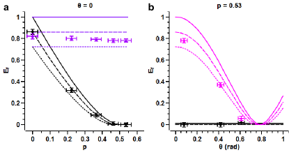
The experimental data (symbols) plotted in Fig. 4 show some deviation from the ideal expectations (continuous line). To explain them, we take into account the imperfect state preparation by our SPDC source: we also plot on Fig. 4 the expected entanglement for a mixed input state whose fidelity with the ideal input state is (dotted line) or (dashed line), see Appendix.
Conclusion
In this article we have presented two experiments showing that recovery of entanglement after the interaction of the members of an entangled state with a local non-Markovian environment can be achieved on-demand through local operations only. In the first experiment, the local environment is classical and induces low frequency noise, so that entanglement may be recovered by a local echo pulse. In the second experiment, the environment is a small quantum system (here a qubit) accessible to measurement, whose output controls a subsequent local operation on the system: as a result, entanglement recovery is obtained.
We note that in the second experiment there exists a measurement basis that selects system states with the largest amount of average entanglement. This maximum entanglement, recovered by the subsequent local operation, is known as entanglement of assistance divincenzo ; verstraete , a concept of which we provide here an experimental illustration. Instead the first experiment is a prototype of situations where the environment is not accessible in practice, typically because a large number of uncontrolled degrees of freedom are involved. Nevertheless, the recovery of entaglement by local operations is possible, since entanglement is not actually destroyed, but rather hidden due to a lack of classical information about which element in an ensemble of entangled states we are dealing with darrigo2014Annals .
Interestingly, the scheme of our first experiment is the simplest instance of recently proposed architectures, which should limit the detrimental up-scaling hardware-intrinsic decoherence, namely networks of smaller mutually entangled subsystems. Striking examples are trapped ions where modes in a single trap become dense as the trap becomes larger, acting as stray degrees of freedom, besides exquisitely solid-state systems as electrostatically defined quantum dots, silicon-based implanted impurities and optically active dopants ladd2010 . Very effective on-demand recovery by local operations is possible when noise has strong low-frequency components. We stres that this is a very relevant physical case, noise being a major drawback for solid state quantum computation PaladinoReview2013 ; ladd2010 , and it is likely to be an important source of decoherence in practical computation and communication networks. Direct applications of the scheme of our second experiment can be also envisaged in cavity quantum electrodynamics (QED) haroche2006 ; ritter2012 or in circuit QED systems wallraff2012 , where two-level quantum systems are strongly coupled to discrete photon modes in high-quality cavities. Finally we remark that this work, besides experimentally demonstrating novel physics related to non-Markovianity of open quantum systems, namely entanglement recovery by local operations, envisages new applications of quantum control techniques ithier2005PRB ; cook2007 ; bylander2011NatPhys ; Vijay2012 ; Murch2013 to distributed architectures.
Acknowledgements
G.B. acknowledges support from MIUR-PRIN 2011. P.M., F.S. and A.O. acknowledge support from the European project QWAD, Quantum Waveguide Application and Devices, http://www.qwad-project.eu/. R.L.F. acknowledges support by the Brazilian funding agency CAPES [Pesquisador Visitante Especial-Grant No. 108/2012]. A.d’A and R.L.F. acknowledge support from Centro Siciliano di Fisica Nucleare e Struttura delle Materia (Catania).
Appendix
.5 Entanglement of formation
As entanglement measure we use the entanglement of formation PlenioReview ; HorodeckiReview , which can be directly obtained from the concurrence wootters1998PRL by the following formula:
| (8) |
where and . Here () are the square roots of the eigenvalues of the non-Hermitian matrix , being the conjugate of .
.6 Open-loop control
Random phases.– The random variables are Gaussian with a standard deviation and an average , being the ensemble average. Since we disposed of half-wave LCs, which could only generate phases in , this setting provided that of the random phases were inside the experimentally achievable interval. Each sequence of random variables were generated (using Scilab random number generation function "grand") by keeping equal to with probability and independent from with probability .
The degree of memory in may be quantified by , which corresponds to the correlation coefficient Papoulis1965 between and inside each sequence:
| (9) |
Imperfect initial state.– To take into account the effect of the imperfect state generated by our SPDC source, we consider the following partially mixed state as input sate:
| (10) |
where input state is the maximally mixed input state and the mixing parameter is related to the fidelity by
| (11) |
Theoretical calculation of the entanglement.– We calculate the output state of the two-photon system when the initial state is .
For the uncontrolled dynamics, the two-photon state averaged on is:
| (12) |
where is given by Eq. (3). We will use the following abbreviations: where and . The noise only affects the coherences . These coherences are calculated by averaging the phase factor :
| (13) |
whose explicit expressions are:
| (14) |
For the echoed dynamics, we have to replace in Eq. (12), for , with from the state (4). We call the new average state. The only non-trivial element we have to calculate is
| (15) |
whose explicit expressions are:
| (16) |
By means of the equations (14), (16) and by taking into account that the considered noisy channel is unital (the channel does not change the input state ), it is straightforward to calculate the corresponding output state for the initial state (10), simply by using the linearity of quantum operations.
The system concurrence can be calculated by the formula
| (17) |
since the density matrix assumes always a X-form yu2007QIC . In the case of uncontrolled dynamics, the concurrence reads
| (18) |
with , whereas in the case of echoed dynamics, the concurrence is given by
| (19) |
with . Obviously, for we obtain the formula relative to the perfect state preparation . From (18) and (19), we can derive the entanglement of formation by means of Eq. (8).
.7 Closed-loop control
Actual experimental set-up.– The actual set-up that was implemented for this second experiment is shown in Fig. 3 c. For the sake of phase-stability and convenience, we opted for a folded version of the set-up shown in Fig. 3 b: the two Mach-Zehnder interferometers were replaced by two Sagnac interferometers using a single beam-splitter. Likewise, we chose to measure the exit modes "" and "" on the same exit port "": for a given angle , "" was measured for and "" was measured for .
Ensembles of pure states.– In the ensemble of pure states , , , and . With regard to the quantum ensemble , we have and . For the ensemble , and .
Imperfect state preparation.– To take into account the imperfection of the state preparation (originating from the SPDC source and the CNOT wave plate mainly), we modeled the initial state as in Eq. 10. The fidelity of the initial state was comprised in the interval , it was estimated by measuring separately the fidelity of the and states in the "up" and "down" paths respectively. Note that in Fig. 4 a, the entanglement measured for is slightly lower than for (violet triangles) mainly because of the noise added by the CNOT on .
Theoretical calculation of the entanglement.– For the uncontrolled dynamics, when the input state is the mixed state given by (10), the output state has a concurrence:
| (20) |
For the controlled dynamics and the same input state, the output state has the concurrence:
| (21) |
Error bars.– The errors bars on Fig. 4 are calculated from the Poissonian statistical errors associated to the coincidence counts.
The vertical error bars stem from the propagation of the Poissonian statistical errors of the 36 coincidence counts used for the quantum tomography that allows to measure .
The horizontal error bars, for the measurements done varying (Fig. 4 a), stem from the Poissonian statistical errors of the coincidence counts used to set :
where and ( and ) are measured coincidence counts corresponding to the state on the path (to the state on the path ). The error on is thus given by:
where is the the Poissonian statistical error on .
The horizontal error bars, for the measurements done varying (Fig. 4 b), stem from the Poissonian statistical errors of the coincidence counts used to set :
where and ( and ) are the coincidence count values measured on the output mode (). The error on is given by:
References
- (1) Lunghi, T. et al. Experimental bit commitment based on quantum communication and special relativity. Phys. Rev. Lett. 111, 180504 (2013).
- (2) Ekert, A. & Renner, R. The ultimate physical limits of privacy. Nature 507, 1443 (2014).
- (3) Kimble, H. J. The quantum internet. Nature 453, 1023 (2008).
- (4) Sciarrino, F. & Mataloni, P. Insight on future quantum networks. PNAS 109, 20169 (2012).
- (5) Perseguers, S., Lapeyre, G., Cavalcanti, D., M, M. L. & Acín, A. Distribution of entanglement in large-scale quantum networks. Reports on Progress in Physics. Physical Society 76, 096001 (2013).
- (6) Xiang, Z.-L., Ashhab, S., You, J. Q. & Nori, F. Hybrid quantum circuits: Superconducting circuits interacting with other quantum systems. Rev. Mod. Phys. 85, 623–653 (2013).
- (7) Steane, A. M. Space, time, parallelism and noise requirements for reliable quantum computing. Fortschr. Phys. 46, 443 (1998).
- (8) Preskill, J. Reliable quantum computers. Proc. R. Soc. Lond. A 454, 385 (1998).
- (9) DiVincenzo, D. P. The physical implementation of quantum computation. Fortschr. Phys. 48, 771 (2000).
- (10) Ladd, T. D. et al. Quantum computers. Nature 464, 45 (2010).
- (11) Plenio, M. B. & Virmani, S. Title. Quant. Inf. Comput. 7, 1 (2007).
- (12) Horodecki, R., Horodecki, P., Horodecki, M. & Horodecki, K. Quantum entanglement. Rev. Mod. Phys. 81, 865 (2009).
- (13) Bennett, C. H. et al. Teleporting an unknown quantum state via dual classical and einstein-podolsky-rosen channels. Phys. Rev. Lett. 70, 1895 (1993).
- (14) Bouwmeester, D. et al. Experimental quantum teleportation. Nature 390, 575 (1997).
- (15) Boschi, D., Branca, F., De Martini, F., Hardy, L. & Popescu, S. Teleporting an unknown quantum state via dual classical and einstein-podolsky-rosen channels. Phys. Rev. Lett. 80, 1121 (1998).
- (16) Ursin, R. et al. Entanglement-based quantum communication over 144 km. Nature Physics 3, 481 (2007).
- (17) Gisin, N., Ribordy, G., Tittel, W. & Zbinden, H. Quantum cryptography. Rev. Mod. Phys. 74, 145 (2002).
- (18) Gottesman, D. & Chuang, I. L. Demonstrating the viability of universal quantum computation using teleportation and single-qubit operations. Nature 402, 390 (1998).
- (19) . Brukner, ukowski, M., Pan, J.-W. & Zeilinger, A. Bell’s inequalities and quantum communication complexity. Phys. Rev. Lett. 92, 127901 (2004).
- (20) Kmer, P. et al. A quantum network of clocks. Nature Physics 10, 582 (2014).
- (21) Bennett, C., DiVincenzo, D., Smolin, J. & Wootters, W. Mixed-state entanglement and quantum error correction. Phys. Rev. A 54, 3824 (1996).
- (22) D’Arrigo, A., Lo Franco, R., Benenti, G., Paladino, E. & Falci, G. Recovering entanglement by local operations. Ann. Phys. 350, 211 (2014).
- (23) Paladino, E., Galperin, Y. M., Falci, G. & Altshuler, B. L. noise: implications for solid state quantum information. Rev. Mod. Phys. 86, 361 (2014).
- (24) Vandersypen, L. M. K. & Chuang, I. L. Nmr techniques for quantum control and computation. Rev. Mod. Phys. 76, 1037 (2005).
- (25) Wiseman, H. M. & Milburn, G. J. Quantum Measurement and Control (Cambridge University Press, USA, New York, 2010).
- (26) Cohen-Tannoudji, C., Dupont-Roc, J. & Grynberg, G. Atom- Photon Interactions: Basic Processes and Applications (Wiley, New York, 1992).
- (27) Rivas, Huelga, S. F. & Plenio, M. B. Quantum non-markovianity: Characterization, quantification and detection. Rep. Prog. Phys. 77, 094001 (2014).
- (28) Bellomo, B., Lo Franco, R. & Compagno, G. Non-markovian effects on the dynamics of entanglement. Phys. Rev. Lett. 99, 160502 (2007).
- (29) Liu, B.-H. et al. Experimental control of the transition from markovian to non-markovian dynamics of open quantum systems. Nature Physics 7, 931–934 (2011).
- (30) Chiuri, A., Greganti, C., Mazzola, L., Paternostro, M. & Mataloni, P. Linear optics simulation of quantum non-markovian dynamics. Scientific Reports 2, 968 (2012).
- (31) Lo Franco, R., Bellomo, B., Andersson, E. & Compagno, G. Revival of quantum correlation without system-environment back-action. Phys. Rev. A 85, 032318 (2012).
- (32) Xu, J.-S. et al. Experimental recovery of quantum correlation in absence of system-envionemt back-action. Nat. Comm. 4, 2851 (2013).
- (33) Wang, Y. et al. Preservation of bipartite pseudoentanglement in solids using dynamical decoupling. Phys. Rev. Lett. 106, 040501 (2011).
- (34) Roy, S. S., Mahesh, T. S. & Agarwal, G. S. Storing entanglement of nuclear spins via uhrig dynamical decoupling. Phys. Rev. A 83, 062326 (2011).
- (35) Lo Franco, R., D’Arrigo, A., Falci, G., Compagno, G. & Paladino, E. Preserving entanglement and nonlocality in solid-state qubits by dynamical decoupling. Phys. Rev. B 90, 054304 (2014).
- (36) Wootters, W. K. Entanglement of formation of an arbitrary state of two qubits. Phys. Rev. Lett. 80, 2245 (1998).
- (37) Kwiat, P. G., Mattle, K., Weinfurter, H., Zeilinger, A. & Shih, A. V. S. Y. New high-intensity source of polarization-entangled photon pairs. Phys. Rev. Lett. 75, 4337 (1995).
- (38) Rivas, Á., Huelga, S. F. & Plenio, M. B. Entanglement and non-Markovianity of quantum evolutions. Phys. Rev. Lett. 105, 050403 (2010).
- (39) Schlichter, C. P. Principles of Magnetic Resonance 3ED (Springer-Verlag, Berlin, 1992).
- (40) DiVincenzo, D. et al. Lecture Notes in Computer Science 1509, 247 (1999).
- (41) Verstraete, F., Popp, M. & Cirac, J. I. Phys. Rev. Lett. 92, xxxx (2004).
- (42) Haroche, S. & Raimond, J. Exploring the Quantum (Oxford University Press, Oxford, 2006).
- (43) Ritter, S. et al. An elementary quantum network of single atoms in optical cavities. Nature 484, 195 (2012).
- (44) Wallraff, A. et al. Strong coupling of a single photon to a superconducting qubit using circuit quantum electrodynamics. Nature 431, 162 (2004).
- (45) Ithier, G. et al. Decoherence in a superconducting quantum bit circuit. Phys. Rev. B 72, 134519 (2005).
- (46) Cook, R. L., Martin, P. J. & Geremia, J. M. Optical coherent state discrimination using a closed-loop quantum measurement. Nature 446, 774 (2012).
- (47) Bylander, J. et al. Noise spectroscopy through dynamical decoupling with a superconducting flux qubit. Nature Phys. 7, 565 (2011).
- (48) Vijay, R. et al. Stabilizing rabi oscillations in a superconducting qubit using quantum feedback. Nature 490, 77 (2012).
- (49) Murch, K. W., Weber, S. J., Macklin, C., & Siddiqi, I. Observing single quantum trajectories of a superconducting quantum bit. Nature 502, 211 (2013).
- (50) Papoulis, A. Probability, Random Variables and Stochastic Processes (New York: McGraw Hill, 1965).
- (51) Yu, T. & Eberly, J. H. Evolution from entanglement to decoherence of bipartite mixed X states. Quantum Information and Computation 7, 459 (2007).