Simulations of cm-wavelength Sunyaev-Zel’dovich galaxy cluster and point source blind sky surveys and predictions for the RT32/OCRA-f and the Hevelius 100-m radio telescope.

Abstract

We investigate the effectiveness of blind surveys for radio sources and galaxy cluster thermal Sunyaev-Zel’dovich effects (TSZEs) using the four-pair, beam-switched OCRA-f radiometer on the 32-m radio telescope in Poland. The predictions are based on mock maps that include the cosmic microwave background, TSZEs from hydrodynamical simulations of large scale structure formation, and unresolved radio sources. We validate the mock maps against observational data, and examine the limitations imposed by simplified physics. We estimate the effects of source clustering towards galaxy clusters from NVSS source counts around Planck-selected cluster candidates, and include appropriate correlations in our mock maps. The study allows us to quantify the effects of halo line-of-sight alignments, source confusion, and telescope angular resolution on the detections of TSZEs.

We perform a similar analysis for the planned 100-m Hevelius radio telescope (RTH) equipped with a 49-beam radio camera and operating at frequencies up to 22 GHz.

We find that RT32/OCRA-f will be suitable for small-field blind radio source surveys, and will detect $33^{+17}_{-11}$ new radio sources brighter than $0.87\ \rm mJy$ at 30 GHz in a $1\ \rm deg^{2}$ field at $>5\sigma$ CL during a one-year, non-continuous, observing campaign, taking account of Polish weather conditions. It is unlikely that any galaxy cluster will be detected at $3\sigma$ CL in such a survey. A $60$-deg² survey, with field coverage of $2^{2}$ beams per pixel, at 15 GHz with the RTH, would find $<1.5$ galaxy clusters per year brighter than 60 $\mu$Jy (at $3\sigma$ CL), and would detect about $3.4\times 10^{4}$ point sources brighter than $1\ \rm mJy$ at $5\sigma$ CL, with confusion causing flux density errors $\lesssim 2\%\,(20\%)$ in 68% (95%) of the detected sources.

A primary goal of the planned RTH will be a wide-area ($\pi$ sr) radio source survey at 15 GHz. This survey will detect nearly $3\times 10^{5}$ radio sources at $5\sigma$ CL down to $1.3$ $\mathrm{mJy}$, and tens of galaxy clusters, in one year of operation with typical weather conditions. Confusion will affect the measured flux densities by $\lesssim 1.5\%\,(16\%)$ for 68% (95%) of the point sources. We also gauge the impact of the RTH by investigating its performance if equipped with the existing RT32 receivers, and the performance of the RT32 equipped with the RTH radio camera.

I Introduction

Dedicated wide-area and all-sky surveys over the next decade will boost our knowledge of large-scale structure formation, structure evolution, and cosmology. Optical galaxy redshift surveys such as LSST, EUCLID, and 4MOST will provide shapes and spectroscopic redshifts of millions of galaxies with redshift $z\lesssim 2$. The eROSITA X-ray survey will provide high angular resolution ($\lesssim 0.5^{\prime}$) maps and spectra of thousands of galaxy clusters. These optical and X-ray data will trace the expansion history of the Universe and probe the mass function of collapsed objects. This will constrain ‘dark energy’ (DE) and/or improve our understanding of gravity on the largest scales.

Wide area cm-wavelength radio surveys will complement these observations via measurements of the Sunyaev-Zel’dovich effects (Sunyaev & Zeldovich 1972) (hereafter SZE) from young galaxy clusters. SZE data can combine with other data to constrain cluster masses and abundances in redshift space. Radio catalogues with sub-mJy sensitivity will also provide a census of active galactic nuclei (AGN), showing their distribution and activity in relation to forming and evolving galaxies and clusters. Since inflation-based cosmological models typically predict non-Gaussian curvature perturbations, observations of the abundances of massive, high-redshift clusters provide a window into the very early Universe via constraints on the shape and the amplitude of the primordial non-Gaussianity imprinted in matter distribution (Dalal et al. 2008; Matarrese & Verde 2008).

Wide area radio source surveys also have the potential to test DE by measuring the expansion-driven decay of gravitational potential wells – the integrated Sachs-Wolfe effect (Sachs & Wolfe 1967) – detected by cross-correlation with the primary CMB at large scales (Afshordi & Tolley 2008).

Galaxy clusters as observationally useful tracers of Mpc-scale mass distributions have been used to constrain cosmological parameters (White et al. 1993; Eke et al. 1996; Komatsu & Seljak 2002; Voit 2005; Rapetti et al. 2010; Vanderlinde et al. 2010; Burenin & Vikhlinin 2012; Planck Collaboration et al. 2014b; Weinberg et al. 2013; Benson et al. 2013), local non-gaussianity of primordial density perturbations (Matarrese et al. 2000; Sadeh et al. 2007; Roncarelli et al. 2010) and departures from the standard cosmological model (Schmidt et al. 2009b, a; Dunsby et al. 2010; Ferraro et al. 2011; Wyman et al. 2014; Giannantonio et al. 2014). Clusters are also a promising source of information on the dark energy equation of state parameter in the standard $\Lambda$CDM model (Sehgal et al. 2011; Kneissl et al. 2001; Alam et al. 2011), and are crucial for attempts to solve the missing-baryon problem (Afshordi et al. 2007; Planck Collaboration et al. 2014a; Van Waerbeke et al. 2014). Cool-core clusters provide laboratories for studying interplay between processes such as star formation, AGN feedback, thermal emission, thermal conduction, plasma magnetisation, photoionisation and metallicity-dependent molecular line cooling (Voit 2011; Voit & Donahue 2014). The most effective means of finding galaxy clusters to date has been by X-ray detections of thermal emission from their hot intra-cluster medium (ICM). However, complementary information on the 3D-temperature distribution of ICM is also available through observations at radio frequencies(Prokhorov et al. 2011). With the advent of current and near-future blind radio surveys, thousands of new galaxy clusters will be found via measurements of their thermal Sunyaev-Zel’dovich effect (TSZE) at arcminute and sub-arcminute scales (Kneissl et al. 2001; De Petris et al. 2002; Vanderlinde et al. 2010; Sehgal et al. 2011; Planck Collaboration et al. 2011; Muchovej et al. 2012; Mantz et al. 2014). On such scales, and at the frequencies of tens of GHz at which most surveys are undertaken, unresolved radio sources are an important source of contamination and confusion (Vale & White 2006). From another point of view, the data on sub-mJy radio sources that will emerge from blind surveys is an important measure of the differential source count (Muchovej et al. 2010), another piece of useful cosmological information. Recent important catalogues in this class have come from the WMAP and Planck satellites, which have surveyed Jy-level sources over $3\pi$-sr, the 22-GHz Australia Telescope survey (Murphy et al. 2010), which gives nearly $2\pi$-steradians coverage with flux-density threshold of 40 mJy, the 15-GHz Ryle Telescope survey (Waldram et al. 2003), which provides the differential source count above $\sim 25$ mJy over $\sim 520$ $\mathrm{deg^{2}}$, and the SZA survey to sub-mJy levels at 31-GHz in selected fields with total area $7.7$ $\mathrm{deg^{2}}$ (Muchovej et al. 2010).

The OCRA-f radio array on the 32-metre telescope (RT32) in Poland is another facility capable of cm-wave surveys. OCRA-f is the successor to the OCRA-p single pair, dual beam, beamswitched radiometer (Browne et al. 2000). The two OCRA receivers were constructed by the University of Manchester. OCRA-f was designed to carry out targeted TSZE observations (Lancaster et al. 2011) and blind radio source surveys, and it is now about to start operation in small northern sky regions. In the future the OCRA-f technology could be developed into a wide-field, wide-band, multi-beam radio camera for the Polish 100-m radio telescope Hevelius (RTH) that is currently being planned. The RTH project was signed into the Polish Roadmap for Research Infrastructures in 2011. It has received strong scientific support from the European VLBI Network Consortium, and funding from the European Regional Development Fund will be decided in the near future. It is expected that the RTH will carry out blind, large-area, radio surveys to mJy flux density levels at frequencies around 15 GHz.

Bearing in mind the importance of the TSZE for cosmological studies, it is timely to investigate the possibility that RTH and RT32/OCRA-f could find clusters in blind surveys, and to examine the quality of the radio source counts that would result from such surveys. This investigation is the main purpose of this paper.

Proper calibration and radio map reconstruction from survey data will require excellent knowledge of the instrumental beams, the noise properties of the radiometers, and the intervening foregrounds, including the effects of atmospheric emission and absorption. Simulations of atmospheric and receiver effects are in progress, but in the present paper we focus on models of the centimetre-wavelength radio sky. We have two main objectives: (i) to create reliable, calibrated, mock maps of the astrophysical signals to be sought for in the planned surveys; and (ii) to predict the number of objects that are likely to be found in these surveys. This work can be used to inform specifications for future RT32 and RTH receivers. More specifically, for an assumed survey geometry and duration we will estimate the number of radio sources that will be detected, the likely flux density threshold, and the ability of the systems to detect the TSZEs from galaxy clusters. These results, combined with realistic simulations of atmospheric foregrounds and receiver performance (Lew 2015, in preparation), will provide tests of the astrophysical signal reconstruction procedures that will be applied to the real data at the map-making stage.

The structure of this paper is as follows. In section II we outline the instrumental properties. In section III we describe simulations of cosmic microwave background (CMB) intensity fluctuations, the TSZEs, and the point source population. In section IV we test our hydrodynamic simulations against available observational data and scaling relations resulting from realistic high-resolution simulations of galaxy clusters. The main results are gathered in section V. We discuss these results and conclude in sections VI and VII.

II RT32 and RTH instruments

We derive predictions for the expected point source and galaxy cluster detection rates principally for two instruments, the OCRA-f receiver installed on the 32-m radio telescope in Poland (hereafter RT32), and the planned 49-beam receiver for the 100-m radio telescope Hevelius (RTH), which is planned for construction starting in 2017. We highlight the impact of telescope and receiver size by also predicting the survey outcomes with the receivers swapped between the telescopes. For the 49-beam system we consider survey performance in three sub-bands around 15 GHz. We also calculate predictions for the existing 22-GHz RT32 receiver, since the planned 30-GHz RT32 survey will be conducted with this receiver taking data in parallel with OCRA-f. Again, we compare the effect of surveying with the same 22-GHz receiver on the RTH. In this section we outline the basic instrumental parameters of the three receivers.

II.1 The OCRA-f receiver

OCRA-f is a 30-GHz, four-pair, beam-switched, secondary focus, receiver array installed at the fully-steerable, 32-metre, Cassegrain radio telescope in Toruń (Poland). The receiver pairs are identical and run independently. In simple terms, the receiver operates as follows. Signals from the two arms of each receiver pair are mixed in a $90^{\circ}$, four-port Lange coupler and amplified at cryogenic temperatures in first-stage low-noise amplifiers (LNAs). Next, they are phase shifted by $180^{\circ}$, mixed again, in a second, identical, $90^{\circ}$ coupler, and amplified in second-stage room-temperature amplifiers. The resulting signal is passed to a square-law detector, filtered, amplified in video-amplifiers, and digitised in an analog-to-digital data acquisition card installed in a PC-class computer.

The technical design and laboratory tests of individual OCRA-f components have been described in Kettle & Roddis (2007) and also in Peel (2010). By design OCRA-f mitigates fluctuations in atmospheric radio power by differencing the total power signals detected in the two arms of the receiver, which view slightly different directions on the sky through corrugated feeds. The observable cm-wavelength signals from astrophysical sources are contaminated by atmospheric emission (and reduced by variable atmospheric absorption), mostly from water vapour and water droplets (in clouds). These signals fluctuate in time and space due to the turbulent nature of atmospheric flows. The single difference mitigates these fluctuations because the near-field telescope beams largely overlap at the altitudes of clouds. Internal gain instabilities in the receiver are mitigated by differencing pairs of single difference signals phase shifted with respect to each other by $180^{\circ}$. Phase switching (between $0^{\circ}$ and $180^{\circ}$) is introduced at a rate which is adjustable up to a few kHz. In its design and operation, each OCRA-f receiver pair is similar to the receivers used by the WMAP satellite.

In preparation for the planned surveys we numerically simulate the whole receiver chain. This allows us to generate realistic time-domain noise, and to test map reconstruction techniques that can cope with non-uniform and incomplete sky coverage (Lew 2015, in preparation). For the purpose of the present work, the details of these simulations can be characterised by a few parameters describing the system noise and antenna sensitivity. These are estimated based on in-lab measurements, or astronomical calibrations, and are gathered in table 1.

Details of the data preparation and reduction pipelines that will lie behind map-making and signal reconstruction from the raw data are beyond the scope of the present work and will be discussed separately. Here we note only that the raw data from each OCRA-f detector, as well as from the K-band receiver, are digitised at an adjustable rate – typically about $10^{5}$ samples per second per data channel. The data are time-tagged according to a 1-second pulse signal from a hydrogen maser. Next, they are averaged within a switching state, and the double-difference (DD) is calculated and referenced to sky coordinates by linear interpolation from the RT32 pointing datastream. At the end of this real-time process, the DD data are samples with time resolution compatible with the switching time, which is typically set to 3 ms, so that fast-scanning strategies are supported. Occasional calibration pulses are injected into a single switching state, so as to appear in the DD data, and absorber on-off sequences are introduced periodically during the scan to track the stability of the calibration diode. Prototype map-making and source-extraction pipelines are currently being tested using simulations of the astronomical sky and the sources of noise: the astrophysical part of these simulations is described in the present paper.

Over the last few years RT32 control, OCRA-f data acquisition, and the data processing pipelines have been developed and improved to provide good calibration and to support sky-scanning strategies that can optimise between field size, scan completeness, and the elevation-dependence of atmospheric and astronomical signals.

II.2 A 100-metre Hevelius radio telescope

The construction of a fully-steerable, $\sim 100$-m, radio telescope is based on a number of science projects, but its operation will be centred on an all-purpose radio camera, providing 49 broad-band horns, with four 2-GHz bands per channel, and full polarisation, for a total of 784 independent data channels. The polarisation and spectroscopic data from all horns will be recorded at high time resolution. The large collecting area of the primary antenna and wide instantaneous frequency coverage ($6-22$ GHz) will result in high sensitivity, and the multiple feeds will provide a wide instantaneous field of view (FOV), allowing for effective mitigation of atmospheric foregrounds and fast sky mapping. It is expected that the analyses of OCRA-f simulations and data acquired from its early observations will provide software pipeline that will be readily adapted to the data from the RTH.

The preferred location of the RTH is deep within a forested part of a natural reserve in northern Poland. This site is sufficiently remote that the present-day radio frequency interference (RFI) environment is benign, and this should persist several decades into the future, even with increasing urbanisation and density of telecommunications signals.

It is anticipated that the RTH will be an instrument uniquely suitable for wide-area, blind, radio surveys in the frequency ranges accessible to ground-based, sea-level radio astronomy. Its operations will be constrained mostly by the typical weather conditions in eastern Europe, which dictate the high-frequency limit for effective operation, and define the fraction of the year for which sensitive observing is possible. In addition to its stand-alone capabilities, RTH will provide a dramatic enhancement to the European Very Long Baseline Interferometry Network (EVN), and open new opportunities for the international scientific community to carry out a wide range of radio observations including: (i) molecular studies of star-forming regions and circumstellar envelopes; (ii) searches for new molecules in the interstellar medium and solar system objects; (iii) measurements of the redshifted, 115-GHz emission line of ${}^{12}\mathrm{C}^{16}\mathrm{O}(1-0)$ from sources with redshift of $z\gtrsim 4.2$; (iv) blind surveys for discrete sources; (iv) continuum surveys of Galactic emission; (v) measurements of the Sunyaev-Zel’dovich effect in galaxy clusters; (vi) observations of transient sources; and (vii) studies of radio pulsars.

An important scientific goal for the planned telescope is a new radio survey, at around 15 GHz, that will detect and characterise the spectra of a few $\times 10^{5}$ radio sources in the northern hemisphere down to mJy flux densities (point iv above). Combinations of different but overlapping field sizes will result in tiered surveys of varying depths limited only by source confusion, and, potentially, the detection of new TSZEs. The most important parameters of the RTH and the 49-beam receiver are collected in table 1.

Table 1: Selected parameters of the 32-m and the planned 100-m radio telescopes and their receivers. We compare the existing K- and Ka-band receivers installed on the 32-metre telescope in Toruń with the 49-receiver array of the RTH. We highlight the effect of antenna size by including the performance that would be expected if the existing receivers were to operate on the 100-m telescope, or the radio camera was to be sited on the RT32.

	32-m radio telescope (RT32)			100-m Hevelius radio telescope (RTH)
Location [dms]	$18^{\circ}\,33^{\prime}\,50.6^{\prime\prime}\,\mathrm{E},\,53^{\circ}\,05^{\prime}\,43.7^{\prime\prime}\,\mathrm{N}$			$18^{\circ}\,21^{\prime}\,42^{\prime\prime}\,\mathrm{E},\,53^{\circ}\,39^{\prime}\,32^{\prime\prime}\,\mathrm{N}$
Aperture [m]	32	32	32	100	100	100
Geometric area [$\mathrm{m}^{2}$]	804	804	804	7854	7854	7854
Surface rms error [mm]	$\sim 0.6$	$\sim 0.6$	$\sim 0.6$	0.5	0.5	0.5
Band name	Ku	K	Ka	Ku	K	Ka
Central frequency [GHz]	15	22	30	15	22	30
Technology	HEMT/MMIC radiometers
Bandwidth [GHz]	6	4	8	6	4	8
Wavelength [cm]	2.00	1.36	1.00	2.00	1.36	1.00
HPBW ($\theta_{b}$) [′]	2.46	1.68	1.23	0.79	0.54	0.39
$\Omega_{B}$ [$10^{-7}$ sr]	5.81	2.70	1.45	0.59	0.28	0.15
Surface efficiency	$0.42^{+0.07}_{-0.06}$	$0.35^{+0.06}_{-0.05}$	$0.26^{+0.05}_{-0.04}$	$0.44^{+0.07}_{-0.07}$	$0.40^{+0.06}_{-0.06}$	$0.33^{+0.05}_{-0.05}$
Effective area [$\mathrm{m}^{2}$]	337	282	212	3479	3102	2592
Sensitivity ($\Gamma$) [K/Jy]	$0.12^{+0.02}_{-0.02}$	$0.10^{+0.02}_{-0.02}$	$0.08^{+0.01}_{-0.01}$	$1.26^{+0.20}_{-0.20}$	$1.12^{+0.18}_{-0.17}$	$0.94^{+0.15}_{-0.15}$
$T_{\mathrm{rec}}$ [K]	16	16	30	16	16	30
$T_{\mathrm{atm}}(z=0^{\circ},\mathrm{Jun})$ [K]	8	31	17	8	31	17
$T_{\mathrm{atm}}(z=0^{\circ},\mathrm{Dec})$${}^{[}^{]}$ [K]	7	16	13	7	16	13
$T_{\mathrm{sys}}(z=0^{\circ})$ [K]	24	47	47	24	47	47
Air mass $z=(30^{\circ},60^{\circ})$	$(1.15,2.00)$	$(1.15,2.00)$	$(1.15,2.00)$	$(1.15,2.00)$	$(1.15,2.00)$	$(1.15,2.00)$
$T_{\mathrm{sys}}(z=45^{\circ})$ [K]	$28^{+5}_{-4}$	$60^{+18}_{-25}$	$54^{+10}_{-10}$	$28^{+5}_{-4}$	$60^{+18}_{-25}$	$54^{+10}_{-10}$
Number of receivers	49	1	4	49	1	4
RMS noise [$\mathrm{mK/s}^{1/2}$],	$0.36^{+0.06}_{-0.05}$	$0.94^{+0.27}_{-0.40}$	$0.86^{+0.16}_{-0.16}$	$0.36^{+0.06}_{-0.05}$	$0.94^{+0.29}_{-0.40}$	$0.86^{+0.16}_{-0.16}$

III Simulations

We perform simulations within the framework of the standard $\Lambda$CDM cosmological model with cosmological parameters

$$\{\Omega_{b0},\Omega_{m0},\Omega_{\Lambda 0},n_{s},\sigma_{8},h\}=\{0.0463,0.279,0.721,0.972,0.821,0.7\}$$ (1)

which are compatible with the nine-year WMAP data (Hinshaw et al. 2013). For a scale-free primordial power spectrum this setup implies the amplitude of the scalar comoving curvature perturbation $\Delta_{\mathcal{R}}^{2}=2.405\cdot 10^{-9}$. While the Planck (CMB+lensing) estimates on $\sigma_{8}$ are slightly higher (Planck Collaboration et al. 2014a), this will not significantly alter our main results. We do not address the reported tension between the calibrations of the matter power spectrum inferred using high-redshift (CMB) and low-redshift (cluster) data (Planck Collaboration et al. 2014c), and henceforth assume the CMB-calibrated cosmology (see section VI for discussion of the anticipated impact of a slightly modified value of the $\sigma_{8}$ parameter).

III.1 Large scale structure simulations

We used a publicly-available version of the smooth particle hydrodynamics (SPH) code Gadget-2 (Springel 2005) to simulate large scale structure evolution in the past light cone. All calculations were carried out on the 2048-CPU shared memory supercomputer at the Poznań Supercomputing and Networking Centre. We created a number of large scale structure simulations that we stacked together in comoving space in order to generate a deep field of view that mimics the observational fields to be scanned in the planned surveys. For the primary results we generated 11 simulations, each of which contains $N_{\rm{CDM}}=512^{3}$ dark matter and $N_{\rm{gas}}=512^{3}$ gas particles within a comoving volume of $512^{3}\mathrm{Mpc}^{3}$. The simulations were recorded at 12 evolutionary stages, covering redshift range $z\approx(0.06,2.25)$. We used comoving gravitational softening lengths of 15 kpc/$h$ for CDM and baryon particles, and a mesh grid of size of $M=N^{1/3}$ was used for long-distance gravity force computations. The initial conditions were generated with the N-GenIC program (Springel 2003) working within the Zel’dovich approximation (Zel’dovich 1970), at an initial redshift $z_{\mathrm{ini}}=50$. The gas temperature at the initial redshift was calculated using the mean value between the coupled and adiabatic cases (Shapiro et al. 1994), $T_{\mathrm{ini}}\approx 73\,\mathrm{K}$. The CDM and gas particles masses are $M_{\rm{CDM}}\approx 2.2148\cdot 10^{10}M_{\odot}h^{-1}$, and $M_{\rm{gas}}\approx 0.4407\cdot 10^{10}M_{\odot}h^{-1}$. The simulations together contain nearly 3 billion particles and cover comoving volume $V_{\mathrm{tot}}\approx 1.476\,\mathrm{Gpc}^{3}$.

In order to test the stability of our results and to understand their sensitivity to variations of key parameters, we created a number of smaller test simulations, altering the selected parameters such as the initial redshift $z_{\mathrm{ini}}=\{50,100\}$, mass resolution (number of particles for a fixed comoving simulation volume) $N^{1/3}=\{128,256,512\}$, gravitational softening length $\{66,33,15,5\}$ kpc/$h$, number of neighbours used for smoothing length calculations (multiple values $N_{\mathrm{neig}}$ between $5$ and $66$), initial condition generator (N-GenIC and Grafic++), and cosmological parameter $\sigma_{8}$. The details of these tests are beyond the scope of the current paper, but we found that our central choice is both stable and in good agreement with observational data. The consistency checks that we made are described in Section IV.

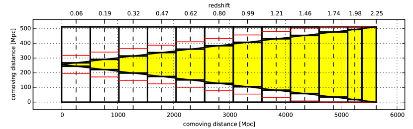
Figure 1: Deep field geometry: the $z$-$y$ plane. The horizontal, $z$, axis represents field depth and the vertical axis represents the $y$ coordinate. The $x$ coordinate, which is orthogonal to $y$ and $z$, is suppressed. The heavy black boxes indicate adjacent simulation box cubes. The shaded (yellow) rectangles represent slices used to approximate the past light cone for an observer located at $(x,y,z)=(L/2,L/2,0)$ where $L=512$ Mpc is the length of the side of the simulation box. Vertical dashed lines indicate the redshifts at which simulations were recorded. The horizontal red lines represent the 5-Mpc margin (expanded by a factor of 10 for visualisation) that define the cut-away domain used in SPH interpolations. The opening angle of the field of view in the assumed flat geometry is $\sim 5.2^{\circ}$.

Every deep field realisation consists of 11 simulation boxes stacked as shown in figure 1. Since the selected field of view cuts only about a third of the total simulation volume, in different FOV realisations we introduce random permutations of the simulation box ordering, apply random coordinate switches between $y$-$z$ and $x$-$z$, and apply random periodic particle shifts in three dimensions within the simulation box. These operations make better use of the total simulation volume and so allow better assessment of cosmic and sample variance, although the resulting samples are not entirely independent.

As explained in the caption of figure 1, we define a “slice” as a parallelepiped cut-away region corresponding to the inside of the shaded rectangles in figure 1 (marked in yellow). The actual region used for the SPH interpolations (see section III.2) is larger in the $x$-$y$ directions as indicated by the red lines in the figure. We refer to this larger region as a “domain”. Some particles within domains influence the density estimates inside the associated slice.

We use slice depths of 512 Mpc (the full size of the simulation box) in the $z$-direction. Our methodology allows us to use arbitrarily smaller values, which would result in a larger number of domains, but would also require more simulation snapshots to sample fully the evolution of the density field. Our choice causes the most distant simulation box, at the high-redshift extreme of the light cone, to contain at least two slices.

III.2 Galaxy clusters: search and properties

We run a Friends-of-Friends (FOF) algorithm with linking length parameter $b=0.2$ to identify groups of particles either in the hypersurface of the present for the whole simulation volume or as observed on the light cone, on a box-by-box. The corresponding comoving linking length, $L_{l}=b\langle l_{pp}\rangle$, depends on the mean inter-particle separation, $\langle l_{pp}\rangle$, which we crudely approximate as $\langle l_{pp}\rangle=(V/N)^{1/3}$ where $N$ is the total number of particles of a given type and $V$ is the simulation volume. The search for halos is done using both CDM and gas particles, and we require halos to contain at least $N_{h}=600$ particles. This number typically corresponds to halo mass $>M_{h,\rm min}\approx 1.3\cdot 10^{13}M_{\odot}h^{-1}$. $M_{h,\rm min}$ depends on gas mass fraction, and so slowly evolves during cluster formation. This is because halos are defined in terms of the FOF linking length and slightly different ratios of gas to DM particles can appear in halos of the same $N_{h}$, depending on their merging history.

At our mass resolution, galaxy-cluster-sized halos are resolved with tens of thousands of particles. The most massive systems, with halo masses $M_{h}>2\cdot 10^{15}M_{\odot}h^{-1}$, are comprised of $N_{h}>1.6\cdot 10^{5}$ particles. We find tens of thousands of galaxy-group or galaxy-cluster size halos in each deep-field simulation, out to the limiting redshift that we used, $z_{\rm max}=2.25$. For each identified halo we calculated a set of properties including location in the comoving space, peculiar velocity, velocity dispersion, redshift corresponding to comoving distance (which typically does not exactly correspond to the redshift resulting from the stage of evolution), kinetic and potential energies, angular size, gas mass fraction, shape parameters (such as eccentricity), the location of the gravitational potential minimum, the mass centre, etc. In order to test halo properties at certain overdensity thresholds we reconstruct the three-dimensional (3D) distributions of mass density, gas temperature, and gas density-weighted temperature using SPH interpolations (see section III.3) on a regular grid that resolves the halo and maintains a guard region of adjustable size around it. For all halos we use a constant grid resolution of 50 kpc (comoving), which we find sufficient at our mass resolution. The innermost regions of galaxy clusters (with overdensities above 2500) are not well resolved, but in that regime our adiabatic simulations are also deficient. In this paper we are concerned with regions of much lower overdensity, $\delta=\{\mathrm{vir},200,500\}$ (see below). Using the 3D distributions we reconstruct direction-averaged radial profiles of (i) overdensity (with respect to the critical density of the Universe at the corresponding redshift); (ii) mass; (iii) temperature; and (iv) gas mass fraction. We use these functions to derive the halo properties at the selected overdensity thresholds.

The radial distance from the halo centre for a chosen overdensity ($r_{\delta}$) and the corresponding quantities calculated at that distance are sensitive to the choice of centroid. We define the halo centroid as the location of the minimum of the gravitational potential derived from the halo SPH particle distribution. Profiles are calculated with respect to that point because it is much more stable to the presence of sub-halos than, for example, the mass centroid. We make an exception for the integrated Compton Y-parameter $Y^{\mathrm{INT}}$ (Eq. 12) which we always calculate within $r_{\delta}$ of the maximum of the line-of-sight integrated, two-dimensional (2D), map of the Compton $y$-parameter, since this matches the way that observers measure $Y^{\rm INT}$.

Throughout this paper we denote “virial” quantities (such as virial radius $r_{\mathrm{vir,c}}$) by subscript “vir” which formally corresponds to overdensity $\delta_{\mathrm{vir}}\approx 100.2$ calculated for the assumed cosmological parameters at the lowest considered redshift of ($z=0.06$) (Eke et al. 1998) and with respect to the critical density as usually indicated by subscript “c”. Throughout this paper we work only with overdensities calculated with respect to the critical density of the Universe at the measurement redshift and henceforth we will skip the explicit subscripting with “c”.

The details of the halo finder used are irrelevant for our main results, but our choice of the FOF algorithm allows us to generate a relatively high-resolution (compared to the size of the simulation) grid with SZE relevant quantities (such as density weighted temperature). The fact that FOF binds multiple halos into a single system (be it gravitationally bounded or not) does not worsen the resolution since we use a fixed resolution for all halos. The definition of what constitutes a halo (i.e., details of the criteria for finding a halo) may have some impact on the scaling relations constructed for selected overdensity thresholds, and our use of a non-hierarchical FOF (with a single linking length) will also impact the reconstructed mass functions (section IV.1), but investigating the impact of these differences is beyond the scope of this paper.

A combination of geometry and the history of structure formation defines the distribution in redshift of the number of galaxy clusters per square degree. At low redshifts there will be few clusters in the FOV because of the small comoving volume of the simulation box slices. At large redshifts, although the comoving volume is large, massive clusters are not yet abundant. This effect is shown in figure 2. Most cluster halos are found in redshifts $z\approx[0.5,1]$. The strong suppression in the halo count at $z>1.5$ (left plot in figure 2) results from the low-mass halo cut-off due to the mass resolution of the simulation and the assumed minimal number of particles ($N_{h}\geq 600$) required to identify an FOF halo.

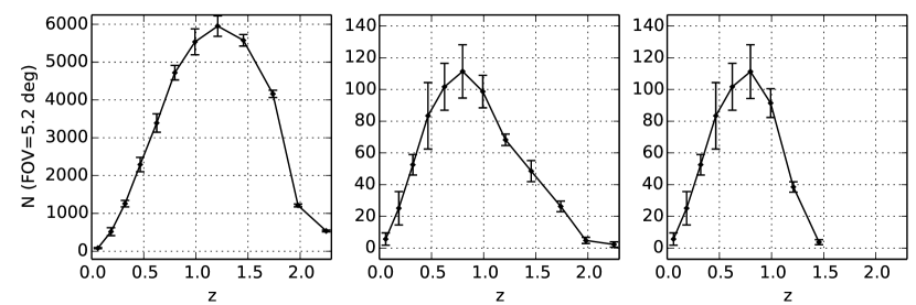
Figure 2: Halo counts as a function of redshift in the simulated field of view. Left: All FOF halos at $z<2.25$ with $N_{h}\geq 600$. Middle: All halos with FOF-derived mass $M_{\mathrm{FOF}}>10^{14}M_{\odot}\,h^{-1}$. Right: Halos with $M_{\mathrm{FOF}}>10^{14}M_{\odot}\,h^{-1}$ and $\theta_{\mathrm{vir}}>1^{\prime}$. Error bars indicate sample variance as estimated from multiple realisations of the deep field.

III.3 SPH interpolations

For each FOF identified halo, we calculate the 3D distribution of quantities like mass, temperature, etc. on a grid using a generic SPH interpolation algorithm (Gingold & Monaghan 1977; Lucy 1977) referred to as the “scatter” scheme in Hernquist & Katz (1989). Thus the local density estimate at location $\mathbf{x}$ due to a set of particles can be obtained from

$$\rho(\mathbf{x})=\sum_{i}m_{i}W(|\mathbf{x}-\mathbf{x_{i}}|,h_{i})$$ (2)

where $m_{i}$ is the mass of $i$’th SPH particle, situated at $\mathbf{x}_{i}$. $W(|\mathbf{x}-\mathbf{x_{i}}|,h_{i})$ is the smoothing kernel which we take to be the same as in the Gadget-2 code (eq.4 of Springel (2005)) with $W(|\mathbf{x}-\mathbf{x_{i}}|\geq h_{i},h_{i})=0$. $h_{i}$ is the local smoothing length of the $i$’th particle, and is calculated according to the criterion that each particle should have a constant number of neighbours. For interpolations within the same particle species, this is the same as using the criterion requiring a constant mass within the sphere of radius $h_{i}$ since all particles of a single species have the same mass. The latter criterion is used for all massive particles in density calculations in the SPH code Gadget-2. For our main results we use a fixed number of neighbours, $N_{\mathrm{neigh}}=33$. See the sections VI and IV.4 for a discussion of this choice for $N_{\rm neigh}$. Given a density estimate, the mass overdensity $\delta(\mathbf{x})=\frac{\rho(\mathbf{x})}{\rho_{c}(z)}$, where $\rho_{c}(z)=\frac{3H^{2}(z)}{8\pi G}$ is the critical density of the Universe at redshift $z$. The local value of any other quantity, $f(\mathbf{x})$, is given by

$$f(\mathbf{x})=\sum_{i}\frac{f_{i}}{\rho(\mathbf{x_{i}})}m_{i}W(|\mathbf{x}-\mathbf{x_{i}}|,h_{i}),$$ (3)

where the summation spans all particles, but only those with $|\mathbf{x}-\mathbf{x_{i}}|<h_{i}$ contribute.

We calculate scaling relations by reconstructing the 3D mass density distributions $\rho(\mathbf{r})$ of both dark matter and gas. The 3D distributions of temperature ($T(\mathbf{r})$), and density-weighted temperature ($T_{\rho}(\mathbf{r})$), (see eq. 6) are reconstructed using only gas particles. From these we calculate the radial profiles of density $\rho(r)$, temperature $T(r)$, density-weighted temperature $T_{\rho}(r)$, and baryon gas-mass fraction $f_{\mathrm{gas}}(r)$, and hence the scaling relations.

We process the TSZE signal on a halo-by-halo basis for reasons of efficiency. High spatial resolution is required to resolve intra-cluster structure, but large cosmological volumes are required to develop sample statistics. The combination is not possible on a single grid. In consequence we create a high-density grid only around the locations that will generate a significant TSZE signal. Cool particles and low-density regions will not contribute significantly and they are neglected in the analysis. The simple creation of TSZE maps could be done by processing each SPH particle independently, as is often done in simulations. However, our present approach allows us to measuring scaling relations and assessing the effects of TSZE flux boosting due to line-of-sight (LOS) overlap of halos.

III.4 Thermal Sunyaev-Zel’dovich effect

The thermal Sunyaev-Zel’dovich effect (TSZE) in galaxy clusters alters the CMB specific intensity towards a cluster as compared to a reference direction. This effectively is seen as a frequency dependent black-body thermodynamic temperature variation of amplitude

$$\delta T\equiv\Delta T/T_{\mathrm{CMB}}=f_{\nu}y,$$ (4)

where $y$ is the Comptonisation parameter and $f_{\nu}$ encodes the spectrum of the effect. In the non-relativistic limit, and with the standard redistribution function, $f_{\nu}=x\frac{e^{x}+1}{e^{x}-1}-4$, where $x=\frac{h\nu}{k_{B}T_{\mathrm{CMB}}}$, and $h$ and $k_{B}$ are the Planck and the Boltzmann constants respectively. The Compton $y$-parameter is proportional to the LOS integral of the product of the electron number density, $n_{e}$, and electron temperature, $T_{e}$,

$$y=\sigma_{0}\int n_{e}\frac{k_{B}T_{e}}{m_{e}c^{2}}\operatorname{d}\!{l},$$ (5)

where the integral is in physical distance. Following the notation of Refregier et al. (2000) this formula can also be expressed as the integral over comoving distance via $\operatorname{d}\!{l}=ad\chi=d\chi/(1+z)$, and by introducing the number of electrons per proton $\mu_{e}^{-1}=n_{e}/(\rho/m_{p})$, where $\rho$ is the gas mass density, and $m_{p}$ is the mass of the proton, the integral can be converted to

$$y=y_{0}\int T_{\rho}(1+z)^{2}\operatorname{d}\!{\chi},$$ (6)

where $T_{\rho}\equiv T\frac{\rho}{\bar{\rho}}$ is the density weighted temperature and $\bar{\rho}=\rho_{b}=\rho_{b0}(1+z)^{3}=\rho_{c0}\Omega_{b0}(1+z)^{3}$ is the average baryon mass density at redshift $z$. The constant

$$y_{0}=\frac{\sigma_{T}\rho_{c0}\Omega_{b0}k_{B}}{\mu_{e}m_{p}m_{e}c^{2}}\approx 7.76\cdot 10^{-17}\,[\mathrm{K}^{-1}\,\mathrm{Mpc}^{-1}]$$ (7)

for the assumed cosmology, where $\sigma_{T}$ is the Thomson scattering cross-section, $m_{e}$ and $m_{p}$ are the electron and proton masses respectively, and $c$ is the vacuum speed of light. We assume a standard chemical composition, compatible with Big-Bang nucleosynthesis (helium mass fraction $Y_{p}=0.24$) in which case $\mu_{e}=1.136$. We calculate the SPH gas particle temperatures as

$$T_{e}(u)=\frac{m_{p}}{k_{B}}\mu(Y_{p})(\gamma-1)u,$$ (8)

where $u$ is the internal energy per unit mass associated with a given SPH particle and $\gamma=5/3$ is the ratio of specific heats for a monatomic gas. The mean molecular weight $\mu=\frac{4}{8X_{p}+3Y_{p}}\approx 0.588$ for a fully-ionised hydrogen/helium mixture, which is the case for the intra-cluster medium. $X_{p}=1-Y_{p}$ is the mass fraction of hydrogen, and we neglect the minor contribution from heavier elements. Using eq. 4 and first-order expansion of the black body specific intensity

$$B_{\nu,\mathrm{CMB}}(x)=\frac{2\nu^{2}}{c^{2}}\frac{h\nu}{e^{x}-1},$$ (9)

about the black body temperature, it is easy to show that the TSZE-induced radiance variation $\Delta I=I_{\nu}(T)-I_{\nu}(T_{\mathrm{CMB}})$ for a cluster is

$$\Delta I=\frac{2(k_{B}T_{\mathrm{CMB}})^{3}}{(hc)^{2}}\frac{x^{4}e^{x}}{(e^{x}-1)^{2}}f(x)y=I_{0}g(x)f(x)y$$ (10)

where $g(x)=x^{4}e^{x}/(e^{x}-1)^{2}$ and $I_{0}=\frac{2(k_{B}T_{\mathrm{CMB}})^{3}}{(hc)^{2}}$. Then the TSZE flux density per beam can be calculated as

$$\Delta S_{\mathrm{TSZ}}(\nu,P_{b})=\int\Delta I_{\nu}(\mathbf{\hat{n}})P_{b}(\mathbf{\hat{n}})\operatorname{d}\!{\Omega}$$ (11)

where $P_{b}(\mathbf{\hat{n}})$ is the instrumental beam profile.

Following Nagai et al. (2007), we also define the solid-angle integrated Compton $y$-parameter as:

$$Y^{\mathrm{INT}}=d_{A}^{2}(z)\int y\operatorname{d}\!{\Omega}$$ (12)

to test the compatibility of our simulational procedures with similar simulations via the $M$-$Y$ scaling relations.

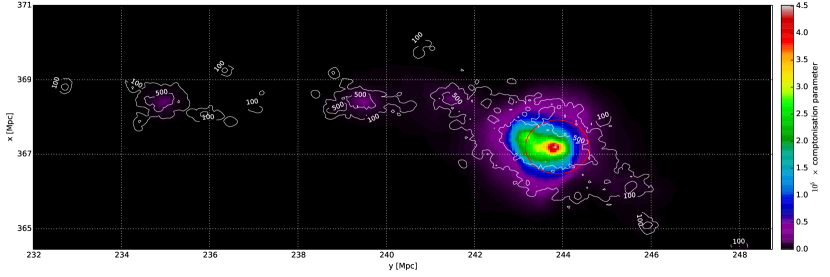
Figure 3: One of the most massive simulated galaxy cluster systems found by FOF at $z\approx 0.624$. The colour scale indicates the value of the Compton $y$-parameter, while the contours indicate the iso-overdensity regions for $\delta=\{100,500\}$ in the projected, line-of-sight–maximised mass overdensity distribution. The red circle marks a projected sphere of radius $r_{500}$ centred at the minimum of the gravitational potential of the whole system. The total halo mass is $M_{\mathrm{FOF,tot}}\approx 7.4\times 10^{14}\mathrm{M}_{\odot}h^{-1}$, and this halo is resolved with over $5.4\times 10^{4}$ dark matter and gas particles.

In figure 3 we plot an example of a system of halos. This example indicates how the FOF algorithm connects different halos into a single system if they form a filamentary structure. It is likely that other methods (such as those based on spherical overdensity) or a hierarchical approach would identify this system as a set of nested individual systems, however it is not obvious that processing the individual halos separately for calculation of (e.g.) density profiles would provide a better $r_{\delta}$ estimate because this could represent a gravitationally bounded system during a merger event, when the (over)density profiles should include the substructures. The presence of sub-halos also undermines the usefulness of radial profiles, at least at low overdensities, by the implicit assumption of spherical symmetry.

The reliability of temperature and density profile reconstructions from the point of the minimum of gravitational potential is illustrated by Figures 3 and 4. In these figures it is clearly seen (i) that the Compton $y$-parameter traces the cluster mass distribution, and (ii) that the location of the maximum $y$ (relative to which the flux density is calculated) coincides well with the minimum of the gravitational potential (the centre of the red circle). The radius of the red circle, $r_{500}$, is calculated within the spherical region enclosing the mass that yields overdensity $\delta=500$. It is evident that this $r_{500}$ roughly coincides with the contour tracing the same overdensity value.

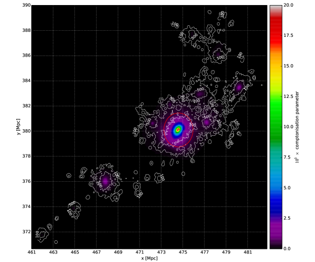
Figure 4: Same as figure 3, but for a halo of mass $M_{\mathrm{FOF,tot}}\approx 2.5\times 10^{15}\mathrm{M}_{\odot}h^{-1}$ which is resolved with more than $1.8\times 10^{5}$ dark matter and gas particles, and is evolved up to $z\approx 0.06$. As indicated by the colour scale, the TSZE signal is more than four times larger than in figure 3. However the chance of finding halos such as this in small-field surveys is low, due to the small survey volume and the low number density of halos of such high mass (figure 7).

In dynamic situations, such as those shown in figures 3 and 4, the kinematic SZ effect (kSZE) increases towards regions of the infalling gas lying close to the line of sight. While the kSZE is much smaller than the TSZE, it can dominate in regions of cold and fast-moving gas. Because the kSZE tends to be averaged out by superpositions along the line of sight, since the sign of the kSZE reverses with the sign of gas velocity, in the current paper we neglect kSZE contributions to the change of CMB intensity.

III.5 CMB simulations

We generate the CMB background fluctuation field starting from a random realisation of a lensed CMB power spectrum, generated with CAMB (Lewis et al. 2000). A random Gaussian realisation of the $a_{\ell m}$ coefficients in spherical harmonic space up to $\ell_{\rm{max}}=4096$ was then made, and a spherical harmonic transformation then converted this to the sky map of CMB temperature fluctuations. All cosmological parameters are as in section III. For the selected field we project CMB fluctuations from the Healpix grid (Górski et al. 2005) to a tangent plane, and interpolate (using the SPH interpolation algorithm) onto the regular Cartesian grid coincides our map. The Healpix map used for interpolation is significantly larger than the final map to allow for interpolation to the edge of the required area. Using this approach we can generate maps of arbitrary resolution without producing spurious signals, since the CMB fluctuations are sufficiently smooth and well resolved by the initial Healpix grid, which has resolution parameter $n_{s}=2048$. The instrumental beam is introduced (when needed) by convolving with the beam transfer function over the full sky in spherical harmonic space, rather than by FFT (Fast Fourier Transform) performed in the selected field, so that there are no induced aliasing effects.

In the flat field limit a set of $(\Delta_{\lambda},\Delta_{b})$ offsets in coordinate directions $(\lambda,b)$ approximate a spherical square. While this approximation is useful for plotting two-dimensional maps of small fields, for large FOVs it necessary to work on a grid defined over the full celestial sphere (such as Healpix). We choose the $b$ coordinate to coincide with galactic latitude, but $\lambda$ is taken to be a great-circle coordinate orthogonal to $b$, so its orientation depends on direction.

We prefix tangent plane coordinates by “$\Delta$” in order to indicate that these are the offsets with respect to the chosen field centre.

III.6 Field of view projections

The TSZE due to a given halo is calculated using its properties at the epoch closest, in terms of the redshift, to the redshift inferred from the location of the halo in our light-cone construction (also referred to as a “deep field”).

The comoving coordinates of the halo in the deep field $(x_{h},y_{h},z_{h})$ are related to the coordinates in the 2D FOV $(\Delta_{\lambda}$, $\Delta_{b})$ by

$$\begin{array}[]{ccc}\Delta_{\lambda}(x_{h},z)&=&\mathrm{atan}\bigl{[}\frac{(x_{h}-L/2)/(1+z)}{d_{A}(z)}\bigr{]}\\ \\ \Delta_{b}(y_{h},z)&=&\mathrm{atan}\bigl{[}\frac{(y_{h}-L/2)/(1+z)}{d_{A}(z)}\bigr{]},\end{array}$$ (13)

where the observer is located at $(x,y,z)=(L/2,L/2,0)$, $L$ is the comoving size of the simulation box, and $d_{A}(z)$ is the angular diameter distance at redshift $z$, corresponding to the comoving distance at redshift $z_{h}$. For TSZE signal map-making we consider every halo if it at least partially overlaps with the FOV. Partial overlaps are common for halos with low $z_{h}$ and large angular sizes.

III.7 Point source simulations

III.7.1 Flux density

We simulate contributions to the integrated flux density due to unresolved extra-galactic non-thermal sources based on source counts from AT20GB, a 20-GHz southern equatorial hemisphere blind survey (Murphy et al. 2010), and the SZA (Sunyaev-Zel’dovich Array) 31-GHz blind survey of about 4.3 $\rm{deg}^{2}$ (Muchovej et al. 2010). AT20GB is complete at 78% above flux density 50 mJy. The SZA survey is complete at 98% above flux density 1.4 mJy. Although we do not directly use the 15-GHz 9C results(Waldram et al. 2003), we find that counts based on the 9C survey are consistent with those from the other two surveys within the uncertainties, when corrected for the frequency and completeness.

In the low flux-density limit we use the SZA survey, which probes the flux density range (0.7,15) mJy, and extrapolate from 15 mJy to 50 mJy, based on the best fit power-law model of the form $\operatorname{d}\!{N}/\operatorname{d}\!{S}=A(S/S_{0})^{-\gamma}$, with parameters as given in table 2. We calculate the spectral index distribution required for our extrapolation only for SZA sources fainter than 30 mJy.

In the flux density range above 50 mJy we use the AT20G survey which covers a wide area and hence is well-suited to probe the strong radio source population. Our comparison of the two surveys, at a single frequency based on our spectral model, indicates that the SZA survey predicts slightly more faint sources than AT20G.

We simulate the $\operatorname{d}\!{N}/\operatorname{d}\!{S}$ relation for the three target frequencies, 15, 22, and 30 GHz, using Monte-Carlo realisations of a skew-Gaussian–fitted probability distribution function (PDF) (eq. 15) of spectral indexes $\alpha_{8-20}$ for the AT20GB survey and $\alpha_{5-31}$ for the SZA survey respectively, where $\alpha_{\mathrm{f_{1}-f_{2}}}$ is the spectral index of a source between frequencies $f_{1}$ and $f_{2}$. Our convention for the sign of spectral index is that

$$S(\nu)=S_{0}\Bigl{(}\frac{\nu}{\nu_{0}}\Bigr{)}^{-\alpha},$$ (14)

and the flux density measurements at the reference frequencies were provided with the catalogue data.^, The fitting function for the spectral index distributions $\operatorname{d}\!{N}/\operatorname{d}\!{\alpha}$ take the form

$$\phi(\alpha,A_{\alpha},m_{\alpha},\sigma_{\alpha},S_{\alpha})=A_{\alpha}\exp\Bigl{(}-\frac{(\alpha-m_{\alpha})^{2}}{2\sigma_{\alpha}^{2}}\Bigr{)}\Bigl{(}1.0+\mathrm{erf}\bigl{(}S_{\alpha}\frac{\alpha-m_{\alpha}}{\sigma_{\alpha}\sqrt{2}}\bigr{)}\Bigr{)}$$ (15)

where $\mathrm{erf}$ is the error function.

We use the Levenberg-Marquardt (LM) algorithm (Levenberg 1944; Marquardt 1963) to find the best-fit parameter values. In order to avoid getting trapped in the local minima of the likelihood function, we use a Monte-Carlo approach to generate initial parameter guesses from within a parameter space that extends beyond the range of plausible parameter values. We impose a flat prior on each of the initial parameters values in every LM run. We fit spectral index distributions as shown in Figure 5, with parameters $(A_{\alpha},m_{\alpha},\sigma_{\alpha},S_{\alpha})$ as given in table 2.

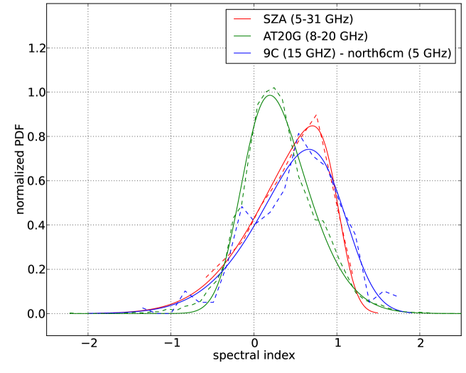
Figure 5: Spectral index distributions based on the SZA 31-GHz survey (dashed red), the AT20G survey (dashed green), and the 9C survey data cross-correlated with the North6cm survey (dashed blue), with corresponding skew-Gaussian distributions (solid lines) as in equation 15. The fitted parameters are given in table 2.

Table 2: Best-fit parameters for the skew-Gaussian distributions (equation 15) of spectral indexes for the 9C, AT20GB, and SZA radio catalogues. The last four columns give the amplitude and the tilt of the power-law $\operatorname{d}\!{N}/\operatorname{d}\!{S}$ relation (for pivot flux density $S_{0}=1\,\mathrm{mJy}$), the assumed catalogue completeness, and frequency respectively.

Catalogue name	$A_{\alpha}$	$m_{\alpha}$	$\sigma_{\alpha}$	$S_{\alpha}$	$A$ $[\mathrm{Jy}^{-1}\mathrm{sr^{-1}}]$	$\gamma$	$f_{c}$	$\nu$ $[\mathrm{GHz}]$
9C	$0.471\pm 0.058$	$1.075\pm 0.073$	$0.816\pm 0.109$	$-2.49\pm 1.04$	51.0	2.15	1.00	15.2
AT20GB	$0.641\pm 0.055$	$-0.120\pm 0.040$	$0.603\pm 0.055$	$2.26\pm 0.42$	31.0	2.15	0.78	20.0
SZA	$0.475\pm 0.070$	$1.018\pm 0.063$	$0.809\pm 0.138$	$-4.61\pm 2.83$	30.4	2.18	0.98	31.0

The fit to the AT20G survey slightly underestimates the number of sources with inverted spectra. The 9C survey suggests the presence of a population of inverted-spectrum sources at a level not present in the other two distributions. Since statistical significance of this feature is poor, we prefer to use the simple skew-Gaussian models, rather than the superposition of two spectral populations of sources, in constructing our model skies.

The differences in the estimated spectral index distributions and in differential source counts resulting from different surveys make the predictions at the target frequencies inaccurate at the level of several percent, with the degree of mismatch being a function of the flux density range of interest, the survey sensitivity, and the estimated coverage completeness.

For the assumed field size of $5.2\,\rm{deg}^{2}$ we generate 100 Monte-Carlo realisations of point source flux density distributions at the original catalogue frequencies. The flux density PDFs are probed within the range from 1 $\mu$Jy to 1 Jy. We then generate random realisations of the spectral indexes according to the spectral index PDF (eq. 15) generated for a given catalogue and create a Monte-Carlo realisation of the flux densities at the target frequency of interest using eq. 14. We then combine the realisations from the AT20GB and SZA catalogues by removing sources below 50 mJy for the AT20GB simulation and above 50 mJy for the SZA simulation.

The result is plotted in Figure 16 as a cumulative distribution, is discussed in Section V.

In order to avoid extrapolations below the measurement-probed flux densities ($S$) for simulations of point source flux density embedded in our mock maps, we only use the sources with $S>100\,\mu\mathrm{Jy}$.

While we treat all unresolved sources as sources of a constant pixel-size angular extent, a more realistic simulation could account for the fraction of the radio sources that will be resolved by the telescope beam. However, the vast majority of sources of interest for our purposes will be unresolved, and we ignore this possibility for the present.

III.7.2 Spatial correlations

Radio sources tend to cluster towards galaxy clusters (e.g. Coble et al. (2007)). We assess this for the specific case of radio sources and clusters with strong TSZ effects by cross-correlating the NVSS catalogue (Condon et al. 1998) of radio sources with the early Planck-SZ cluster candidates sample (Planck Collaboration et al. 2011).

We calculate the average cumulative number density of radio sources per unit solid angle $\rho_{N}(\theta_{\mathrm{max}})$ as a function of angular distance from the cluster centre

$$\rho_{N}(\theta_{\mathrm{max}})=\frac{1}{\pi\theta_{\mathrm{max}}^{2}N_{0}}\int_{0}^{\theta_{\mathrm{max}}}\frac{\partial N(\theta)}{\partial\theta}\operatorname{d}\!{\theta}\approx\frac{1}{\pi\theta_{\mathrm{max}}^{2}N_{0}}\sum_{i}A_{1}(\theta_{i})$$ (16)

where $A_{1}(\theta_{i})=1$ if the radio source is at angular distance $\theta_{i}<\theta_{\mathrm{max}}$ from its associated cluster’s centre and $A_{1}=0$ otherwise. The summation extends over all radio sources. $\partial N(\theta)/\partial\theta$ is the differential radio source count as a function of radial angular distance from the cross-correlated cluster centre, and the $N_{0}$ factor is taken as the total number of clusters in the sub-sample selected for a given redshift range. It therefore calibrates the relation allowing for comparison of data sub-samples of different sizes. The result is shown in the figure 6. If point sources around galaxy clusters were not clustered but rather uniformly distributed, $\rho_{N}(\theta_{\mathrm{max}})$ would be a constant function, and equal the average number density ($\langle\rho_{N,\mathrm{NVSS}}\rangle$) defined by the survey sensitivity threshold. Figure 6 clearly shows that this is not the case. For the NVSS survey $\langle\rho_{N,\mathrm{NVSS}}\rangle\approx 0.0135\,\mathrm{arcmin}^{-2}$, which is simply the total number of sources in the catalogue ($1\,810\,672$) divided by the total survey area ($2326\times 4^{2}$ $\mathrm{deg}^{2}$).

We find that the $\rho_{N}(\theta_{\mathrm{max}})$ relation is redshift dependent and exhibits somewhat stronger clustering at higher redshifts. The redshift dependence results in part from the larger angular sizes of cluster of a given mass at lower redshifts, but also from the Planck cluster selection function. A full analysis of the statistical properties of point source clustering around TSZE-detected clusters would be complicated, but for the purpose of this work, we use our result to infer that radio sources are roughly 10 times more abundant in galaxy cluster centres than in their peripheries (figure 6 right panel). The Planck-SZ sample (Planck Collaboration et al. 2014a) yields lower central clustering values by several per-cent, hence our choice may be conservative when inferring the effective SZ-cluster counts.

Thus we simulate the direction-dependent radio source density by constructing a two-dimensional probability distribution function (PDF) for a source’s appearance using the locations of CDM halos extracted from the deep field simulations. The shape of an individual PDF component due to a single halo is assumed to be a two-dimensional Gaussian with full width at half maximum defined by the halo virial diameter. Its amplitude is proportional to the halo virial mass. This is motivated by the heaviest halos being the richest in galaxies, and hence likely to contain more radio sources. If the virial quantities are not defined (due to too small overdensity) we use instead the halo total FOF extents along the directions tangential to the LOS and the total FOF masses. The location of individual PDF maximal values coincide with the directions towards the minima of the gravitational potential. We then use Monte-Carlo realisations to create a point source distribution with fluxes generated as described in section III.7.1. The resulting map is converted to units of specific intensity for the assumed angular resolution of the map and added to the simulated maps of the TSZE component.

The choice of a Gaussian shape for the correlated components of the PDF could, in principle, be replaced by the $\beta$-like profiles. The shape of a Gaussian differs from that of a $\beta$ profile, in particularly by showing a faster decrease at large angular distances from the halo centre. However, since the background source density is about 10% of the peak source density, we expect the shape assumption to have little effect on generic results from our simulations. Furthermore, the observational data (figure 6) do not give strong evidence for either shape, at present.

In addition to the correlated component of radio sources, we also insert a uniformly-distributed source population in the field adding a constant density to the PDF. This simulates high-redshift sources outside the redshift range of the simulation, ignoring the (usually weak) effects of gravitational lensing. The constant source density used depends on the survey flux density threshold, which for the NVSS is about $\sim 2.5\,\mathrm{mJy}$ – the flux density corresponding to the weakest detected sources (Condon et al. 1998). Although this constraint is similar to independent estimates reported in Coble et al. (2007) one would obtain a slightly different radio source overdensity values if the clusters sample was cross-correlated with a survey of a different sensitivity.

We neglect the contributions from the thermal sources as they are not dominant in the considered frequency range.

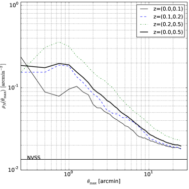
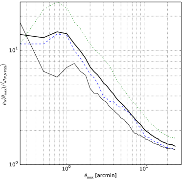
Figure 6: (left) The average NVSS survey point source number density per unit solid angle around the centroids of Planck TSZE-selected cluster candidates as a function of the angular distance from the suspected cluster centres. The solid-thin (black), dashed (blue), dot-dashed (green) and solid-thick (black) lines represent the densities for sub-samples selected according to the redshift range given in the plot legend. The horizontal line indicates the average number density of point sources for the NVSS survey. (right) The relative overdensity of point sources for the same redshift sub-samples with respect to the NVSS survey.

IV Comparison to other simulations, observations and theoretical predictions

In the following sections we test our simulations of structure formation by comparing selected scaling relations with those from other simulations and with observations provided by the Chandra and the XMM-Newton satellites. We also test the consistency of the extracted mass functions with the theoretical predictions of the Press-Schechter theory and fitting functions fixed by other numerical simulations.

IV.1 Halo mass function

In figure 7 we plot the mass function $\operatorname{d}\!{n}/\operatorname{d}\!{M}$ of the FOF halos identified in our deep-field simulations, sliced at the hypersurface of the present. We also show the Press-Schechter (PS) mass function (Press & Schechter 1974) calculated with the same cosmological parameters

$$\frac{\operatorname{d}\!{n}_{\mathrm{PS}}}{\operatorname{d}\!{M}}=\sqrt{\frac{2}{\pi}}\frac{\rho_{m}}{M}\frac{\delta_{c}}{\sigma(M)}\frac{\operatorname{d}\!{\ln}\sigma^{-1}(M)}{\operatorname{d}\!{M}}\exp\Bigl{(}-\frac{\delta_{c}^{2}}{2\sigma^{2}(M)}\Bigr{)}$$ (17)

where $\sigma(M)=\sigma(M(R))$ with $M(R)=\frac{4}{3}\pi R^{3}\rho_{m}$ and

$$\sigma^{2}(R)=\int P_{g}(k)W^{2}(kR)\frac{\operatorname{d}\!{k}}{k},$$ (18)

is the variance of the matter density fluctuations smoothed at scales $R$.

$$P_{g}(k)=\frac{4}{25}f^{2}(\Omega_{m},\Omega_{\Lambda})\Bigl{(}\frac{k}{a_{0}H_{0}}\Bigr{)}^{4}T^{2}(k)\mathcal{P}_{\mathcal{R}}(k)$$ (19)

is the power spectrum of the mass density distribution (in units where $c=1$). In equation 19 $\mathcal{P}_{\mathcal{R}}(k)=\Delta_{\mathcal{R}}^{2}(k/k_{0})^{n_{s}-1}$ is the power spectrum of primordial curvature perturbations with pivot scale $k_{0}=0.002\,\mathrm{Mpc^{-1}}$, $T(k)$ is the matter transfer function, and $f(\Omega_{\Lambda},\Omega_{m})\equiv\frac{g(\Omega_{\Lambda},\Omega_{m})}{\Omega_{m}}$ is the $\Lambda$CDM linear perturbation growth factor relative to the Einstein-de-Sitter case. The $g(\Omega_{\Lambda},\Omega_{m})$ quantity is model dependent, and for the flat $\Lambda$CDM model is given by the fitting formula as in eq. 29 of Carroll et al. (1992). In that formula the variable names are different so it’s not a direct reference. The kernel function $W(kR)$ is chosen to be the Fourier transform of the top-hat function and its exact form depends on the assumed Fourier transform convention. The quantity $\delta_{c}=1.69$ is the present linear-theory overdensity required for a uniform spherical region to collapse into a singularity and it has a weak dependence on cosmological parameters (Eke et al. 1996). We use the CAMB software to obtain a high resolution $\Lambda$CDM matter transfer function, tabulated up to $k\eta_{\mathrm{max}}=1.5\times 10^{5}$ (where $\eta_{\mathrm{max}}$ is the comoving scale of particle horizon). This is required for accurate predictions for the lowest-mass halos.

We also compare our results with the Tinker mass function (Tinker et al. 2008) at redshift $z=0$

$$\frac{\operatorname{d}\!{n}}{\operatorname{d}\!{M}}=f(\sigma(M))\frac{\rho_{m}}{M}\frac{\operatorname{d}\!{\ln}\sigma^{-1}(M)}{\operatorname{d}\!{M}},$$ (20)

for the overdensities $\delta=\{100,200\}$ which should enclose the range statistically probed by the FOF algorithm with linking length parameter $b=0.2$. The Tinker mass function is parametrised by

$$f(\sigma(M))=A\Bigl{[}\Bigl{(}\frac{\sigma(M)}{b}\Bigr{)}^{-a}+1\Bigr{]}\exp\bigl{[}-\frac{c}{\sigma^{2}(M)}\bigr{]},$$ (21)

where the four parameters $(A,a,b,c)$ are linearly interpolated (and extrapolated for the case of $\delta=100$) based on the values tabulated in table 2 of Tinker et al. (2008).

Figure 7 shows that there is a good consistency between the recovered FOF mass function and the theoretical expressions at $z\approx 0$, confirming that our numerical calculations are robust, and supporting the validity of the halo abundances in our light-cone realisations. Apart from the known underestimate of the abundance of the heaviest halos made by the Press-Schechter mass function, the extracted mass function seems to overestimate the abundance of heavy halos with respect to the Tinker mass function, and slightly underestimate it (by a factor $\approx 1.02$ with respect to the Tinker prediction at $\delta=200$) for the lightest halos, which have $N_{h}$ only slightly above the minimum of $600$ (section III.2).

This effect could be explained by the tendency of the FOF algorithm to connect multiple light halos into single, heavier systems (as depicted in figure 3 and figure 4). For the same reason, and because of the limited mass resolution of our simulations, for low-mass halos the reconstructed mass function slightly deviates from the Tinker mass function prediction. Details of the MF redshift evolution do not have impact on most of the presented results (but see section V.3.6 where an order-of-magnitude estimates are obtained by neglecting the MF redshift evolution up to redshift $z=1$).

We find that the creation of the low-mass halos is sensitive to the settings of the softening length in the gravity computations. Too large a softening length may significantly suppress light halo abundance and underestimate baryon temperature. Decreasing the softening length significantly increases the computational time. We experimented with various softening lengths to check that the value of $\sigma_{8}$ calculated in the simulations is consistent with the input, linearly-predicted, value. We found that a softening length of 15 kpc/$h$ provides reasonably-converged $\sigma_{8}$ values for our mass resolution with acceptable execution times. The overall consistency between our mass function and that from the Tinker mass function assures us that our halo abundances are realistic.

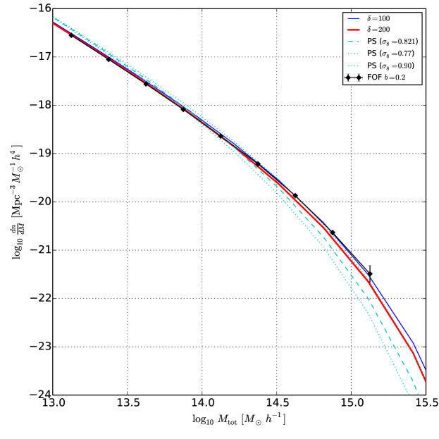
Figure 7: Average halo mass function resulting from several realisations of the simulation box comoving volume (black diamonds), compared with the Press-Schechter (dashed, cyan) and Tinker (solid) mass functions for a LCDM model. Results are shown for $\delta=100$ (blue,thin) and for $\delta=200$ (red,thick) overdensity thresholds. The error bars correspond to $\pm 1\sigma$ from sample variance in our simulations. The dotted (cyan) lines are the PS predictions that show the impact of a different $\sigma_{8}$ normalisations.

IV.2 The M-$\sigma_{v}$ scaling relation

In order to further test the initial conditions and the compatibility of the assumed cosmology with observations we compare the velocity dispersions measured in the simulated halos with the LOS velocity dispersions measured in Abell clusters. On the simulation side as a measure of the velocity dispersion we choose the square root of the mean dark matter halo coordinate-velocity variance: $(\langle\sigma_{v_{i},\mathrm{vir,DM}}^{2}\rangle_{i})^{1/2}$, calculated within spheres of virial radius We plot these estimates against the total viral mass of halos $M_{\mathrm{vir}}$ to construct the $M-\sigma_{v}$ scaling relation, which for the case of virialised clusters should follow

$$\sigma_{v}(M_{\delta})=\sigma_{15}\Bigl{(}\frac{M_{\delta}}{10^{15}M_{\odot}/h}\Bigr{)}^{\alpha_{v}}[\mathrm{km/s}],$$ (22)

with $\alpha_{v}=1/3$, where $\sigma_{15}$ is the calibration of the relation at the mass scales of $10^{15}M_{\odot}/h$. In figure 8 we plot the cluster masses and line-of-sight velocity dispersions of our simulated halos together with the reconstructed cluster masses and velocity dispersions from Łokas et al. (2006). This compilation provides the best-fit masses of six nearby ($z<0.06$) galaxy clusters within their virial radii, and were found by fitting solutions of Jeans equation to the reconstructed cluster velocity variance and velocity kurtosis profiles, assuming the validity of their NFW density profiles to the virial radii. The cluster velocity dispersion profiles, as probed by large galaxies, were derived from the NASA/IPAC Extragalactic Database (NED) with a selection including a test to reject likely merging systems, as described by Łokas et al. (2006). We also plot the reconstructed $M-\sigma_{v}$ scaling relation from a projected phase-space analysis for the sample of nearby Abell clusters reported in Wojtak & Łokas (2010), where different methods of mass estimation are discussed. We ignore the small difference in the virial overdensity definition between the value assumed for this analysis and that of Łokas et al. (2006).

The reconstructed velocity dispersion follows the virialised cluster scaling relation well, and the simulated clusters have realistic velocity dispersions, with no significant mass resolution effect.

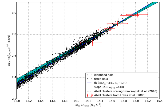
Figure 8: The M-$\sigma_{v}$ scaling relation for the sample of simulated halos (black dots) is compared against the measurements of the line-of-sight velocity dark matter dispersion in Abell clusters as derived in Łokas et al. (2006) (red diamonds). The solid line is the fitted power law scaling relation, equation 22, and the dashed line is the fitted scaling relation for power-law slope $\alpha_{v}=1/3$. The fitting is done only for halos indicated by large dots, with $M_{\mathrm{vir,tot}}>10^{14}\ M_{\odot}h^{-1}$. For clarity, we plot only 10% of the halos with $M_{\mathrm{vir}}<10^{14}\ M_{\odot}h^{-1}$. The dotted line with shaded area is the scaling relation reported in Wojtak & Łokas (2010) using a larger sample of Abell clusters.

IV.3 The M-T scaling relation

In this section we test our simulations against the mass-temperature scaling relation.

Our simulation framework relies on the adiabatic gas approximation (AD) and the resulting temperature profiles therefore deviate from those extracted from simulations that include radiative cooling, star formation, and AGN or supernova feedback (hereafter CSF). Such processes play an important role in explaining cool-core clusters, and may be required to fine-tune simulations to observational data, especially in cluster central regions. In the central parts of clusters the strong radiative cooling due to thermal processes dominates over the heating from processes associated with star formation, while in cluster outskirts the net effect results in an increase of the ICM temperature (Nagai et al. 2007). This difference alters ICM density profiles to some extent, and should affect the profiles of cluster X-ray emission and Compton $y$-parameter. The difference between the AD and CSF cases is estimated to be a few tens of per-cent. This is seen in figure 9. In our AD simulations we find gas temperatures systematically lower than as reported from CSF simulations, by a factor $\sim 1.3$ at $\delta=500$.

As in section IV.2, we examine the $M$-$T$ scaling relation for our simulated sample of heavy halos and fit a scaling relation to those with $M_{500,\mathrm{tot}}>10^{14}M_{\odot}/h$. A low-mass cut-off is required to avoid the biases resulting from our limited mass resolution. Mass resolution effects also become increasingly important at large $\delta$, and lead to artificial deviations from self-similar scaling. For the adiabatic case the cluster gas temperature is expected to scale self-similarly with the cluster mass (Kaiser 1986)

$$T(M_{\delta})=T_{15}\Bigl{(}\frac{M_{\delta}E(z)}{10^{15}M_{\odot}/h}\Bigr{)}^{\alpha_{T}}[\mathrm{keV}],$$ (23)

where $\alpha_{T}=2/3$, $T_{15}$ is the scale temperature at mass $10^{15}M_{\odot}/h$, and $E(z)=\sqrt{\Omega_{m0}(1+z)^{3}+\Omega_{\Lambda 0}}$.

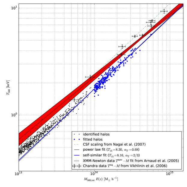
Figure 9: Halo-mass–temperature scaling relation for halos identified in the lowest-redshift simulation ($z\sim 0.06$) for $\delta=500$. Small (black) dots indicate the FOF identified halos and large (blue) dots indicate the halos used for fitting the scaling relation defined in equation 23. We discard halos with masses $M_{500}<10^{14}M_{\odot}h^{-1}$ and outliers identified as points deviating from the initial whole-sample power-law fit 10%. For clarity, we plot only every tenth halo with $M<10^{14}M_{\odot}h^{-1}$. The solid lines indicate the power law two parameter fit (thick,blue) and the self similar fit (thin,black) to the filtered data. The scaling relation of Nagai et al. (2007), from high mass-resolution simulations that include radiative cooling and star formation effects, and assuming a self-similar slope, is shown by the dash-dotted line. Data for the scaling relation for gas-mass weighted temperature are taken from Vikhlinin et al. (2006) (black diamonds). The best-fit scaling relation using spectroscopic temperature from Arnaud et al. (2005) is shown as the dotted line with the 1-$\sigma$ uncertainty band (shaded red) under assumption of zero covariance between amplitude and power-law index. The tens of percent discrepancy between the adiabatic simulations and the observations is known to be the result of gas physics not included in our simulations.

We observe that the scaling relation (as probed by the simulated halos) clearly follows the self-similar prediction for high-mass clusters, but apparently underestimates the cluster temperature at $\delta=500$. The low-mass tail deviates from self-similar scaling. We verified that this is due to the limited mass resolution in our $2\times 512^{3}$ particles simulation, and is the main reason why we neglect lighter halos in fitting the scaling relations. In order to exclude outliers we perform the fitting in two stages. First we fit a straight line in the space of logarithms of masses and temperatures, calculate relative residuals, and exclude halos that deviate by more than 10%. Then we perform the second fit on such pre-filtered data. Halos ignored in the fitting process are marked with small dots in figure 9. In the particular case of the scaling relation calculated from the simulation presented in the figure 9 there are no outliers within the fitted mass range. In that figure we also provide a power-law fitting function parameters for the cases of (i) fixed slope (according to the self-similar case) and (ii) with fitted slope.

In our 3-D gas temperature reconstructions (section III.2) it is assumed that the degree by which our adiabatic approximation simulations deviate from the actual temperature distributions in the forming clusters is similar throughout the whole range of the considered redshifts (section III.1).

IV.4 The M-Y scaling relation

As a final consistency test we compare the M-Y scaling relation from our simulations with that from a similar, but higher mass-resolution, adiabatic simulation performed in Nagai (2006).

Figure 10 shows over 2000 of the most massive halos found in one of the simulations evolved up to the redshift of $z=0.06$. The $M-Y^{\mathrm{INT}}$ relation for self-similar evolution is given by

$$Y^{\mathrm{INT}}(M_{\delta})=\Bigl{(}\frac{Y_{14}}{10^{6}}\Bigr{)}\Bigl{(}\frac{M_{\delta}}{10^{14}M_{\odot}/h}\Bigr{)}^{\alpha_{Y}}E(z)^{2/3}[\mathrm{Mpc^{2}}],$$ (24)

with $\alpha_{Y}=5/3$ and where $Y_{14}$ is scale Comptonisation parameter at mass scale $10^{14}M_{\odot}/h$. This relation follows from equations 23 and  12. As before, we fit the scaling relation using the LM algorithm supported Monte-Carlo selection of initial parameters for individual LM minimisations. The data filtering and fitting strategy is as described in section IV.3.

We find that the $M-Y$ scaling relation is consistent with the results from the AD simulations of Nagai (2006) to within a factor of order unity for low $\delta$ values. The $Y_{14}$ scaling, however, depends on a number of factors, particularly on the choice of the number of neighbours used in the smoothing kernel for the SPH interpolations and density calculations. We find that 20% changes in $Y_{14}$ occur as we change the number of neighbours from 5 to 66, with larger values of $Y_{14}$ arising from a larger neighbour count. Even with our highest mass resolution ($N_{\mathrm{tot}}=2\times 256^{3}$ and $L=128$ Mpc) we find that the amplitude of the scaling relation for $\delta=500$ is larger by a factor of $\sim 1.1$ for $N_{\mathrm{neigh}}=15$ than in Nagai (2006). For $N_{\mathrm{neigh}}=33$ (used for figure 10) the calibration is larger by a factor of $\sim 1.40$ than the value $Y_{14}^{\mathrm{AD}}(\delta=500)=4.99$, and by $\sim 2.1$ from the value $Y_{14}^{\mathrm{CSF}}(\delta=500)=3.29$), from Nagai (2006). However, the scaling relation is much more similar at lower overdensity thresholds, $\delta=\{200,\mathrm{vir}\}$. In the case of $\delta=\delta_{\mathrm{vir}}$, the scaling calibration is larger only by factors $\sim 1.1$ and $\sim 1.6$ for the AD and CSF cases of Nagai (2006).

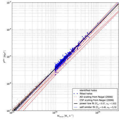
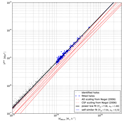
Figure 10: Halo-mass–integrated Comptonisation-parameter scaling relation for halos identified in the lowest redshift simulation ($z\sim 0.06$) for the virial (left) and $\delta=500$ (right) mass definitions. The solid lines indicate power law two-parameter fits (thick) and self-similar fits (thin) to halos with outliers removed and with total estimated FOF masses $>10^{14}\mathrm{M_{\odot}\,h^{-1}}$. For clarity, we plot only every tenth halo with mass $<10^{14}\mathrm{M_{\odot}\,h^{-1}}$. We also show the scaling relations of Nagai (2006) from high-resolution adiabatic simulations (dashed) and simulations that include radiative cooling and star formation (dash-dotted).

Mass resolution also has an important impact on the value of $Y_{14}$. As the mass resolution is improved, the amplitude of the scaling relation approaches that of the AD simulation of Nagai (2006). A 64-fold mass resolution increase, from $N_{\mathrm{tot}}=2\times 256^{3}$ and $L=512$ Mpc to $N_{\mathrm{tot}}=2\times 512^{3}$ and $L=512$ Mpc to $N_{\mathrm{tot}}=2\times 256^{3}$ and $L=128$ Mpc induces changes of order 20% in the value of $Y_{14}$.

This parameter is also affected by the choice of redshift used to generate the initial conditions. The reason probably stems from the challenge of preserving high numerical accuracy during time evolution of structure formation. This is more difficult as perturbations are followed through a broader range of density contrast (i.e., from earlier epochs).

We experimented with different numbers of neighbours at fixed mass resolution to optimise the interpolation for TSZ signals. For each SPH particle that comprises a part of a halo we investigated how precisely we could perform interpolations, weighted according to the density-weighted temperature, at grid cell centres. We used the density-weighted temperature to ensure that the interpolation error is dominated by regions that contribute most to the SZ signal and not by the cluster peripheries, where the density weighted temperature is small. We found that the relative interpolation accuracy is or order 1% as a function of number of neighbours, and that the values of $Y_{14}$ change by less than 1% as the grid resolution is improved from 50 to 25 kpc.

In figure 10 (right), we find that at overdensity $\delta=500$ there is a small departure from self-similarity at low mass, because of the limited mass resolution. The effect becomes worse for simulations with worse mass resolution, and is more noticeable at larger $\delta$, as expected.

The net effect of ignoring cooling and star formation in our simulations is an overestimation of the TSZE signal. This may result in our simulations overestimating the number of objects that would be detected for a given flux density threshold, although the amplitude of the difference between AD and CSF simulations is also a function of redshift. Thus our estimates of the number of TSZE detections may be high by a modest factor ($<2$).

V Results

We now describe the main results from this study. We split these into four categories: (i) mock maps; (ii) survey sensitivity limits; (iii) predictions for TSZE blind surveys; and (iv) predictions for blind radio-source surveys.

V.1 Mock maps

It is crucial to know the properties of the signals sought before designing the software that will extract astrophysical signals from noisy and incomplete radio-survey data. Therefore, one of the basic results of this work is a set of high-resolution maps ($10^{4}\times 10^{4}$ pixels at about 1.9 arcsec/pixel) that include contributions from CMB fluctuations, cluster TSZEs, and point sources. Sample simulated CMB and TSZE fields contributing to the frequency maps of a deep field are shown in figure 11. The top row shows the simulated CMB field with and without the CMB dipole, which takes the form $T_{d}(\mathbf{\hat{n}})=A\cos(\mathbf{\hat{d}}\cdot\mathbf{\hat{n}})$ with $A=3.346$ mK, and $\mathbf{\hat{d}}=$$(l^{\circ},b^{\circ})=(264.26,48.22)$ (Bennett et al. 2003). The significant difference between these two panels arises from the gradient in intensity across the field caused by the dipole, and the choice of field direction — $(l^{\circ},b^{\circ})=(135,40)$, chosen to lie at high galactic latitude and declination, to ensure year-round visibility and high elevation from the vicinity of Toruń.

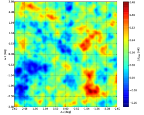
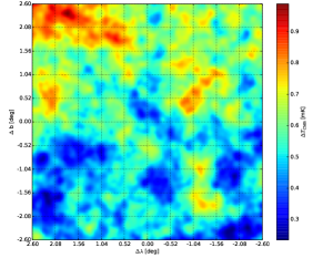
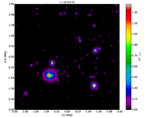
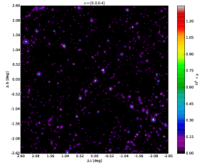
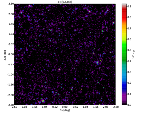
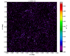
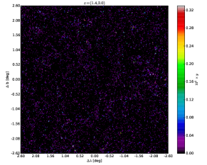
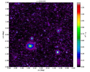
Figure 11: Simulated deep field maps, rebinned for display. Top row: CMB fluctuations without (left) and with (right) the dipole component for field centre $(l^{\circ},b^{\circ})=(135,40)$. The axes are $\pm 2.6^{\circ}$ about the field centroid, in Galactic coordinates. Second to fourth rows: simulated realisation of the TSZE signal from different redshift ranges, with the colour map scaled to emphasise the lowest 25% of the signal, with stronger signals saturated in the white. The maximum Compton $y$-parameter value in this realisation is $y\approx 5.9\times 10^{-5}$. The pixel scale, of $\sim 1.9$ arcsec is well below the FWHM of the telescope beams (table 1). The high-resolution simulation has been rebinned for display preserving the maximum $y$ per bin, rather than the bin average, in order to display the thermal energy content per cluster in each redshift range.

In a small survey it is unlikely that an extremely large TSZE, from a very massive cluster, will be found. Using the eleven stacked simulations we generated seven TSZE maps for each of the three frequencies of interest (table 1) by random permutations of the simulation box order, particle shifts, and coordinate transformations (Section III.1). The example shown in figure 11 is typical of the set, and shows the typical maximum TSZE that should be expected in a blind survey of this size, $y\lesssim 1.0\times 10^{-4}$.

Figure 12 (top row) shows the combined CMB and TSZE signals. TSZEs are seen in these images because they typically appear on small angular scales, where the CMB fluctuations tend to be weak. The RT32/OCRA-f and RTH/15 GHz beam sizes are much smaller than the angular scale scale of strong CMB background fluctuations (figure 12 right panel). An example point source realisation generated for this particular deep field is shown in the second row of the figure: the flux densities of simulated sources span more than three orders of magnitude. The spatial correlations due to point source clustering around heavy halos is evident (see the lower-right panel), even though we show only sources stronger than 0.5 mJy.

The number of galaxy clusters that can be detected in a blind survey depends on two main factors. The first is the angular size of the telescope beam: the presence of clusters with smaller scales will tend to be suppressed by the noise. This translates into a high-redshift cut-off in the survey. The same effect is intrinsically present in the cluster counts: cluster evolution means that at high redshifts clusters are less evolved, smaller, less massive, and provide weaker TSZE signals. The second factor is the survey area, and this is limited by the total integration time, receiver noise, and the size of the radio camera. Given the high-redshift cut-off from angular resolution effects, the number of detected clusters can be increased by increasing the survey area. This will pick up more low-redshift clusters, which are more massive, well resolved by the beam, and yield larger total TSZE flux densities. Larger telescopes provide better sensitivity, but in smaller beams, and so can take more time to cover the same sky area as smaller telescopes. It is for this reason that large radio cameras are highly effective, and even necessary. Larger telescopes could also use lower frequencies, and hence produce larger beams, usually with lower atmospheric noise. However, using a lower frequency comes at the cost of decreasing the TSZE intensity.

For example, a change of observation frequency from 30 GHz to 15 GHz and a dish size from 32 meters to 100 meters results nearly in 10-fold decrease in TSZE flux density, where a factor of $\frac{\theta_{b}(15\mathrm{GHz})}{\theta_{b}(30\mathrm{GHz})}\approx 1.56^{2}\approx 2.4$ is due to the beam solid angle decrease (even though the observation frequency decreased) and a factor of $\frac{f(30\mathrm{GHz})g(30\mathrm{GHz})}{f(15\mathrm{GHz})g(15\mathrm{GHz})}\approx 3.86$ is due to TSZE intensity change. This is clearly seen in the figure 14 where the TSZE flux density in RTH case is statistically about an order of magnitude smaller than in the case of the 32-metre telescope. However, in case of a small-dish survey the effective number of detected TSZE clusters is strongly limited by point source confusion. This is quantified in Figure 13 and the following sections. In the figure the effect of beamwidth change within the same frequency is clearly seen: the ratio of RTH to RT32 beam solid angles (Table 1) at 30 GHz is $\sim 10$ which directly translates onto the integrated flux density distributions.

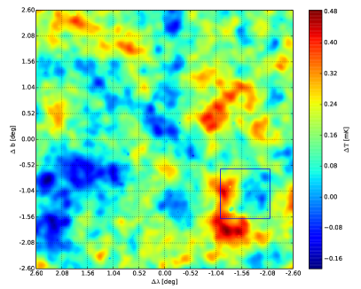
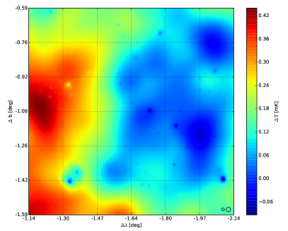
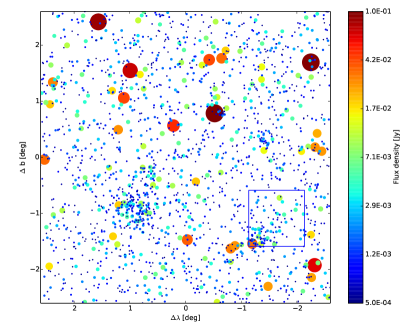
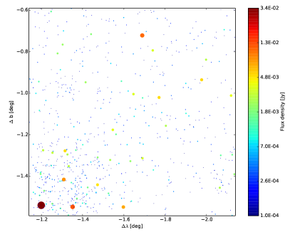
Figure 12: Simulated deep field maps, rebinned for display. Upper row: a realisation of CMB fluctuations and the 30-GHz TSZE over a $5.2^{\circ}\times 5.2^{\circ}$ field (left), with a zoom view of the $1^{\circ}\times 1^{\circ}$ region marked by a square (right). In the right-hand panel the large and small circles indicate the FWHM beam-sizes of the 30-GHz OCRA-f receiver on the 32-metre telescope and the 15-GHz RTH array on the RTH. The axes are as in figure 11. Lower row: a realisation of the 30-GHz point sources in the field, taking account of the correlations with the galaxy clusters. The left and right panels correspond to the same fields shown in the left and right panels above. The range of flux densities is indicated by the symbol size (linearly mapped to flux density) and the colour scale (logarithmically mapped). Only sources with flux density larger than $0.5\,\mathrm{mJy}$ are shown in the lower-left panel, but the symbol size scale is the same as in the lower-right panel.

V.2 Sensitivity limits

Table 3 summarises the theoretical (radiometer equation) sensitivity levels reached by six combinations of telescopes and receivers (see table 1) for several distinct surveys: the SQuare Degree Field survey (SQDF), $\pi$-steradian SKY survey (PISKY), and the RTH Deep Field survey (RTHDF).

A SQuare Degree Field survey is planned for winter 2014/2015 using the 30-GHz (OCRA-f) and 22-GHz radiometers on the RT32 in Poland. Such a survey is a logical first component of many survey campaigns, which may later contain a number of $1-\rm deg^{2}$ tiles, and is likely to be dominated by low flux density sources. Strong TSZE clusters and radio sources are unlikely to appear in small sky areas, and rare objects are subject to strong Poisson noise. We calculate predictions for two scan line densities which are expressed in number of beams per output map pixel. This can be thought of as an average number of times that a single beam centre visits a beamwidth-sized sky stripe. The same effective number of visits is assumed in cross(angle)-scans (i.e., $2^{2}$ beams/pixel implies a total of 4 visits). For comparison, we also provide predictions for a 15-GHz survey with the 100-m Hevelius telescope (RTH) equipped with a large radio camera. We emphasise the advantages of the increase in antenna size in table 3 by also predicting the sensitivities and number counts that would be obtained when the receivers are swapped between telescopes. The sensitivity limits in terms of cluster counts resulting from a SQDF survey are shown in figure 13, and in terms of radio sources in figure 16. The $3\sigma$ confidence ranges for TSZE counts, and the $5\sigma$ range for source counts, are marked by the coloured shaded areas.

The PISKY and the RTHDF are the planned RTH 15-GHz wide and deep surveys respectively. The wide survey is designed to reach mJy flux density detection limits within one year of typical observation (see table 3 for time efficiency estimates). The RTHDF should reach $100\mu\mathrm{Jy}$ flux density at SNR $\approx 5$ in the same time. The $5\sigma$ flux density thresholds, with the corresponding confidence regions are plotted in figure 16 for the with green and blue shaded regions for the PISKY and RTHDF surveys, respectively.

In practice the theoretical sensitivity limits provided in table 3 are likely to be optimistic, since they ignore the effects of receiver gain instability and sources of systematic error.

Table 3: Sensitivity limits and predictions for radio source and TSZE counts for the instrumental configurations in table 1 for three surveys. Each survey involves one year of non-continuous observation with realistic efficiency (see table description details).

	32-metre radio telescope (RT32)			100-metre Hevelius radio telescope (RTH)
Band	Ku	K	Ka	Ku	K	Ka
Central frequency [GHz]	15	22	30	15	22	30
Number of receivers	49	1	4	49	1	4
Time efficiency [%]	$\sim 16$	$\sim 16$	$\sim 16$	$\sim 16$	$\sim 16$	$\sim 16$
	SQDF
Radiometric flux-density limit ($3\times\mathrm{RMS}$), [mJy]	$0.019_{-0.005}^{+0.007}$	$0.63_{-0.32}^{+0.33}$	$0.52_{-0.16}^{+0.20}$	$0.006_{-0.002}^{+0.002}$	$0.18_{-0.09}^{+0.010}$	$0.13_{-0.04}^{+0.05}$
Clusters count (TSZE only) ($3\times\mathrm{RMS}$) [$\mathrm{deg^{-2}}$]	$8_{-3}^{+4}$	$0.04_{-0.02}^{+0.13}$	$0.08_{-0.04}^{+0.09}$	$9_{-4}^{+5}$	$<0.06$	$0.03_{-0.03}^{+0.03}$
Effective clusters count ($3\times\mathrm{RMS}$) [$\mathrm{deg^{-2}}$]	$<0.03$	$<0.03$	$0.03_{-0.01}^{+0.02}$	$<4$	$<0.05$	$0.02_{-0.02}^{+0.05}$
Point source confusion limit ($95\%$ CL) [mJy]	$26\pm 6$	$10\pm 3$	$4\pm 1$	$2.1\pm 0.3$	$0.8\pm 0.2$	$0.22\pm 0.06$
Point source confusion limit ($68\%$ CL)() [mJy]	$4.9\pm 0.5$	$1.3\pm 0.1$	$0.39\pm 0.06$	$0.11\pm 0.02$	$<0.1$	$<0.1$
Radio source count ($5\times\mathrm{RMS}$)	$\sim 2180$ (6)	$29(22)_{-13}^{+43}$	$33_{-11}^{+17}$	$\sim 9100$ (571)	$123_{-54}^{+192}$	$164_{-55}^{+84}$
	RTHDF (60 $\mathrm{deg}^{2}$)
Radiometric flux-density limit ($3\times\mathrm{RMS}$), [mJy]				$0.06_{-0.02}^{+0.02}$
Cluster count (TSZE only) ($3\times\mathrm{RMS}$),				$7_{-4}^{+5}$
Effective cluster count ($3\times\mathrm{RMS}$),				$<1.5$
Radio source count ($5\times\mathrm{RMS}$) [$10^{3}$]				$34_{-13}^{+19}$
	PISKY
Radiometric flux-density limit ($3\times\mathrm{RMS}$), [mJy]				$0.79_{-0.20}^{+0.31}$
Cluster count (TSZE only) ($3\times\mathrm{RMS}$)				$\gtrsim 676^{+612}_{-321}$
Effective cluster count ($3\times\mathrm{RMS}$)				$O(10)$
Radio source count ($5\times\mathrm{RMS}$) [$10^{3}$]				$294_{-105}^{+146}$

V.3 Predictions for blind galaxy cluster surveys

Figure 13 shows predictions for the SQDF survey. The cumulative galaxy cluster count $N(S_{\mathrm{min}})$ is defined as

$$N(S_{\mathrm{min}})=\int_{S_{\mathrm{min}}}^{\infty}\frac{\operatorname{d}\!{n}(S)}{\operatorname{d}\!{S}}\operatorname{d}\!{S},$$ (25)

and is calculated from simulated maps covering a field of about $5.2\times 5.2\,\mathrm{deg}^{2}$, recalibrated to a $1\,\mathrm{deg^{2}}$ survey. We use seven distinct realisations of the field to make a rough estimate of the variance in expected counts. The predictions for TSZE detections for each individual telescope and receiver configuration are summarised in table 3.

Our simulations allow us to investigate the detectability of TSZEs (i) for individual halos; (ii) for the individual halos in the presence of the neighbouring halos; and (iii) in the presence of point sources. Thus we can gauge the effects that halo correlations and radio source contamination have on the TSZE count from a survey. Figure 13 shows how much these effects matter.

It is clear that using a small dish with a large beam will preferentially detect clusters with a high TSZE flux density (upper thin solid lines in figure 13). However, the smaller collecting area of a smaller dish also leads to lower flux-density sensitivity ($S_{\mathrm{min}}$). For our study cases, $S_{\mathrm{min}}^{\mathrm{RT32}}>S_{\mathrm{min}}^{\mathrm{RTH}}$ (table 3). The combination of these effects means that the overall number of TSZEs that can be detected is similar, if one only counts halos, and neglects the impact of finite angular resolution and unresolved radio sources.

The effects of the finite beamwidth on the number of sources detected, $N(S_{\mathrm{min}})$, are insignificant down to the sensitivity threshold for RTH, but are important at the lower resolution provided by RT32. The effects of finite angular resolution (thick and thin red dashed lines on figure 13) limit $N(S_{\mathrm{min}})$ more severely at lower frequencies, as expected. These lines result from filtering out all TSZE halos with angular virial extent smaller than the beamwidth of the receiver–telescope configuration. For all combinations of telescope and receiver, the effects of finite angular resolution are less than a factor 2, and are usually only a few percent.

The impact of TSZE confusion due to LOS halo alignment is noticeable at all frequencies, but is largely lost in the Poisson noise of the various realisations (compare the green dotted lines and the dashed red lines in figure 13). The green dotted confusion-corrected lines trace the TSZE halo counts filtered by the angular size as before, but with TSZE flux-densities integrated from high-resolution maps of specific intensity at the pixel of individual halo TSZE peak – hence accounting for halo-halo LOS alignments. The slight apparent increase in the TSZEs count is due to the SZ flux-density redistribution caused by integrations of multiple halos falling into the telescope beam. The increase is largest at smallest flux-densities and $\lesssim 40$% ($\lesssim 30$%) at RT32 (RTH) sensitivity threshold (compare the dashed and dotted lines in figure 13).

Finally, the impact of the unresolved but spatially-correlated point sources – the dash-dotted (blue) lines in figure 13 – is important and strongly frequency dependent. As for the dotted green lines, these counts result from integrating specific intensity maps that contain both TSZE and radio sources above 100$\mu$Jy (section V.3.4).

The source-induced TSZE flux density cancellation is least problematic at high radio frequencies (30 GHz), and is increasingly important at lower frequencies, as would be expected due to beam size frequency dependence and because of the difference between the spectrum of synchrotron radiation and the TSZE. For example, for the RT32 with a large 15 GHz radio camera the TSZE flux density in all considered surveys would be almost completely cancelled out (thin dash-dotted blue line in the upper panel of figure 13). The same camera installed on a 100-m telescope is still significantly affected by the radio sources (the thick dash-dotted blue line), with at least half the TSZEs lost to radio-source contamination. A TSZE survey at a relatively low frequency, such as 15 GHz, is feasible only with a large radio camera on a large telescope. For small telescopes the flux cancellation problem can be alleviated and TSZE detection rate improved by observing at higher frequencies as is done in case of OCRA-f instrument. OCRA-f (30-GHz) operation on the RT32 loses a similar fraction of TSZEs to radio-source contamination as the 49-beam, 15-GHz, radio camera on the RTH. A higher-frequency radio camera on the RTH would, of course, be more efficient in these terms, but would require more time to complete a survey to the same depth.

In case of large telescopes – for a duration-fixed survey – once the flux-cancellation problem is lifted by using smaller beamwidths, an increase of observing frequency and consequently the number of required beam pointings at the cost of decreasing survey depth may still be a safer way to pursue than choosing small and deep fields that can be reached at lower frequencies and with larger beams because in the latter case TSZE detections are dominated by very low flux densities ($O(10)\mu$ Jy) where systematical effects induced by gain instability and atmospheric turbulence (which we do not consider) are likely to preclude stable flux-density measurements (we will return to this issue in Section V.3.7). Even though TSZEs are stronger at higher frequencies and the radio source contamination is lower, for a duration-fixed survey, increasing survey frequency leads to lowering TSZE detection rate because integration time per beam scales with frequency as: $t_{\mathrm{int}}\sim\theta_{b}^{2}\sim\nu^{-2}$ and also the receiver and atmospheric noises typically increase with frequency. Hence although the TSZE intensity increases with frequency by similar amount as the beam solid angle decreases in K and Q bands (Figure 15), the survey necessarily becomes shallower leading to lower SZE detection rate. We estimate that a 49-beam, 8-GHz wide bandwidth receiver operating at 30-GHz and installed on RTH would have TSZE survey limit $\sim 4.5$ times larger than the 15-GHz receiver (see Table 3) and would effectively detect $\sim 1.3$ clusters per square degree per year – about 3 times less than 15-GHz camera – but the survey would operate at larger flux density levels (tens and hundreds of $\mu$Jy for SQDF and RTHDF respectively). Widening the survey by means of a multi-year campaign would increase the detection count while avoiding the risk of searching weak TSZEs in very small and deep fields.

It is instructive to examine the competing effects on TSZE detectability in more detail.

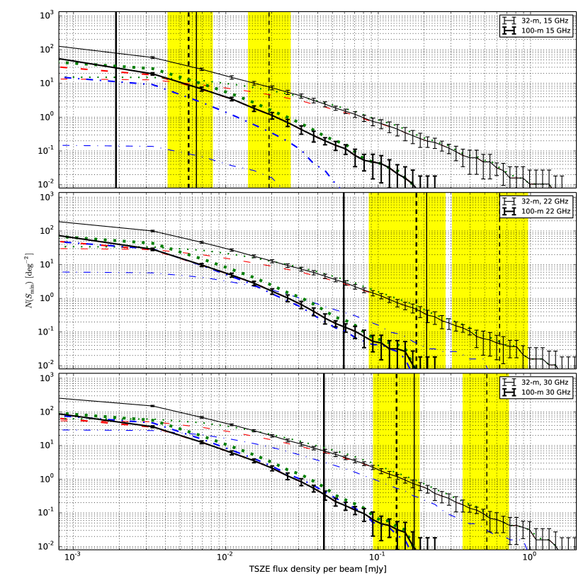
Figure 13: Predictions for the number, $N(S_{\mathrm{min}})$, of galaxy clusters per $\rm deg^{2}$ detectable through their TSZEs above a given flux density limit, $S_{\mathrm{min}}$ (eq. 25). The three panels correspond to operation at $15$, $22$, and $30$ GHz. In each panel the thick lines correspond to the cluster count expected for the 100-m RTH telescope and thin lines correspond to the 32-m telescope. Solid (black) lines with error bars show $N(S_{\mathrm{min}})$ due to TSZE only calculated for individual halos, with the $\pm 1\sigma$ sample variance – ignoring halo alignments and radio source contamination. Dashed (red) lines trace the counts after filtering out halos with angular virial diameter less than the HPBW of the corresponding telescope/receiver combination. Dotted (green) lines show the further change caused by TSZE flux density confusion, from the superposition of clusters near the line of sight. Dash-dotted (blue) lines show the additional impact of the synchrotron radio source population with flux-densities above 100$\mu$Jy, which effectively cancels part of the TSZE flux density. The vertical solid lines indicate the RMS noise level for the telescope/receiver combination, and the vertical dashed lines mark the $3\,\times$ RMS flux density level for candidate TSZE detections. The shaded (yellow) regions encompass the $\pm 3\sigma$ confidence ranges in the theoretically achievable $S_{\mathrm{min}}$ corresponding to seasonal and elevation-dependent variations of system performance.

V.3.1 Scale dependence and redshift coverage

It is of interest to investigate the range of redshifts of clusters from TSZE surveys, since clusters selected in this way are expected to cover a wide range of redshifts, and so to provide excellent objects for testing our understanding of the growth of structure. In figure 14 we show the population of clusters expected from 32-m/30-GHz and 100-m/15-GHz surveys as functions of halo mass (and virial angular size), and redshift, based on seven deep-field realisations. Halo TSZEs are placed on the figure ignoring confusion from the primordial CMB and halo alignments, but the level of CMB confusion is indicated as a curve of flux density noise per beam, calculated from

$$\Delta S(\nu,\theta_{b})=[B_{\nu}(T_{\mathrm{CMB}})-B_{\nu}(T_{\mathrm{CMB}}+\Delta T)]\int P_{b}(\hat{\mathbf{n}})\operatorname{d}\!{\Omega}$$ (26)

where $B_{\nu}(T_{\mathrm{CMB}})$ is given by eq. 9 and $P_{b}(\mathbf{\hat{n}})$ is the aperture- and frequency-dependent instrumental beam profile. The angular dependence of CMB intensity is approximated by a simple 1:1 mapping between multipole component $\ell$ and angular scale, $\theta(\ell)=2\pi(2\ell+1)^{-1}$, with the temperature contribution on that scale $\Delta T_{\ell}=\left[\frac{1}{4\pi}(2\ell+1)C_{\ell}\right]^{1/2}$ where $C_{\ell}$ is the amplitude of the power spectrum at multipole $\ell$. By analogy, the cumulative contribution from all scales less than $\theta$ is calculated as $\sigma^{2}_{\ell_{\mathrm{min}}}=\sum_{\ell=\ell_{\mathrm{min}}}^{\ell_{\mathrm{max}}}\sigma^{2}_{\ell}$ where $\ell_{\mathrm{max}}=6000$ is the highest multipole in the calculated power spectrum. The corresponding CMB noise is plotted in figure 14 as black solid lines: for most halos detectable in the planned surveys this noise is small because most of the halos lie at high redshift, and so have small angular scales, where the primary CMB fluctuations become exponentially damped.

For the RT32/OCRA-f configuration halos with virial angular scales between 3 and 30 arcmin are the most likely to be detected (at $3\sigma$ confidence), and these lie in redshift range $0.03\lesssim z\lesssim 0.5$. The flux density peak is found at redshift $z\approx 0.1$, and none of the halos with detectable flux density has an angular scale smaller than the beam size.

In the case of RTH with the 49-beam Ku-band array, the most likely virial angular scales are between $0.3$ and 30 arcmin, and clusters out to $z\approx 2$ could be detected. The predictions of the telescope selection functions in terms of the detectable cluster mass and redshift (figure 14) are based on a theoretical sensitivity limit (section V.2) and the integrated TSZE flux-densities but without the impact of point sources. We did not investigate the impact from individual effects jointly as it would require extrapolations below the experimentally probed range of radio source flux-densities (section III.7.1). Note that the bottom panels of figure 14 do not readily show the number of clusters above certain flux-density limit because the plotted $S-M_{\mathrm{vir}}$ scaling relation combines several FOV realisations.

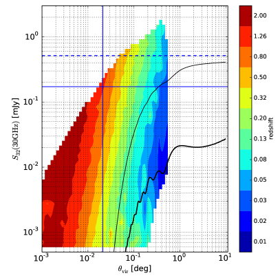
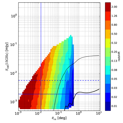
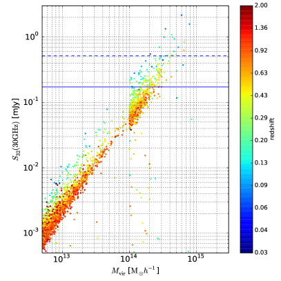
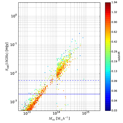
Figure 14: Distribution of TSZE flux density per beam from single halos as a function of halo virial angular size (upper row) and virial mass (lower row), with redshift indicated by the colour scale. The left column shows the halos that could be detected by a 32-m telescope at 30 GHz. The right column is for a 100-m telescope at 15 GHz. Horizontal lines indicate the same flux density thresholds as in figure 13. The thin black curves in the top row indicate the $1\sigma$ rms level of the flux density (per beam) variation from CMB fluctuations as a function of angular scale (see text for details). The thick lines indicate the CMB flux density per beam from all angular scales $<\theta_{\mathrm{vir}}$. The effects of the halo superposition and point source confusion are not included. The filled contours in the upper row show the statistics of the halo redshift distribution. The lower plots show individual halos. The distribution of halos in the $\theta_{\mathrm{vir}}-S$ plane is not uniform: there are more halos with low TSZE flux densities than high flux densities. For clarity, only 2% of the halos with virial mass of $<10^{14}M_{\odot}/h$ are shown in the lower plots.

The number of galaxy clusters detected in a blind survey depends mostly on the observing frequency, the beam size, and the system sensitivity. At centimetre wavelengths, increasing the observing frequency makes the TSZE specific intensity larger, but the telescope beam smaller, on any given telescope. The first factor causes only a weak redshift dependence (related to cluster temperature evolution), but the second factor scales with the square of the angular diameter distance, and hence is a rapid function of redshift.

Figure 14 shows that at the virial overdensity, clusters larger than $\sim 0.5^{\circ}$ are very rare, and although they may be very massive, with large total flux densities, they do not necessarily yield the largest flux density per beam as the TSZE signal is strongly non-uniform – peaking at the cluster core and decreasing towards the cluster outskirts. Such rare objects are not well represented in our simulations, and more precise predictions of their numbers in the widest-area surveys requires a much larger simulated field — a calculation which we defer to the future. For the present, we note only that the sampling noise at the lowest redshifts is significant, as is apparent from the small number of clusters with $M_{\rm vir}>4\times 10^{15}M_{\odot}h^{-1}$.

The statistics of the halo distribution plotted in Figure 14 is based on the selected FOV but the we argue that the result is quite general. While the flux density and redshift distribution are independent from the FOV, the total number of clusters in the light-cone would change when the FOV was chosen to be slightly smaller or larger from the one in our simulation, but the relative proportions of cluster counts at different redshifts should be conserved yielding similar statistics under assumption of statistical isotropy.

V.3.2 The effects of limited angular resolution

Finite beamwidth leads effectively to a cut-off in the distribution of detectable TSZE galaxy clusters and causes flattening in the cumulative $N(S_{\mathrm{min}})$ distribution in the limit of high redshift and so small flux density (red dashed lines in figure 13). The halo filtering criterion depends on the observing strategy used: beam-switching techniques, for example, also imply a cutoff at low redshift and so high flux density (Birkinshaw (1999)). Detailed planning of the survey methodology is required to investigate these effects for the planned RT32 and RTH surveys, but a fair approximation for the total number of detectable halos can be obtained by adopting the criterion that $\theta_{\mathrm{vir}}>\theta_{b}$: i.e., that the angular virial size of a halo should exceed the observing HPBW, and that criterion was used in figure 13).

An objection to this procedure may be found from the results of the Planck satellite (Planck Collaboration et al. (2011)). Most of the cluster candidates detected by Planck through their TSZEs correspond to halos smaller than the Planck beamwidth. However, ground-based observations are limited by strongly structured and powerful atmospheric noise, and we expect it to be difficult to detect clusters smaller than the beam size.

V.3.3 The effects of halo LOS alignment

A second effect caused (in part) by limited angular resolution is confusion of halos by superposition on the line of sight.

The additive nature of TSZEs from multiple halos on the line of sight is evident in figure 11: the bottom-right panel displays many examples of small angular size (distant) TSZEs superposed on more extended (lower-redshift) clusters. Halo alignments lead to boosted TSZE flux density per beam, with the flux density of maximum boosting being a function of the beam size and the distribution of halos in redshift. Effectively, the TSZE flux density detected from a halo is increased while the number of halos is unchanged. Thus in figure 13 the green (dotted) lines that display the effects of halo alignment lie above the red (dashed) lines that show the effect of beam size selection of individual halos. The two sets of curves converge at low flux densities because of the halo filtering criterion.

Halo LOS alignments change the apparent count of detectable clusters in our statistics by an amount smaller than sample variance for 22- and 30-GHz surveys with either the 32-m or 100-m telescopes. However, at the lower flux density threshold achievable with the 49-beam radio camera on the 100-m telescope there is a significant impact, and a TSZE flux density bias should be taken into account when reconstructing scaling relations at the faintest flux density levels, of order $100\ \rm\mu Jy$ or less.

V.3.4 The effects of unresolved radio sources

Unresolved radio sources appearing near the line of sight to a halo will decrease the integrated TSZE flux density of that halo. This effect is shown in figure 13 by the dash-dotted (blue) lines. These lines result from integrating specific intensity FOV simulations that include TSZEs from all identified and reconstructed halos (section III) and from simulated radio sources brighter than $100\mu$Jy (section. III.7.1), using the instrumental beams given in table 1. The statistics obtained from different light-cone realisations account for TSZ–radio-source cross-correlations, but in this calculation we ignore accidental correlations with the primordial CMB.

Although massive halos tend to have more contaminating sources (see Section III.7.2), a low redshift survey with a small beam makes it easier to clip out the affected source regions, and so reduce the confusion that would be obtained with a smaller telescope or lower frequency.

The strength of the clustering of radio sources towards massive halos is key in quantifying the flux cancellation. In the present work we use a free parameter, calibrated by point-source/galaxy-cluster associations. However, the source distribution is complicated, and the description of the source properties that we use is a relatively simple approximation (see section III.7.2). While the mean overdensity of radio sources towards known clusters can be assessed from our cross-correlation analysis, the radial density profile, richness-mass relation, and radial spectral variations in the source population should also be taken into account. Our current approach weights the spatial radio source PDF by cluster mass, but the masses of the clusters used in the cross-correlation analysis are not known. Instead we assign 2D PDF contributions based on the masses of halos that happen to be in the simulated FOV. The contribution of clustered sources relative to the uniformly-distributed source component may be over- or under-estimated depending on the extent to which the halos in the simulated FOV correspond to the masses of the clusters used for the cross-correlation analysis. A more detailed analysis of the clustering properties of radio sources will be possible as a consequence of the surveys that we plan, and will allow better-tuned modelling of the source contents of clusters. Although there is a possibility that, at the lowest radio-source flux densities, a uniformly-distributed radio-source population with a central void could mimic the TSZE, in the present work we do not seek such configurations as we only measure TSZE flux density towards known halos. These cases however, along with a possibility of spurious detections due to presence of various noise components, will be quantified when the final source extraction algorithms are developed. However, this is beyond the scope of the present work.

Radio sources have most impact on TSZE flux density measurements at lower frequencies, for a given radio telescope, due to the larger beam as well as the brighter synchrotron radiation. At a fixed frequency, the impact of radio sources can be mitigated only by observing with a larger telescope.

V.3.5 Low-mass halo contributions to the LOS integrated Compton $y$-parameter

Typically there are about $4\times 10^{4}$ halos (with at least $N_{h}=600$ SPH particles per halo; see Section III.1) in the simulated deep field. Such a value of $N_{h}$ could lead to an underestimation of the calculated TSZE flux density distribution because the lighter halos are neglected, but are abundant because of the steepness of the halo mass function, and so could contribute significantly to the sky distribution of the Compton $y$ parameter.

We have investigated the LOS contribution of halos up to a factor $10$ in mass below our normal limit by decreasing $N_{h}$ to $60$ (corresponding to mass scale $M_{h,\rm min}\approx 1.3\cdot 10^{12}M_{\odot}h^{-1}$, or about the mass of a large spiral galaxy), recalculating the Compton $y$-parameter map, and then examining the strongest peaks in difference from our basic map. The reduction in $N_{h}$ raises the typical number of halos to more than $6\times 10^{5}$, but the $y$-parameter is increased by few per-cent at the most, towards the halos selected using $N_{h}\geq 600$ condition.

We conclude that the LOS contribution of light halos is statistically unimportant and typically $\ll 10\%$. The underlying reason stems from chances of LOS alignment and also from the fact that these lighter halos have lower temperatures and densities, and smaller physical sizes, than more massive halos. All three factors work in the same sense, to reduce the TSZE from a halo, and the reduction in TSZE per halo is more significant than the increase in halo numbers at low masses.

Since $N_{h}\geq 60$ halos constitute a superset of $N_{h}\geq 600$ halos there exist multiple Compton $y$-parameter peaks from halos just below the $N_{h}=600$ threshold which build structures distributed around heavier halos. Depending on the halo redshift and telescope beamwidth these may also occasionally contribute at the level of up to several per-cent.

V.3.6 Predictions for a wide field survey and impact of point source clustering

It is difficult to infer directly the number of detectable TSZE galaxy clusters in the PISKY field from the simulated deep field, because of high Poisson noise on the abundance of the most massive halos. However, figure 14 (bottom-right panel) shows that for the $3\,\times$ RMS flux density threshold (0.79 mJy) derived for the RTH’s PISKY survey (table 3), a detectable TSZE signal will arise from a cluster mass $\sim 2.2\times 10^{15}M_{\odot}/h$. Assuming that only the nearby (low redshift) galaxy clusters will be massive enough to yield that requirement, and using the reconstructed FOF mass function depicted in the figure 7 we estimate that there are $17^{+15}_{-8}$ $\mathrm{Gpc^{-3}}$ (68% CL) galaxy clusters within the FOF mass range $(1.8,3.2)\times 10^{15}$ $\mathrm{M_{\odot}}/h$. For the cone-like PISKY field survey with the assumed opening angle of 120 deg, and depth reaching redshift $z=1.0$, the corresponding comoving volume $V=39.2$ Gpc³ by a simple rescaling would contain $N_{PISKY}=676^{+612}_{-321}$ clusters (68% CL). Thus, given the mass-TSZE flux-density relation (figure 14) it should be expected that deepening this survey in a multi-year campaign would quickly increase the detectable cluster’s count. This result, however, still needs to be corrected for the presence of point sources. Accurate predictions for the wide and shallow survey are difficult, as the degree of clustering has a strong effect, and Figure 13 shows that, at 15-GHz, point source confusion is increasingly significant at higher halo masses (higher flux-densities), and that point sources effectively decrease the halo counts by a factor of $>10$ at 0.1 mJy for the assumed clustering level. We recalculated the statistic for the case of non-clustered sources and found that the effective TSZE counts are less suppressed, as expected. In our simulations the clustering is frequency independent, and the impact on the counts results only from frequency-dependent beamwidths. The suppression in the total TSZEs counts due to switching from the non-clustered to the clustered case is largest at low frequencies giving a ratio of $\sim 10$ ($\sim 1.6$) at 15 GHz for RT32 (RTH). At 30 GHz the overall impact on the count ratio is small: $<1.2$ for both RT32 and RTH. However, the angular clustering PDF peak amplitudes are proportional to halo masses and so perhaps a more significant impact of clustering is seen at the highest masses — which is the most interesting from the observational point of view. In the high mass limit, and in the non-clustered case, the effective cluster count curves for RTH approach the green (dotted) lines in Fig. 13 – the counts without the effects of point sources for all frequencies. RTH at 30 GHz would be, in principle, immune to variations of point source clustering.

Details of the point source clustering therefore do have impact on detectable cluster counts predictions in the PISKY survey. We estimate the effective cluster count as $N_{PISKY}*f$ up to a multiplicative factor $f$. $f$ ranges from $\sim 1$ in the non-clustered case to $<0.1$ for the case of clustering assumed in our simulations hence, the resulting effective cluster count will be of order $O(10)$.

Less confusion is observed at higher frequencies (smaller beamwidths), but the penalty is a decreased survey depth (for a duration-fixed survey). A 4-year PISKY survey would have TSZE flux density limit 1.8 mJy ($3\times$ RMS) if the 49-beam camera of RTH was operating at 30-GHz. As pointed out in section V.1 the integrated TSZE flux density changes as square of beamwidth which, in turn, shifts the $N(S_{\mathrm{min}})$ distribution towards smaller flux densities and effectively increases the cluster mass required for successful detection to $\sim 10^{16}M_{\odot}/h$ for a 30-GHz PISKY survey with RTH. Since galaxy clusters generally have mass less than $10^{16}M_{\odot}/h$,it is clear that large apertures surveying fields that are very wide and very shallow and at an increased frequency will not guarantee many detections. This makes SZ observations challenging, since at larger beamwidths the only way to effectively detect TSZE is to either use very large cameras and/or have a better receiver performance and stable atmospheric conditions.

V.3.7 Frequency and receiver-telescope dependence

In Table 3 we report that at 15 GHz RTH will statistically detect $4^{+2}_{-2}$ clusters per year in a SQDF above $3\times\mathrm{RMS}=6\mu$ Jy. Figure 15 summarises the flux density relations under change of observational frequency and telescope-receiver configurations. In this section we investigate the case of 30-GHz (no beam-switched) 49-beam receiver with the same receiver noise level and bandwidth as OCRA-f if installed on RT32. The TSZE survey limit after 1-year (4-year) of operation would be $\sim 0.1$ mJy (0.05 mJy) and within the SQDF survey it would effectively detect 0.9 ($\sim 2.5$) clusters per square degree. Within this regime this shows that it is slightly more effective to keep constant survey depth and increase survey area after reaching the initial depth. The effective cluster detection rate would be then $\sim 4.2$ times lower than in the case of 15-GHz camera on RTH, the TSZEs loss due to point sources would be similar, but the survey would find much stronger TSZE flux densities – tens-to-hundreds of times stronger – which could turn out to be more feasible than the low frequency survey.

If the RTH camera were to operate at the higher frequency of 30 GHz it would provide a better signal/noise ratio and would detect stronger TSZEs with superior angular resolution. As pointed out in earlier sections, such a configuration results in a TSZE distribution shifted towards smaller flux densities per beam, but the advantages of a larger beam in terms of integrated signal should be recovered with data smoothing, and point source excision, during data analysis.

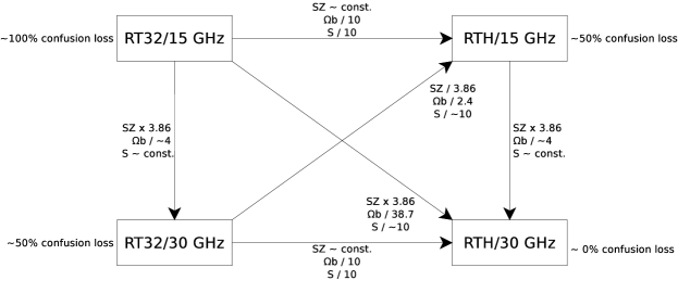
Figure 15: A diagrammatic and simplified representation of approximate relations between the TSZE intensity (marked as SZ), telescope beam size $\Omega_{b}$ and TSZE flux per beam (S) under changes of observing frequency and telescope aperture. Within the same frequency the amplitude of TSZE remains constant. The ’$\times f$’ (’$/f$’) indicates an increase (drop) of a quantity by a factor $f$ under the configuration change indicated by the corresponding arrow. The diagram explains the mutual relations of $N(S_{\mathrm{min}})$ distributions in Figure. 13. For each telescope–observing-frequency combination an approximate fraction of TSZEs lost to radio-source contamination is also indicated.

V.4 Predictions for blind point source surveys

In this section we calculate the total number of radio sources that we expect to detect in blind surveys to flux density threshold $S_{\mathrm{min}}$. Our results are summarised in figure 16, where the $N(S_{\mathrm{min}})$ distributions are shown for each of the surveys described in table 3.

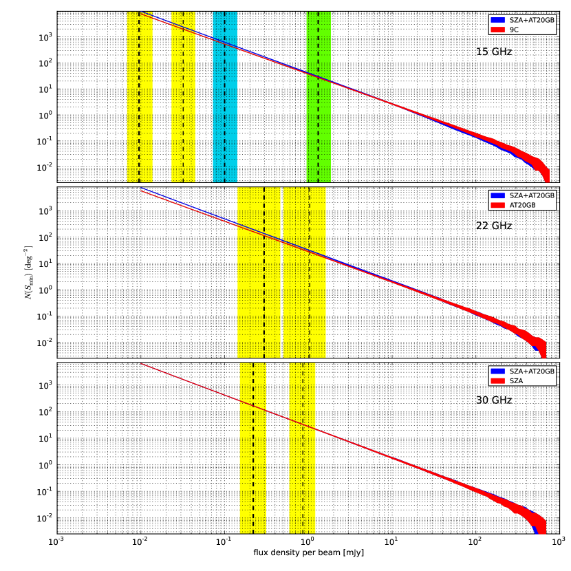
Figure 16: Predictions for the total count of radio sources, $N(S_{\mathrm{min}})$, above flux density threshold $S_{\mathrm{min}}$ (eq. 25). The three panels correspond to frequencies $15$, $22$, and $30$ GHz. In each panel thick vertical lines relate to surveys with the 100-m RTH telescope and thin lines to surveys with the 32-m telescope. The shaded regions represent 68% confidence limits based on 100 Monte-Carlo realisations of a large sky area. For each frequency we show two sets of predictions: one based on a combination of the SZA and AT20B catalogues, and one based on the single catalogue that most closely matches the planned survey frequency. Vertical dashed lines indicate the $5\,\times$ RMS flux density level expected for the SQDF surveys. Yellow shaded regions show the variation in the $5\sigma$ confidence range corresponding seasonal variations of the system performance. Flux density thresholds for the PISKY and RTHDF surveys, as defined in table 3, are shown by the green and cyan shaded regions in the top panel.

At each of the survey frequencies we compare the predicted source counts based on two different datasets. The first prediction is derived from the SZA and AT20GB surveys, combined and processed as described in section III.7.1. For the second we choose the survey performed at the frequency closest to the frequency of interest. In either case the predictions were made at the relevant survey frequency. Figure 16 shows that the different predictions are in good agreement, except at low flux densities, below the range probed by the 9C and AT20GB surveys. One of the aim of the planned surveys is to provide a large sample of sources in this sub-mJy flux density range, where the differences in the predicted source counts reflect uncertainties in the contributing source populations.

V.4.1 The effects of point source confusion

The deepest surveys with a given instrumental configuration are limited by confusion. The confusion limit is usually discussed based on some limiting number of sources per beam: at some assumed source density, such as three beams per source, the corresponding flux density is taken as the effective confusion level. This approach ignores the spatial correlations of radio sources and the contribution of sources below the adopted flux density limit. Both shortcomings underestimate the level of confusion.

In this work we derive the confusion limits in an alternative way that alleviates these problems. We calculate the confusion limit via the relative flux density measurement error, $\delta_{\mathrm{conf}}$, as

$$\delta_{\mathrm{conf}}(\nu)=\frac{S_{g}-S_{m}}{S_{g}}$$ (27)

where $S_{g}$ is the flux density generated according to the recipe outlined in Sect. III.7.1, and $S_{m}$ is the flux density measured from the high-resolution map. $S_{m}$ therefore includes the effect of confusion. In figure 17 we show $\delta_{\mathrm{conf}}(\nu)$ for the two radio telescopes for all three frequencies as a function of $S_{g}$.

Dashed and solid lines show the upper 68% (95%) percentile points for the distribution of $\delta_{\mathrm{conf}}$ — we base the confusion level as given in table 3 on the flux density at which the 68% (95%) percentile contour crosses the line $\delta_{\mathrm{conf}}=10$%. That is, at the confusion levels quoted in the table, 32% (5%) of the flux densities will have errors $>10$%.

In figure 17 we also plot contours of constant point source density distribution in the $\log\delta_{\mathrm{conf}}-\log S$ plane in order to visualise the effects of confusion when approaching the low flux density levels. In case of no confusion the sources should group horizontally along the $\delta=0$ line. In case of non-zero confusion the sources will occupy $\delta>0$ regions with the amplitude of the deviation depending on the initial flux-density and clustering properties.

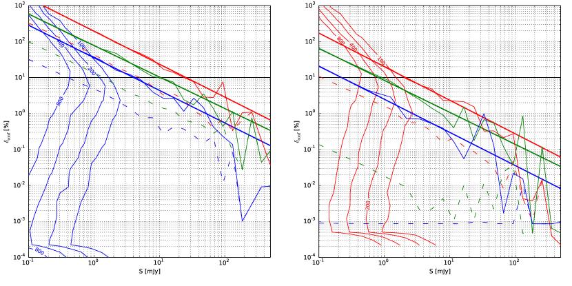
Figure 17: Radio source flux density confusion for RT32 (left) and RTH (right). Solid lines and dashed lines connect the 95% and 68% upper-tail percentiles, respectively, of the $\delta_{\mathrm{conf}}$ distributions. Linear fits (in log-log space) to the 95% distributions are shown: these approximately follow power-laws of the form $\delta_{\rm conf}\propto S_{g}^{-0.9}$. From top to bottom, the red, green, blue lines correspond to frequencies of 15, 22, and 30 GHz. The intersection of the horizontal line at $\delta_{\mathrm{conf}}=10$% with the fitted lines defines the flux density at which less than 5% of sources in the field have a systematic flux density measurement error larger than 10%. We use this as our definition of the confusion level, and summarise the values for the different telescopes and operating frequencies in table 3. The contours show the densities of radio sources in the $\delta_{\mathrm{conf}}-S$ plane (in the same, but arbitrary, units in both plots) for the RT32 at 30’ GHz (left) and for the RTH at 15 GHz (right).

VI Discussion

Our simulations have neglected AGN and star formation feedback and radiative losses, so that the M-T scaling relation (figure 9) lies below the scaling relations from observations or simulations that include more physics. Nevertheless, the predictions for the detected TSZE galaxy cluster count do not represent lower limits, but quite the opposite, as can be seen from the M-Y scaling relation (figure 10).

We speculate that one of possible sources of scatter in the scaling relations is the assumption that our estimates for $r_{\delta}$, which are well-defined for spherically-symmetric clusters, are only approximate indications of mass in the typically-asymmetrical density distributions of realistic halos at the usual values of $\delta$ (see figures 3 and 4). The implicit uncertainty propagates to quantities that depend on overdensity which are extracted from the reconstructed temperature and mass profiles. If a galaxy cluster is going through a merger event, then its temperature and mass profiles may well be irregular, and we should not even expect the density profile to fall monotonically with distance from the cluster centre. We mitigate against these problems somewhat, by fitting scaling relations using only the most massive halos, which should have more relaxed and well-defined density profiles.

The relative errors of the SPH interpolations, which we use heavily to construct the 3D $T_{\rho}$ distributions, is of the order of 1% in the signal dominated regions and depends on the chosen number of SPH neighbours. Although for the main results we use a fixed number of neighbours, $N_{\mathrm{neigh}}=33$, we might be able to improve the physical accuracy of the simulation by relating this number to the halo mass, and so to the number of SPH particles contained in the halo. We have not investigated the impact of changing from a fixed number of neighbours. For well-mixed CDM and baryon fluids we would expect the effect to be unimportant, but some differences may arise in cases where baryons are spatially separated from the CDM component, such as when baryonic gas is concentrated towards the centre of an extended CDM halo. In that case one would expect larger smoothing lengths in the central regions for a fixed $N_{\mathrm{neigh}}$ as compared to the smoothing lengths calculated for a fixed mass enclosed within the smoothing length.

The simulation mass resolution affects the amplitude of the $M$-$Y$ scaling relation (figure 10), and a simulation with a larger number of particles would result in better estimates of halo quantities at high overdensity, where most of the TSZE signal arises. While our scaling relations show that the process of computing Compton $y$-parameter profiles is relatively unaffected, we found that the $M_{500}-Y_{500}$ scaling relation amplitude is sensitive to the simulation mass resolution. Convergence at high density thresholds requires better mass resolution than we were able to undertake, but we quantified the effect by a sequence of simulations with $(N,L[\mathrm{Mpc}])=\{(256^{3},512),(512^{3},512),(256^{3},128)\}$, where $N$ is the number of particles and $L$ simulation box size. We found that the $M_{500}-Y_{500}$ scaling amplitude decreases, from $Y_{14}=6.62$ to $6.03$ and then $Y_{14}=5.61$ as the resolution increases, for a fixed number of neighbours.

Our $M$-$T$ relation (figure 9) shows that adiabatic simulations yield the scaling relations amplitude, $T_{15}$, offset by a few tens of percent from the observational amplitude. The value of amplitude depends on the smoothing length parameter used, or equivalently to the number of neighbours used in the SPH density calculations. For a fixed mass resolution, larger smoothing lengths tend to increase the amplitudes of the $M$-$Y$ and $M$-$T$ scaling relations, but we found that increasing $N_{\mathrm{neigh}}$ cannot correct for this $\sim 30$ % discrepancy. Increasing $N_{\mathrm{neigh}}$ from 33 to 66 with $N_{h}=600$ increases the value of $T_{15}$ by only about 3%. Decreasing $N_{\mathrm{neigh}}$ has a larger effect and exacerbates the discrepancy with observations. Future improvements will investigate changes in the smoothing scheme and how they might improve our results. Similarly, we showed that our results have converged well: doubling the grid resolution (from the 50 kpc value assumed here) has negligible effect, of order 1% in the $M$-$Y$ scaling relation. Extra physics, describing cooling and heating, is needed to reproduce the observed scaling relation more closely. We therefore consider our predictions for TSZE detections to be upper limits.

The most massive low-redshift clusters in the simulations have central Compton $y$-parameters of order $10^{-4}$, which corresponds to TSZE decrements of order $\mathrm{mK}$ in the Raleigh-Jeans regime. There are at few such clusters found in any $5.2\times 5.2\ \rm deg^{2}$ simulation (figure 11). Thus tracing the distribution of $y$ in the cosmic population of halos requires wide surveys, and hence large radio cameras if the survey is to be conducted in a modest time. TSZE observations are therefore challenging, and are further limited, for a blind survey at a single frequency, by the lack of filtering methods that could reduce the effect of confusion from primary CMB fluctuations (figure 14) and, more importantly, from radio sources. Once again, figure 14 emphasises that wide fields of view are required to find significant numbers of clusters with strong TSZEs, reaching mJy flux densities at the survey frequencies.

The vertical lines in the figure 13 do not monotonically increase towards higher flux density levels with the frequency. Rather, the worst sensitivity is seen at about 22 GHz. This results from the strength of the atmospheric water vapour feature that peaks at about 22 GHz and for the small number of beams available in the receiver. The substantially improved sensitivity for the 15-GHz surveys stems mainly from the large number of channels in the RTH camera.

Given the scaling relations exhibited by our mock maps, as derived in sections IV.3 and IV.4, it could be possible to roughly correct the simulations for missing or imprecise physics by multiplying the integrated Compton $y$-parameters by a halo-mass dependent factor that relates the temperatures and $Y^{\mathrm{INT}}$ from our simulations to those containing more gas physics and assumptions about heating mechanisms. A simple scaling, however, would not suffice as non-adiabatic processes alter both the amplitudes and the shapes of the temperature and Compton $y$-parameter profiles. In the present paper we choose not to attempt the correction, and accept systematic errors in our predictions that we expect to be of order 10 per cent (sections IV.3 and IV.4).

As a result of the planned, tiered RTH surveys, an interesting clue on AGN feedback activity in the most massive galaxies, and its relation to the state of the intra-cluster medium, should partially come from measurements of redshift and flux-density distributions of radio galaxies and radio-loud quasars at sub-mJy flux-density levels where spatial comoving number density decline is expected at $z\gtrsim 2$. Such a high-frequency radio survey will complement the low-frequency counts, will help to quantify the flux-density and redshift dependent ratios between flat, steep and inverted spectrum populations, will track contributions of starburst galaxies and will provide reliable flux-density extrapolations into mm-wavelengths (de Zotti et al. 2010, and references therein).

According to recent Planck results, the low-redshift cluster counts data favour a lower normalisation of the matter power spectrum than the high-redshift CMB(+lensing) data (Planck Collaboration et al. 2014c, a). This tension can be reconciled by increasing the mass of active neutrinos or by introducing a massive sterile neutrino that would suppress the small scale fluctuations with respect to the standard $\Lambda$CDM model (Wyman et al. 2014; Planck Collaboration et al. 2014c). The one-dimensional constraint on $\sigma_{8}=0.77\pm 0.02$ reported in Planck Collaboration et al. (2014c) from Planck SZ+BAO+BBN can also be reconciled with the CMB data by introducing mass estimate biases of about 40% in the reconstructed Y-M scaling relation. Interestingly, Evrard et al. (2008) reports that high normalisation values – that are now more compatible with the current CMB data – are also preferred based on analysis of the $\Lambda$CDM model halo space density as a function of dark matter velocity dispersion. In this context our chosen value could be a reasonable assumption. The currently available CMB data combined with external priors yield maximum likelihood $\sigma_{8}$ estimates that can differ between each other by as much as $\Delta\sigma_{8}\approx 0.1$ (Hou et al. 2014; Hinshaw et al. 2013) in cosmologies with massive neutrinos. Since for our main results we chose $\sigma_{8}=0.821$ (section III) we test the impact of using a different value from the one preferred by the CMB data in the concordance $\Lambda$CDM model. We test other observationally motivated normalisations using constrained, lower mass resolution simulations and PS mass functions (figure 7). Using PS mass function predictions for $\sigma_{8}=0.77$ ($0.90$) we estimate that the spatial halo density would be decreased (increased) by a factor of about $\sim 2.0$ ($\sim 2.6$) at the cluster-size mass scale with respect to the abundances used in our analyses. Using reconstructed mass functions from constrained simulations we find that the impact is somewhat smaller (due to the smaller steepness). In particular, we estimate that a decrease (increase) of $\sigma_{8}$ to the value 0.77 (0.90) would result in decreasing (increasing) the halo abundances by a factor of $\sim 1.6$ ($\sim 2.1$) for the cluster-mass halos ($\sim 1.3\times 10^{15}M_{\odot}/h$). The difference due to Planck CMB preferred normalisations is insignificant, but clearly the overall variation of the halo abundance is a quite rapid function of the chosen normalisation in this mass regime, thus making halo counts an interesting cosmological test. Further progress in the field will certainly reveal the nature of this interesting dichotomy in the observed normalisation values favoured by different data, be it due to cluster mass biases, impact of massive neutrinos or yet another process.

VII Conclusions

We have used adiabatic hydrodynamical simulations to predict the number of galaxy clusters detectable via the thermal Sunyaev-Zeldovich effect (TSZE) in a set of blind simulated surveys to be performed with the existing 8-beam, beam-switched, OCRA-f radiometer on the 32-m radio telescope in Toruń (Poland), and with the planned 100-m radio telescope Hevelius equipped with a 49-beam focal plane radio camera. Based on existing radio source surveys, we have also calculated the number of radio sources detectable in these surveys.

We analysed the effects of halo–halo and halo–radio-source alignments on the integrated flux density and count of detected TSZEs, and calculated the redshift distribution of the detectable clusters, in the presence of radio source clustering in the halos. By cross-correlating the NVSS survey with the Planck SZ cluster candidate sample we found that statistically there is roughly a ten-fold increase in the point source density towards massive clusters as compared with directions away from the cluster centres, although the value is a function of survey depth, cluster mass, and redshift range.

We visualised the improvements in the receiver sensitivity, detections count and available survey area resulting from using a large dish, and large radio cameras when carrying out blind surveys, by analysing a number of receiver-antenna combinations for frequencies from 15 to 30 GHz, taking account of the weather effects.

We used a set of high-resolution mock maps of the signals sought (section V.1) including (i) the CMB primary fluctuations; (ii) TSZEs; and (iii) the radio source population. In future these maps will be used to test the image reconstruction procedures from simulated observations, taking account of realistic atmospheric brightness instabilities and receiver performance. This process will also generate completeness functions for the interpretation of the survey results.

Based on our simulations, we showed RT32/OCRA-f will be capable of detecting $33^{+17}_{-11}$ radio sources above $0.87$ $\mathrm{mJy}$ at $5\sigma$ CL at 30 GHz in a square degree field every year, taking account of the Polish climate. The relative flux density measurement error due to background point sources is constrained to be at the level $\lesssim 8\%(66\%)$ in 68% (95%) of the detected radio sources. It is unlikely that such a survey will detect any galaxy clusters, even at $3\sigma$ CL, since the expected source density is $0.03^{+0.02}_{-0.01}$ $\mathrm{deg}^{-2}$. The main limitations of the survey arise from observing time constraints, the small number of feeds, and confusion from radio sources. Reducing the detection confidence to $2\sigma$ would result only in a modest increase of the number of detectable clusters, to $\approx 0.07$ $\mathrm{deg}^{-2}$. Therefore OCRA-f (apart from surveys for radio sources) is best-suited to small-field mapping of candidate galaxy clusters from X-ray surveys, optical/IR surveys, or Planck selections.

On the other hand, the planned 100-m radio telescope Hevelius (RTH) equipped with (initially) 49 beams and wide bandwidth horns and operating up to $\sim 22$ GHz, should be suitable for blind TSZE surveys centred around 15 GHz. Given the spectrum of TSZEs, this particular frequency is a compromise due to climate conditions at RTH’s location (giving a high frequency constraint) and radio frequency interference (giving a low frequency constraint). Taking account of confusion from radio sources, and ignoring systematical effects, we would expect RTH to detect $<4$ galaxy clusters per year in a square-degree field at $3\sigma$ CL above $6$ $\mathrm{\mu Jy}$ TSZE flux density with a field coverage of $1.5^{2}$ beam per pixel, and $<1.5$ clusters per year (at $3\sigma$ CL) in the $\approx 60$ $\mathrm{deg}^{2}$ field, above TSZE flux density of $60$ $\mathrm{\mu Jy}$ with field coverage of $2^{2}$ beam per pixel (table 3). The reason for such a low detection rate stems from radio source emission which dominates at low frequencies and even though the beam size of a 100-m telescope at 15 GHz is smaller than that of 32-m telescope at 30 GHz, in the latter case the confusion is significantly smaller while TSZE is larger. Therefore although increasing observational frequency would result in fewer counts per square degree for a fixed duration survey, it would select stronger TSZEs in the range of hundreds of $\mu$Jy where flux measurements may be less prone to atmospheric (and gain instability) systematic effects which we haven’t included in our analysis. We also find that the angular resolution of RTH operating at 30-GHz would in principle make TSZEs detection counts statistics insensitive to point source clustering properties within the limits constrained by observations. The $\approx 60$ $\mathrm{deg}^{2}$ survey would yield nearly $34\,000$ point sources brighter than $1$ $\mathrm{mJy}$ at $5\sigma$ CL, with a relative systematic flux density error due to source confusion at the level $\lesssim 2\%(20\%)$ in 68% (95%) of the detections.

A primary goal of the planned RTH will be a new, wide-area, radio source survey. Within this survey RTH will detect nearly $3\times 10^{5}$ radio sources at $5\sigma$ CL at 15 GHz in a $\pi$-steradians (PISKY) field with flux density $>1.3$ $\mathrm{mJy}$ in a one year of non-continuous mapping (with a realistic time efficiency factor) and with the relative systematic error on the flux density measurement due to confusion with unresolved radio sources at the level $\lesssim 1.5\%(16\%)$ in 68% (95%) of cases of the detected radio sources (section II and V.4). We estimate that with the PISKY survey effectively tens of galaxy clusters within the mass range $(1.8,3.2)\times 10^{15}$ $\mathrm{M_{\odot}}/h$ should be detected with $z\lesssim 1$ however the prediction depends on point source clustering properties. Deepening this survey in a multi-year campaign would quickly increase the detectable clusters count (potentially to hundreds of clusters) even if operating at relatively low frequencies around $15$ GHz.

References

- Afshordi et al. (2007) Afshordi, N., Lin, Y.-T., Nagai, D., & Sanderson, A. J. R. 2007, MNRAS, 378, 293, eprint astro-ph/0612700
- Afshordi & Tolley (2008) Afshordi, N. & Tolley, A. J. 2008, Phys. Rev. D, 78, 123507, eprint 0806.1046
- Alam et al. (2011) Alam, U., Lukić, Z., & Bhattacharya, S. 2011, ApJ, 727, 87, eprint 1004.0437
- Arnaud et al. (2005) Arnaud, M., Pointecouteau, E., & Pratt, G. W. 2005, A&A, 441, 893, eprint astro-ph/0502210
- Bennett et al. (2003) Bennett, C. L., Halpern, M., Hinshaw, G., et al. 2003, ApJS, 148, 1, eprint astro-ph/0302207
- Benson et al. (2013) Benson, B. A., de Haan, T., Dudley, J. P., et al. 2013, ApJ, 763, 147, eprint 1112.5435
- Birkinshaw (1999) Birkinshaw, M. 1999, Phys. Rep., 310, 97, eprint astro-ph/9808050
- Browne et al. (2000) Browne, I. W., Mao, S., Wilkinson, P. N., et al. 2000, in Society of Photo-Optical Instrumentation Engineers (SPIE) Conference Series, Vol. 4015, Radio Telescopes, ed. H. R. Butcher, 299–307
- Burenin & Vikhlinin (2012) Burenin, R. A. & Vikhlinin, A. A. 2012, Astronomy Letters, 38, 347, eprint 1202.2889
- Carroll et al. (1992) Carroll, S. M., Press, W. H., & Turner, E. L. 1992, ARA&A, 30, 499
- Coble et al. (2007) Coble, K., Bonamente, M., Carlstrom, J. E., et al. 2007, AJ, 134, 897, eprint astro-ph/0608274
- Condon et al. (1998) Condon, J. J., Cotton, W. D., Greisen, E. W., et al. 1998, AJ, 115, 1693
- Dalal et al. (2008) Dalal, N., Doré, O., Huterer, D., & Shirokov, A. 2008, Phys. Rev. D, 77, 123514, eprint 0710.4560
- De Petris et al. (2002) De Petris, M., D’Alba, L., Lamagna, L., et al. 2002, ApJ, 574, L119, eprint astro-ph/0203303
- de Zotti et al. (2010) de Zotti, G., Massardi, M., Negrello, M., & Wall, J. 2010, A&A Rev., 18, 1, eprint 0908.1896
- Dunsby et al. (2010) Dunsby, P., Goheer, N., Osano, B., & Uzan, J.-P. 2010, J. Cosmology Astropart. Phys, 6, 17, eprint 1002.2397
- Eke et al. (1996) Eke, V. R., Cole, S., & Frenk, C. S. 1996, MNRAS, 282, 263, eprint astro-ph/9601088
- Eke et al. (1998) Eke, V. R., Navarro, J. F., & Frenk, C. S. 1998, ApJ, 503, 569, eprint astro-ph/9708070
- Evrard et al. (2008) Evrard, A. E., Bialek, J., Busha, M., et al. 2008, ApJ, 672, 122, eprint astro-ph/0702241
- Ferraro et al. (2011) Ferraro, S., Schmidt, F., & Hu, W. 2011, Phys. Rev. D, 83, 063503, eprint 1011.0992
- Giannantonio et al. (2014) Giannantonio, T., Ross, A. J., Percival, W. J., et al. 2014, Phys. Rev. D, 89, 023511, eprint 1303.1349
- Gingold & Monaghan (1977) Gingold, R. A. & Monaghan, J. J. 1977, MNRAS, 181, 375
- Górski et al. (2005) Górski, K. M., Hivon, E., Banday, A. J., et al. 2005, ApJ, 622, 759, eprint astro-ph/0409513
- Hernquist & Katz (1989) Hernquist, L. & Katz, N. 1989, ApJS, 70, 419
- Hinshaw et al. (2013) Hinshaw, G., Larson, D., Komatsu, E., et al. 2013, ApJS, 208, 19, eprint 1212.5226
- Hou et al. (2014) Hou, Z., Reichardt, C. L., Story, K. T., et al. 2014, ApJ, 782, 74, eprint 1212.6267
- Hunter (2007) Hunter, J. D. 2007, Computing In Science & Engineering, 9, 90
- Kaiser (1986) Kaiser, N. 1986, MNRAS, 222, 323
- Kettle & Roddis (2007) Kettle, D. & Roddis, N. 2007, in Microwave Symposium, ed. I.-S. International (IEEE), pp. 2087 – 2090
- Kneissl et al. (2001) Kneissl, R., Jones, M. E., Saunders, R., et al. 2001, MNRAS, 328, 783, eprint astro-ph/0103042
- Komatsu & Seljak (2002) Komatsu, E. & Seljak, U. 2002, MNRAS, 336, 1256, eprint astro-ph/0205468
- Lancaster et al. (2011) Lancaster, K., Birkinshaw, M., Gawroński, M. P., et al. 2011, MNRAS, 418, 1441, eprint 1106.3766
- Levenberg (1944) Levenberg, K. 1944, Quarterly of Applied Mathematics, 2, 164
- Lewis et al. (2000) Lewis, A., Challinor, A., & Lasenby, A. 2000, ApJ, 538, 473, eprint astro-ph/9911177
- Łokas et al. (2006) Łokas, E. L., Wojtak, R., Gottlöber, S., Mamon, G. A., & Prada, F. 2006, MNRAS, 367, 1463, eprint astro-ph/0511723
- Lucy (1977) Lucy, L. B. 1977, AJ, 82, 1013
- Mantz et al. (2014) Mantz, A. B., Abdulla, Z., Carlstrom, J. E., et al. 2014, ArXiv e-prints, eprint 1401.2087
- Marquardt (1963) Marquardt, D. 1963, J. SIAM, 11, 431
- Matarrese & Verde (2008) Matarrese, S. & Verde, L. 2008, ApJ, 677, L77, eprint 0801.4826
- Matarrese et al. (2000) Matarrese, S., Verde, L., & Jimenez, R. 2000, ApJ, 541, 10, eprint astro-ph/0001366
- Muchovej et al. (2010) Muchovej, S., Leitch, E., Carlstrom, J. E., et al. 2010, ApJ, 716, 521, eprint 0912.2335
- Muchovej et al. (2012) Muchovej, S., Leitch, E., Culverhouse, T., Carpenter, J., & Sievers, J. 2012, ApJ, 749, 46, eprint 1202.0527
- Murphy et al. (2010) Murphy, T., Sadler, E. M., Ekers, R. D., et al. 2010, MNRAS, 402, 2403, eprint 0911.0002
- Nagai (2006) Nagai, D. 2006, ApJ, 650, 538, eprint astro-ph/0512208
- Nagai et al. (2007) Nagai, D., Kravtsov, A. V., & Vikhlinin, A. 2007, ApJ, 668, 1, eprint astro-ph/0703661
- Peel (2010) Peel, M. 2010, ArXiv e-prints, eprint 1006.2760
- Planck Collaboration et al. (2014a) Planck Collaboration, Ade, P. A. R., Aghanim, N., et al. 2014a, A&A, 571, A1, eprint 1303.5062
- Planck Collaboration et al. (2014b) Planck Collaboration, Ade, P. A. R., Aghanim, N., et al. 2014b, A&A, 571, A16, eprint 1303.5076
- Planck Collaboration et al. (2014c) Planck Collaboration, Ade, P. A. R., Aghanim, N., et al. 2014c, A&A, 571, A20, eprint 1303.5080
- Planck Collaboration et al. (2011) Planck Collaboration, Ade, P. A. R., Aghanim, N., et al. 2011, A&A, 536, A8, eprint 1101.2024
- Press & Schechter (1974) Press, W. H. & Schechter, P. 1974, ApJ, 187, 425
- Prokhorov et al. (2011) Prokhorov, D. A., Dubois, Y., Nagataki, S., Akahori, T., & Yoshikawa, K. 2011, MNRAS, 415, 2505
- Rapetti et al. (2010) Rapetti, D., Allen, S. W., Mantz, A., & Ebeling, H. 2010, MNRAS, 406, 1796, eprint 0911.1787
- Refregier et al. (2000) Refregier, A., Komatsu, E., Spergel, D. N., & Pen, U.-L. 2000, Phys. Rev. D, 61, 123001, eprint astro-ph/9912180
- Roncarelli et al. (2010) Roncarelli, M., Moscardini, L., Branchini, E., et al. 2010, MNRAS, 402, 923, eprint 0909.4714
- Sachs & Wolfe (1967) Sachs, R. K. & Wolfe, A. M. 1967, ApJ, 147, 73
- Sadeh et al. (2007) Sadeh, S., Rephaeli, Y., & Silk, J. 2007, MNRAS, 380, 637, eprint 0706.1340
- Schmidt et al. (2009a) Schmidt, F., Lima, M., Oyaizu, H., & Hu, W. 2009a, Phys. Rev. D, 79, 083518, eprint 0812.0545
- Schmidt et al. (2009b) Schmidt, F., Vikhlinin, A., & Hu, W. 2009b, Phys. Rev. D, 80, 083505, eprint 0908.2457
- Sehgal et al. (2011) Sehgal, N., Trac, H., Acquaviva, V., et al. 2011, ApJ, 732, 44, eprint 1010.1025
- Shapiro et al. (1994) Shapiro, P. R., Giroux, M. L., & Babul, A. 1994, ApJ, 427, 25
- Springel (2003) Springel, V. 2003, http://www.mpa-garching.mpg.de/gadget/right.html
- Springel (2005) Springel, V. 2005, MNRAS, 364, 1105, eprint astro-ph/0505010
- Sunyaev & Zeldovich (1972) Sunyaev, R. A. & Zeldovich, Y. B. 1972, Comments on Astrophysics and Space Physics, 4, 173
- Tinker et al. (2008) Tinker, J., Kravtsov, A. V., Klypin, A., et al. 2008, ApJ, 688, 709, eprint 0803.2706
- Vale & White (2006) Vale, C. & White, M. 2006, New A, 11, 207, eprint astro-ph/0501132
- Van Waerbeke et al. (2014) Van Waerbeke, L., Hinshaw, G., & Murray, N. 2014, Phys. Rev. D, 89, 023508, eprint 1310.5721
- Vanderlinde et al. (2010) Vanderlinde, K., Crawford, T. M., de Haan, T., et al. 2010, ApJ, 722, 1180, eprint 1003.0003
- Vikhlinin et al. (2006) Vikhlinin, A., Kravtsov, A., Forman, W., et al. 2006, ApJ, 640, 691, eprint astro-ph/0507092
- Voit (2005) Voit, G. M. 2005, Reviews of Modern Physics, 77, 207, eprint astro-ph/0410173
- Voit (2011) Voit, G. M. 2011, ApJ, 740, 28, eprint 1107.2142
- Voit & Donahue (2014) Voit, G. M. & Donahue, M. 2014, ArXiv e-prints, eprint 1409.1601
- Waldram et al. (2003) Waldram, E. M., Pooley, G. G., Grainge, K. J. B., et al. 2003, MNRAS, 342, 915, eprint astro-ph/0304275
- Weinberg et al. (2013) Weinberg, D. H., Mortonson, M. J., Eisenstein, D. J., et al. 2013, Phys. Rep., 530, 87, eprint 1201.2434
- White et al. (1993) White, S. D. M., Efstathiou, G., & Frenk, C. S. 1993, MNRAS, 262, 1023
- Wilson et al. (2009) Wilson, T. L., Rohlfs, K., & Hüttemeister, S. 2009, Tools of Radio Astronomy (Springer-Verlag)
- Wojtak & Łokas (2010) Wojtak, R. & Łokas, E. L. 2010, MNRAS, 408, 2442, eprint 1004.3771
- Wyman et al. (2014) Wyman, M., Rudd, D. H., Vanderveld, R. A., & Hu, W. 2014, Physical Review Letters, 112, 051302, eprint 1307.7715
- Zel’dovich (1970) Zel’dovich, Y. B. 1970, A&A, 5, 84