Full analysis of multi-photon pair effects in spontaneous parametric down conversion based photonic quantum information processing

Abstract

In spontaneous parametric down conversion (SPDC) based quantum information processing (QIP) experiments, there is a tradeoff between the coincide count rates (i.e. the pumping power of the SPDC), which limits the rate of the protocol, and the visibility of the quantum interference, which limits the quality of the protocol. This tradeoff is mainly caused by the multi-photon pair emissions from the SPDCs. In theory, the problem is how to model the experiments without truncating these multi-photon emissions while including practical imperfections.

In this paper, we establish a method to theoretically simulate SPDC based QIPs which fully incorporates the effect of multi-photon emissions and various practical imperfections. The key ingredient in our method is the application of the characteristic function formalism which has been used in continuous variable QIPs. We apply our method to three examples, the Hong-Ou-Mandel interference and the Einstein-Podolsky-Rosen interference experiments, and the concatenated entanglement swapping protocol. For the first two examples, we show that our theoretical results quantitatively agree with the recent experimental results. Also we provide the closed expressions for these the interference visibilities with the full multi-photon components and various imperfections. For the last example, we provide the general theoretical form of the concatenated entanglement swapping protocol in our method and show the numerical results up to 5 concatenations. Our method requires only a small computation resource (few minutes by a commercially available computer) which was not possible by the previous theoretical approach. Our method will have applications in a wide range of SPDC based QIP protocols with high accuracy and a reasonable computation resource.

I Introduction

Spontaneous parametric down conversion (SPDC) is one of the most standard tools in photonic quantum information processing (QIP) e.g. quantum key distribution, quantum teleportation, quantum repeaters, and linear optics quantum computation Pan2012 . Toward implementing higher rate entanglement-based QKD or larger scale QIP protocols, it is important to increase the photon-pair generation rate from the SPDC source such that it provides reasonable coincidence counts of photons in multiple detectors. Though this is possible by simply increasing the pump power into the SPDC crystals, it simultaneously degrades the quantum interference visibility due to the unwanted multi-photon emissions. Therefore, on one hand, it is an important experimental topic how to reduce the effect of multi-photon emissions while keeping the higher generation rates. The experimental progress in this direction has been reported recently Kuzucu2008 ; Krischek2010 ; Ma2011 ; Broome2011 ; Jin2014SR .

On the other hand, in theory, it is desirable to establish a method which fully incorporates the multi-photon emissions and various practical imperfections of the experiment, and is also able to simulate various QIP applications with complicated optical circuits. The quantum state generated into the signal and idler modes from an SPDC source is described by a two-mode squeezed vacuum (TMSV):

$$|\psi\rangle_{SI}=\sqrt{1-\lambda^{2}}\sum_{n=0}^{\infty}\lambda^{n}|n\rangle_{S}|n\rangle_{I},$$ (1)

where $|n\rangle$ represents an $n$-photon state, and $\lambda$ is the squeezing parameter. Obviously it includes infinitely higher order photons that contribute to the multi-photon emissions. Also, to simulate experiments precisely, one has to take into account various imperfections such as losses in channels and detectors, dark counts of detectors, mode mismatch between the pulses, and so on.

The theory to describe multi-photon emissions have been investigated in various literatures Ou1999 ; Riedmatten2004 ; Scarani2005 ; Scherer2009 ; Wieczorek2009 ; Takesue2010 ; Broome2011 ; Jennewein2011 ; Sekatski2012 ; Khalique2013 ; Jin2014SR . A major approach is to calculate the evolution of the state vector of the TMSVs in the protocol Ou1999 ; Riedmatten2004 ; Scarani2005 ; Scherer2009 ; Wieczorek2009 ; Takesue2010 ; Broome2011 ; Jennewein2011 ; Khalique2013 ; Jin2014SR . Although the approach is straightforward and useful to see the physical insight of multi-photon effects, one of its drawback is that one has to truncate the higher photon number Ou1999 ; Riedmatten2004 ; Scarani2005 which is not appropriate for the higher power pumping. In principle, it is possible to include (even infinitely) higher order photons in analytical forms. However, the problem is that its mathematical expression often becomes complicated even for relatively simple setup using only one or two SPDCs like Scherer2009 ; Jin2014SR . This is more problematic for a larger scale QIP protocol. That is, its numerical simulation often require a huge computational resource even truncating the higher order of photons. This severely limits the ability to estimate the practical performance of such a protocol. For example, in Khalique2013 , the concatenated operation of entanglement swapping is theoretically investigated where the authors showed precise but highly complicated mathematical expression of the states and detection probabilities in the protocol and performed its numerical simulation for the concatenation of 3 swappings, which involves 16 optical modes. The simulation was performed by a parallel programing on a super computer meaning that it requires a huge computational resource even for that scale of the protocol. Therefore to extend the analysis for larger SPDC based QIP networks, it is desirable to find an alternative way of calculating such a problem more systematically, simply, and with less computational resources.

As a related work to the above, the authors in Sekatski2012 developed a precise mathematical model of nonideal photon detectors and then derived analytical formulae of several parameters for the experiments with one SPDC source, including the Hong-Ou-Mandel (HOM) interference and the Einstein-Podolsky-Rosen (EPR) interference visibilities where multi-photon pair effects and detector imperfections are successfully incorporated. Although their formulae are useful for the practical estimation of these experiments, it is not fully clear if the approach is easily extendible to more complicated protocols such as the concatenated entanglement swapping discussed in Khalique2013 .

In this paper, we propose yet another approach based on the phase space representation of quantum optics (see BarnettRadmore for example) which is often used in continuous variable-QIP (CV-QIP) Braunstein2005 . Our method can compute the SPDC based QIP experiments by systematically including the multi-photon effects, detector imperfections, and moreover, other practical imperfections, such as mode mismatching between the pulses from SPDC sources that has not been explicitly considered in previous analyses. By applying our method to two examples, the HOM interference and the EPR interference experiments we show that our method can simulate the recent experimental results in Jin2014OE ; Jin2014SR with a quantitative agreement. Also we are able to derive closed forms of these visibilities that could be handy tools to estimate the effects of multi-photon emissions and various imperfections in these experiments.

Moreover, our method can simulate even larger scale SPDC based QIPs with a reasonable computational resource. As an example, we consider the concatenated entanglement swapping (CES) protocol discussed in Khalique2013 and demonstrate a drastic decrease of the required computational resource by our method. For example, the CES with 3 swappings can be simulated by only a 10 second use of a commercial computer and even for 5 swappings, it requires around 2 minutes with the same computer. This allows us to estimate the optimal number of concatenation for a given long-distance channel, for example, a 1000 km optical fiber. We believe that our method could be a powerful tool not only for estimating the already known protocols mentioned above but for calculating the performance of various future QIP protocols based on SPDCs.

The paper is organized as follows. In Sec. II, we describe our approach. It uses the characteristic function formalism which is one of the phase space representation of quantum states and operations. We first overview why this approach is beneficial for the problems and then review basic definitions and notations about the characteristic function formalism. We also provide the recipe of treating SPDC sources, linear optics, detectors, and various imperfections by this formalism. In Sec. III, we apply our method into three QIP examples, the HOM interference, the EPR interference, and the CES protocol. Also we discuss a general computational complexity. Note that our method is not generally efficient in the sense that the complexity exponentially grows with the size of the system. However, as demonstrated in this section, it is still a powerful tool for simulating a relatively large size QIP such as the CES protocol with a small computational resource. Section IV concludes the paper.

II Characteristic function based approach

In this section, we review the characteristic function formalism and provide the recipe to treat the SPDC based QIPs with this formalism. Characteristic function and its Fourier transform, Wigner function, are typical ways to represent quantum states in phase space and are often used in optical CV-QIPs, in particular, for Gaussian state and operation, where the former is a quantum state whose characteristic function is a Gaussian function and the latter is a quantum operation transforming Gaussian state to other Gaussian state Weedbrook2012 . It is known that quantum system consisting of Gaussian states and operations are described by calculating only the covariance matrix of the Gaussian function which is known to be efficiently simulated by classical computation Bartlett2002 (which also means the impossibility of constructing a universal quantum computer by only these means).

Typically, the practical SPDC based QIPs consist of SPDC sources, linear optics, photon detectors, and imperfections that can be modeled by linear operations (note that some of quantum memories can also be described by linear operation Guha2014 ). The SPDC source, i.e. TMSV, is a typical Gaussian state and any linear optics and linear imperfections, that includes most of the practical imperfections, are Gaussian operations. Therefore, we can efficiently calculate the state evolution in the system just before the detection step.

The last part of the experiments, photon detection, is non-Gaussian operation. However, our Gaussian approach is still useful if we consider the on-off detectors (also called the threshold detectors) rather than the photon number resolving detectors. On-off detector discriminates only zero or non-zero photons and widely used in the SPDC based QIP experiments. Such a detector is mathematically described by two operators, one is a vacuum (zero photons) and the other is an identity operator minus vacuum (non-zero photons). Since vacuum is also a Gaussian state, one can compute the full process of the protocols via the Gaussian function based characteristic function formalism (this fact has been recognized in CV-QIPs, see Olivares2005 ; Takeoka2008 ; Weedbrook2012 for example). In the following, we describe the detailed definitions and notations.

II.1 Characteristic function

Let us consider an $n$-mode bosonic system associated with an infinite-dimensional Hilbert space $\mathcal{H}^{\otimes n}$ and $n$ pairs of annihilation and creation operators, $\{\hat{a}_{i},\,\hat{a}_{i}^{\dagger}\}_{i=1,\cdots,n}$, respectively, which satisfy the commutation relations

$$[\hat{a}_{i},\hat{a}_{j}^{\dagger}]=\delta_{ij}.$$ (2)

From these, one may construct the quadrature field operators:

$$\hat{x}_{i}=\frac{1}{\sqrt{2}}(\hat{a}_{i}^{\dagger}+\hat{a}_{i}),\quad\hat{p}_{i}=\frac{i}{\sqrt{2}}(\hat{a}_{i}^{\dagger}-\hat{a}_{i}).$$ (3)

It is easy to verify that the commutation relations now translate to $[\hat{x}_{i},\hat{p}_{j}]=i\delta_{ij}$. In the $n$-mode bosonic system, a quantum state with density operator $\hat{\rho}$ is described by its characteristic function

$$\chi(x)={\rm Tr}\left[\hat{\rho}\hat{\mathcal{W}}(x)\right],$$ (4)

where,

$$\hat{\mathcal{W}}(x)=\exp\left[-ix^{T}\hat{R}\right],$$ (5)

is a Weyl operator, $\hat{R}=[\hat{x}_{1},\dots,\hat{x}_{n},\hat{p}_{1},\dots,\hat{p}_{n}]^{T}$ is a $2n$ vector consisting of quadrature operators, and $x=[x_{1},\cdots,x_{2n}]$ is a $2n$ real vector.

II.2 Gaussian states

Definition. The Gaussian state is defined as the quantum state whose characteristic function is given by a Gaussian function:

$$\chi(x)=\exp\left[-\frac{1}{4}x^{T}\gamma x-id^{T}x\right],$$ (6)

where $\gamma$ is a $2n\times 2n$ matrix and $d$ is a $2n$ vector called the covariance matrix and the displacement vector, respectively. For example, coherent state $|\alpha\rangle$ is a Gaussian state. Its characteristic function and displacement vector are described by the Gaussian form in Eq. (6) with

$$\gamma^{\rm coh}=I,\quad d=\sqrt{2}\left[\begin{array}[]{c}{\rm Re}\alpha\\ {\rm Im}\alpha\end{array}\right]$$ (7)

where $I$ is a 2-by-2 identity matrix (thus the vacuum state is simply given by $\{\gamma=I,d=0\}$). The most important Gaussian state in this paper is the TMSV. Its covariance matrix is given by

$$\gamma^{\rm TMSV}(\mu)=\left[\begin{array}[]{cc}\gamma^{+}(\mu)&{\bf 0}\\ {\bf 0}&\gamma^{-}(\mu)\end{array}\right],$$ (8)

where

$$\gamma^{\pm}(\mu)=\left[\begin{array}[]{cc}2\mu+1&\pm 2\sqrt{\mu(\mu+1)}\\ \pm 2\sqrt{\mu(\mu+1)}&2\mu+1\\ \end{array}\right],$$ (9)

and $\mu=\lambda^{2}/(1-\lambda^{2})$ while $d=0$. It is worth to note that $\mu$ corresponds to the average photon number per mode, i.e. $\mu=\langle\psi|\hat{n}\otimes\hat{I}|\psi\rangle=\langle\psi|\hat{I}\otimes\hat{n}|\psi\rangle$, where $\hat{I}$ and $\hat{n}$ are the identity and photon number operators, respectively.

Partial trace of Gaussian states. The covariance matrix of the reduced state after partial trace is simply given by the submatrix corresponding to the remained system. For example, the covariance matrix of the reduced state of the TMSV $\rho_{\rm S}={\rm Tr}_{I}[|\psi\rangle\langle\psi|_{SI}]$ is

$$\gamma^{\rm S}=\left[\begin{array}[]{cc}2\mu+1&0\\ 0&2\mu+1\end{array}\right],$$ (10)

which corresponds to the covariance matrix of a thermal state with average photon number $\mu$:

$$\hat{\rho}_{\rm th}=\sum_{n=0}^{\infty}\frac{\mu^{n}}{(\mu+1)^{n+1}}|n\rangle\langle n|.$$ (11)

II.3 Gaussian unitary operations

Gaussian unitary operation is defined as the unitary operation that transforms Gaussian states to other Gaussian states. Any Gaussian unitary operation acting on a Gaussian state can be described by symplectic transformations of the covariance matrix and the displacement vector of the state:

$$\gamma\to S^{T}\gamma S,\quad d\to S^{T}d,$$ (12)

where $S$ is a symplectic matrix corresponding to the Gaussian unitary operation and $T$ is a transpose operation. For any covariance matrix, there exists a symplectic transformation that diagonalizes the covariance matrix (symplectic diagonalization). If the unitary operation includes only linear optical process (beam splitters and phase shifts), then $S^{T}=S^{-1}$ and such a matrix $S$ is called an orthogonal symplectic matrix. The explicit expression of the symplectic matrix for phase shifting and beam splitting are given below.

Phase shift:

$$R(\phi)=\left[\begin{array}[]{cc}\cos\phi&\sin\phi\\ -\sin\phi&\cos\phi\end{array}\right].$$ (13)

Beam splitter on mode $A$ and $B$:

$$S^{t}_{AB}=\left[\begin{array}[]{cccc}\sqrt{t}&\sqrt{1-t}&0&0\\ -\sqrt{1-t}&\sqrt{t}&0&0\\ 0&0&\sqrt{t}&\sqrt{1-t}\\ 0&0&-\sqrt{1-t}&\sqrt{t}\end{array}\right],$$ (14)

where $t$ is the transmittance of the beam splitter. Throughout the paper, we often simplify the description of a block diagonalized matrix like Eq. (14) as

$$S_{AB}^{t}=\left[\begin{array}[]{cc}\sqrt{t}&\sqrt{1-t}\\ -\sqrt{1-t}&\sqrt{t}\end{array}\right]^{\oplus 2}.$$

II.4 Measurement

A major detection device in experimental photonic QIP is a photon detector, which discriminates only zero or non-zero photons. Such a device is mathematically described by a set of measurement operators

$$\hat{\Pi}_{\rm off}=|0\rangle\langle 0|,\quad\hat{\Pi}_{\rm on}=\hat{I}-|0\rangle\langle 0|,$$ (15)

where $\hat{I}$ is an identity operator. Similar to the state, we can define the characteristic function of the measurement operator $\hat{\Pi}$ as $\chi_{\Pi}(x)={\rm Tr}[\hat{\Pi}\hat{\mathcal{W}}(x)]$. In general, the probability of detecting the state $\hat{\rho}$ with the measurement operator $\hat{\Pi}$ is given by

$${\rm Tr}\left[\hat{\rho}\hat{\Pi}\right]=\left(\frac{1}{2\pi}\right)^{n}\int dx\,\chi_{\rho}(x)\chi_{\Pi}(-x).$$ (16)

Now suppose $\hat{\rho}$ is a single-mode Gaussian state with $\chi_{\rho}(x)=\exp[-\frac{1}{4}x^{T}\gamma x]$ and is measured by an on-off detector. The probability of obtaining the “on” outcome (i.e. detecting non-zero photons) is calculated to be

$$P_{\rm on} = {\rm Tr}\left[\hat{\rho}\hat{\Pi}_{\rm on}\right]=1-{\rm Tr}\left[\hat{\rho}|0\rangle\langle 0|\right]$$ (17)

$$= 1-\frac{1}{2\pi}\int dx\,\chi_{\rho}(x)\chi_{\Pi_{\rm off}}(-x)$$

$$= 1-\frac{1}{2\pi}\int dx\,\exp\left[-\frac{1}{4}x^{T}(\gamma+I)x\right]$$

$$= 1-\frac{2}{\sqrt{{\rm det}(\gamma+I)}},$$

where the last line performs the Gaussian integration. The above measurement is an ideal one, i.e. unit efficiency and no dark counts. We will discuss the detector loss and dark counts in the next subsection.

In the SPDC QIP experiments, we often consider the coincidence photon counts of a multi-mode quantum state. Let $\hat{\rho}^{\gamma}$ be a density matrix of an $m$-mode Gaussian state with covariance matrix $\gamma$. Then the following formula is useful to calculate the coincidence counts:

$${\rm Tr}\left[\hat{\rho}^{\gamma}|0\rangle\langle 0|^{\otimes m}\right] = \left(\frac{1}{2\pi}\right)^{m}\int dx\,\exp\left[-\frac{1}{4}x^{T}(\gamma+I)x\right]$$ (18)

$$= \left(\frac{1}{2\pi}\right)^{m}\sqrt{\frac{(4\pi)^{2m}}{\det(\gamma+I)}}$$

$$= \frac{2^{m}}{\sqrt{\det(\gamma+I)}}.$$

II.5 Imperfections

Linear loss. The optical channel with transmittance $t$ (i.e. $1-t$ loss) is modeled by combining the channel with a vacuum environment via a beam splitter of transmittance $t$ and then tracing out the environment mode. The lossy channel is known as one of the Gaussian channels, i.e. it consists of Gaussian operations (but not necessarily unitary) Caruso2006 . Suppose a single-mode Gaussian state with covariance matrix $\gamma$ is transmitted through a lossy channel $\mathcal{L}^{t}$ where $t$ is the channel transmittance. Then $\mathcal{L}^{t}$ transforms the covariance matrix of the state as

$$\mathcal{L}^{t}\gamma=K^{T}\gamma K+\alpha,$$ (19)

where $K=\sqrt{t}I$ and $\alpha=(1-t)I$. Note that the photon detector with efficiency $\eta$ can be modeled by a lossy channel with transmittance $\eta$ followed by a lossless photon detector.

Detector dark counts. The dark counts are modeled by Poissonian process Barnett1998 or phase insensitive amplification process Sekatski2012 those provide the same expression for the on-off detector operators:

$$\hat{\Pi}_{\rm off}(\nu)=(1-\nu)|0\rangle\langle 0|,\quad\hat{\Pi}_{\rm on}(\nu)=\hat{I}-\hat{\Pi}_{\rm off}(\nu),$$ (20)

where $\nu$ is the dark count probability.

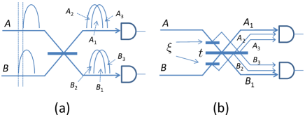
Figure 1: (a) Temporal mode mismatch at the beam splitter, and (b) its model based on effective beam splitters. $A_{i}$ and $B_{i}$ represent the modes where $A$ and $B$ corresponds to the spatial mode and the subscript are the labels for the temporal modes. Note that our model in (b) is phenomenological and thus is not restricted to the temporal mode mismatch.

Mode mismatch. Imperfection of mode matching at a beam splitter degrades the interference visibility. Let $\xi$ be a phenomenological mode match factor representing the overlap between two pulses, i.e. $0\leq\xi\leq 1$ where $\xi=1$ corresponds to a perfect mode matching while $\xi=0$ means the two pulses are in completely different modes and there is no interference between them. Then the effect of mode mismatch is modeled by adding two (effective) beam splitters with transmittance $\xi$. Figure 1(a) and (b) depict an example of the mode mismatch between two single-mode pulses in temporal mode and its translation into the beam splitting model (spatial mode), respectively, where the two pulses are partially overlapped. In spatial mode $A$ of Fig. 1(a), one can choose a temporal mode expansion in which one of the orthonormal mode is fully occupied by the pulse (i.e. includes $A_{1}$ and $A_{3}$). At the beam splitter, the mode expansion should be transformed such that the temporal part $A_{1}$ and $A_{3}$ are separated where these two modes should be a mixture with vacua to fulfil the normalization condition. This mode transformation is mathematically equivalent to split the pulse via a (virtual) beam splitter with transmittance $\xi$ into two spatial modes $A_{1}$ and $A_{3}$ (and combined it with a vacuum from the other port of the beam splitter). The same thing happens in spatial mode $B$ where the pulse is split into modes $B_{1}$ and $B_{2}$. Then $A_{i}$ and $B_{i}$ are combined at the real beam splitter where the pulses are interfered only between $A_{1}$ and $B_{1}$ (Fig. 1(b)).

Here we give an example. Suppose we would like to measure the coincidence counts after interfering the two Gaussian state pulses via a beam splitter with transmittance $t$. Let $\gamma_{A_{1}B_{1}}$ be the covariance matrix of the two-mode state (i.e. two pulses) before the beam splitter. Then after the beam splitting, a whole state is described by a six-mode covariance matrix

$$\tilde{\gamma}_{A_{1}B_{1}A_{2}B_{2}A_{3}B_{3}}=$$

$$S^{T}_{\rm BS}S^{T}_{\rm MM}(\gamma_{A_{1}B_{1}}\otimes I_{A_{2}B_{2}A_{3}B_{3}})S_{\rm MM}S_{\rm BS},$$ (21)

where

$$S_{\rm MM} = S^{\xi}_{B_{1}B_{3}}S^{\xi}_{A_{1}A_{2}},$$ (22)

$$S_{\rm BS} = S^{t}_{A_{3}B_{3}}S^{t}_{A_{2}B_{2}}S^{t}_{A_{1}B_{1}},$$ (23)

and the terms in the rhs are the beam splitter matrices defined in Eq. (14).

The coincidence count probability is then given by

$${\rm Tr}[\rho^{\tilde{\gamma}}(\hat{I}-|0\rangle\langle 0|^{\otimes 3})_{A_{1}A_{2}A_{3}}(\hat{I}-|0\rangle\langle 0|^{\otimes 3})_{B_{1}B_{2}B_{3}}].$$

Note that in our model, the mode mismatch is included by a phenomenological factor and thus we can incorporate any kinds of mode mismatch, such as temporal, spectral, spatial, etc.

II.6 Feedforward

Before closing the section, we briefly mention the (classical) feedforward operations. Feedforward is an important resource in QIP. For example, it allows one to implement an on-demand single-photon source from heralding of the SPDC photons Migdall2002 , and even constructing a universal quantum computer Knill2001 ; Prevedel2007 . In the feedforward scenario, each operation in the system can be adaptively chosen according to the prior partial measurement outcomes. Therefore, to fully simulate such a system, one has to calculate all possible branches of the measurement outcomes and feedforwarded operations. As will be discussed in section 3.3, since the computational complexity of our method exponentially grows as the system size increases, with our method it is not possible to fully simulate a large scale linear optics quantum computer proposed in Knill2001 with an efficient computation time. Note however, for relatively small size systems, it is possible to trace each feedforward branches and apply our method to calculate the probability of observing each event separately. That would be useful to simulate the currently (or near future) feasible experimental setups such as Migdall2002 ; Prevedel2007 .

III Applications

In this section we apply our characteristic function approach to SPDC based QIPs and compare some of them with previous experimental results.

III.1 Hong-Ou-Mandel interference of an SPDC source

The Hong-Ou-Mandel (HOM) interference is observed when two indistinguishable single-photons are interfered via a 50/50 beam splitter Hong1987 . The visibility of the HOM interference can be unit only when the two photons are fully indistinguishable in any degree of freedom (temporal mode, frequency mode, etc) which is thus a useful measure to evaluate the indistinguishability of the signal and idler photons from the same SPDC source. The HOM interference test for an SPDC source is described as follows. The signal and idler pulses are interfered by a 50/50 beam splitter and the coincidence count of the two detectors are measured by scanning the time delay of the idler pulse. The HOM dip is observed when there is no time delay for the idler pulse, i.e, the overlap of the signal and the idler in time is maximum. Let $P^{CC}_{\rm min}$ be the coincidence count (CC) probability without the delay and $P^{CC}_{\rm mean}$ be the CC probability with the delay which is enough larger than the pulse width such that no interference occurs between the signal and idler pulses. Following the previous works e.g. Sekatski2012 ; Jin2014SR , we define the visibility of the HOM test by

$$V_{\rm HOM}=\frac{P^{CC}_{\rm mean}-P^{CC}_{\rm min}}{P^{CC}_{\rm mean}}.$$ (24)

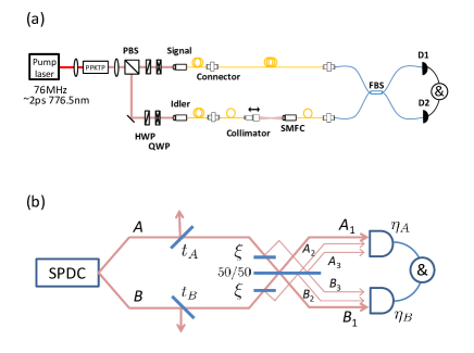
Figure 2: (a) Experimental setup of the HOM experiment in Jin2014SR , and (b) the corresponding linear optics model. PPKTP: periodically poled KTiOPO₄. PBS: polarization beam splitter. HWP: half waveplate. QWP: quarter waveplate. SMFC: single-mode fiber coupler. FBS: fiber beam splitter.

To see the validity of our method, we simulate the HOM experiment in Jin2014SR where the pump power dependence of $V_{\rm HOM}$ is experimentally observed with a standard mode-locked laser (Ti:Sapphire laser with a repetition rate of 76MHz). The experimental setup and the corresponding theoretical model are shown in Fig. 2(a) and (b), respectively.

The output from the SPDC source is described by a TMSV which fully includes the multi-photon components. The transmission losses in the signal ($A$) and idler modes ($B$), that are for example caused by coupling the spatial modes into fibers, are described by beam splitters with the transmittance $t_{A,B}$, respectively. Also $t_{B}$ includes the losses in the controllable delay line (the collimator in Fig. 2(a)) which makes the setup asymmetric (in the sense that $t_{A}\neq t_{B}$). $\eta_{A}$ and $\eta_{B}$ are the quantum efficiencies of the two photon detectors. The mode mismatch between the signal and idler pulses at the 50/50 beam splitter is characterized by the mode match factor $\xi$ which is in fact very sensitive to the HOM interference visibility as shown below.

The covariance matrix of the state generated from the SPDC is given by $\gamma_{AB}^{\rm TMSV}(\mu)$ which is defined in Eq. (8). Applying losses in mode $A$ and $B$ with transmittance $t_{A}$ and $t_{B}$, respectively, we get

$$\gamma^{\mathcal{L}}_{AB} = \mathcal{L}_{B}^{t_{B}}\mathcal{L}_{A}^{t_{A}}\gamma_{AB}^{\rm TMSV}(\mu)$$ (27)

$$= K_{AB}^{t_{A}t_{B}\,T}\gamma_{AB}^{\rm TMSV}(\mu)K_{AB}^{t_{A}t_{B}}+\alpha_{AB}^{t_{A}t_{B}}$$

$$= \left[\begin{array}[]{cc}2t_{A}\mu+1&\pm 2\sqrt{t_{A}t_{B}\mu(\mu+1)}\\ \pm 2\sqrt{t_{A}t_{B}\mu(\mu+1)}&2t_{B}\mu+1\end{array}\right]^{\oplus 2},$$

where

$$K_{AB}^{t_{A}t_{B}}=\left[\begin{array}[]{cc}\sqrt{t_{A}}&0\\ 0&\sqrt{t_{B}}\end{array}\right]^{\oplus 2},$$ (29)

and

$$\alpha_{AB}^{t_{A}t_{B}}=\left[\begin{array}[]{cc}1-t_{A}&0\\ 0&1-t_{B}\end{array}\right]^{\oplus 2}.$$ (30)

Application of a 50/50 beam splitter with mode matching factor $\xi$ is calculated to be

$$\gamma^{\rm BS}_{A_{1}A_{2}A_{3}B_{1}B_{2}B_{3}}$$

$$=S^{T}_{\rm BS}S^{T}_{\rm MM}(\gamma^{\mathcal{L}}_{A_{1}B_{1}}\oplus I_{A_{2}B_{2}A_{3}B_{3}})S_{\rm MM}S_{\rm BS},$$ (31)

where $S_{\rm MM}$ and $S_{\rm BS}$ are given by Eqs. (22) and (23) with $t=1/2$, respectively. $I_{A_{2}B_{2}A_{3}B_{3}}$ is a 8-by-8 identity matrix representing the vacua in modes $A_{2}$, $B_{2}$, $A_{3}$, and $B_{3}$. Finally photon detection consists of lossy channels corresponding to the detector loss and perfect detectors. The covariance matrix of the system after the lossy channels with $\eta_{A}$ and $\eta_{B}$, corresponding to the quantum efficiencies of two detectors, are given by

$$\gamma_{A_{1}\dots B_{3}}=\mathcal{L}_{B_{1}B_{2}B_{3}}^{\eta_{B}}\mathcal{L}_{A_{1}A_{2}A_{3}}^{\eta_{A}}\gamma^{\rm BS}_{A_{1}\dots B_{3}}.$$ (32)

We are now at the position to derive the coincidence count probability:

$$P^{CC}_{\rm min} = {\rm Tr}\left[\hat{\rho}^{\gamma_{A_{1}\dots B_{3}}}\left(\hat{I}-|0\rangle\langle 0|^{\otimes 3}\right)_{A_{1}A_{2}A_{3}}\left(\hat{I}-|0\rangle\langle 0|^{\otimes 3}\right)_{B_{1}B_{2}B_{3}}\right]$$ (33)

$$= 1-{\rm Tr}\left[\hat{\rho}^{\gamma_{A_{1}A_{2}A_{3}}}|0\rangle\langle 0|^{\otimes 3}_{A_{1}A_{2}A_{3}}\right]-{\rm Tr}\left[\hat{\rho}^{\gamma_{B_{1}B_{2}B_{3}}}|0\rangle\langle 0|^{\otimes 3}_{B_{1}B_{2}B_{3}}\right]+{\rm Tr}\left[\hat{\rho}^{\gamma_{A_{1}\dots B_{3}}}|0\rangle\langle 0|^{\otimes 6}_{A_{1}\dots B_{3}}\right]$$

$$= 1-\frac{8}{\sqrt{{\rm det}(\gamma_{A_{1}A_{2}A_{3}}+I)}}-\frac{8}{\sqrt{{\rm det}(\gamma_{B_{1}B_{2}B_{3}}+I)}}+\frac{64}{\sqrt{{\rm det}(\gamma_{A_{1}\dots B_{3}}+I)}},$$

where $\gamma_{A_{1}A_{2}A_{3}}$ and $\gamma_{B_{1}B_{2}B_{3}}$ are the submatrices of $\gamma_{A_{1}\dots B_{3}}$. The determinants in Eq. (33) are explicitly given by

$$\sqrt{{\rm det}(\gamma_{A_{1}A_{2}A_{3}}+I)} = 8\left\{\left[1+\frac{\eta_{A}\mu}{4}\left\{2(t_{A}+t_{B})-t_{A}t_{B}\eta_{A}(1-\xi^{2})\right\}\right]^{2}-t_{A}t_{B}\eta_{A}^{2}\xi^{2}\mu(\mu+1)\right\}^{1/2},$$ (34)

$$\sqrt{{\rm det}(\gamma_{B_{1}B_{2}B_{3}}+I)} = 8\left\{\left[1+\frac{\eta_{B}\mu}{4}\left\{2(t_{A}+t_{B})-t_{A}t_{B}\eta_{B}(1-\xi^{2})\right\}\right]^{2}-t_{A}t_{B}\eta_{B}^{2}\xi^{2}\mu(\mu+1)\right\}^{1/2},$$ (35)

$$\sqrt{{\rm det}(\gamma_{A_{1}\dots B_{3}}+I)} = 64\left[\left\{1+\frac{\mu}{4}\left[2(t_{A}+t_{B})(\eta_{A}+\eta_{B})-t_{A}t_{B}\left\{(\eta_{A}+\eta_{B})^{2}-\xi^{2}(\eta_{A}-\eta_{B})^{2}\right\}\right]\right\}^{2}\right.$$ (36)

$$\left.-t_{A}t_{B}(\eta_{A}-\eta_{B})^{2}\xi^{2}\mu(\mu+1)\right]^{1/2}.$$

The coincidence count with delay, $P^{CC}_{\rm mean}$ is simply obtained from $P^{CC}_{\rm min}$ by setting $\xi=0$, i.e. no overlap between the two modes.

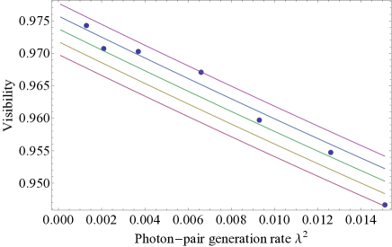
Figure 3: The experimental plots with the 76 MHz laser in Jin2014SR and the theoretical curves of the HOM visibility as a function of $\lambda^{2}$. The theoretical curves are with $\xi=$0.9888, 0.9878, 0.9868, 0.9858, and 0.9849 from the top to the bottom.

The theoretical visibilities derived above and the experimental plots in Jin2014SR are compared in Fig. 3 where the two channel transmittances were experimentally measured as $t_{A}=0.42$, $t_{B}=0.29$. The detectors used in the experiment were superconducting nanowire single photon detectors (SNSPDs) that gave $\eta_{A}=0.68$, and $\eta_{B}=0.70$ and negligible dark counts (less than 1k counts per second). The squeezing parameter $\lambda^{2}$ corresponds to the photon-pair generation rate which is directly measurable in the experiment (recall that $\lambda^{2}=\mu/(1+\mu)$). The mode matching factor is not measured and thus given as a fitting parameter. The figure shows a quantitative agreement between the theory and the experiment. Also the theory curves reveal that the visibility is highly sensitive to the mode matching at the beam splitter. Note that Jin2014SR also provides the theoretical curves, that are obtained by directly calculating the state vector of a whole system including environments and numerically computed the coincidence counts. One can numerically check that the numerical result in Jin2014SR and the theoretical curve in Fig. 3 are exactly identical. However, our method is much simpler and more systematic than the approach in Jin2014SR and allows us to obtain a closed formula. From that closed formula, we can also derive a simple analytical picture of the visibility. Suppose experimental imperfection is only the low efficiency of the detectors $\eta_{A}=\eta_{B}=\eta\ll 1$ and $t_{A}=t_{B}=\xi=1$. Assuming $\mu\ll 1$, which is reasonable for the photon-pair experiments, the visibility is simply given by

$$V_{\rm HOM}\approx\frac{1+2\mu}{1+4\mu}\approx 1-2\mu.$$ (37)

It should be noted that Eq. (37) agrees with the one obtained in Sekatski2012 . Another interesting limit is the ideal case ($t_{A}=t_{B}=\eta_{A}=\eta_{B}=\xi=1$ and $\mu\ll 1$):

$$V_{\rm HOM}\approx\frac{2+2\mu}{2+3\mu}\approx 1-\frac{1}{2}\mu,$$ (38)

which shows that the visibility degradation due to the multi-photon emission is accelerated by the low efficiency of the detectors.

III.2 EPR interference of a Sagnac loop entanglement source

Another example is the EPR interference test (also called correlation measurement) for polarization entangled photon pairs. We consider the Sagnac loop entanglement source, which was proposed in Shi2004 and is now widely used for photonic QIP experiments Jin2014OE ; Kim2006 ; Fedrizzi2007 ; Prevedel2011 ; Jin2014swap . Here we compare our model with the EPR interference experiment performed by a Sagnac loop entanglement source in Jin2014OE . The experimental set up and the corresponding theoretical model are illustrated in Figs. 4(a) and (b), respectively.

The Sagnac loop source generates a TMSV into the horizontal and vertical polarization modes in the clockwise direction (labeled as $A_{H},A_{V}$ in the theoretical model) and the counter-clockwise direction ($B_{H},B_{V}$). The entangled state is generated by swapping the vertical polarization modes $A_{V}$ and $B_{V}$ via a dichroic polarization beam splitter (DPBS). This operation transforms the covariance matrix of the two TMSV states $\gamma_{A_{H}A_{V}B_{H}B_{V}}^{\rm TMSV2}$ into $\gamma_{A_{H}A_{V}B_{H}B_{V}}^{\rm SL}$ where

$$\gamma_{A_{H}A_{V}B_{H}B_{V}}^{\rm TMSV2} = \left[\begin{array}[]{cccc}2\mu+1&\pm 2\sqrt{\mu(\mu+1)}&0&0\\ \pm 2\sqrt{\mu(\mu+1)}&2\mu+1&0&0\\ 0&0&2\mu+1&\pm 2\sqrt{\mu(\mu+1)}\\ 0&0&\pm 2\sqrt{\mu(\mu+1)}&2\mu+1\end{array}\right]^{\oplus 2},$$ (43)

$$\gamma_{A_{H}A_{V}B_{H}B_{V}}^{\rm SL} = \left[\begin{array}[]{cccc}2\mu+1&0&0&\pm 2\sqrt{\mu(\mu+1)}\\ 0&2\mu+1&\pm 2\sqrt{\mu(\mu+1)}&0\\ 0&\pm 2\sqrt{\mu(\mu+1)}&2\mu+1&0\\ \pm 2\sqrt{\mu(\mu+1)}&0&0&2\mu+1\end{array}\right]^{\oplus 2}.$$ (48)

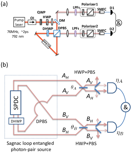
Figure 4: (a) Experimental setup of the EPR interference experiment in Jin2014OE , and (b) the corresponding linear optics model. PPKTP: periodically poled KTiOPO₄. OI: optical isolator. HWP: half waveplate. QWP: quarter waveplate. DM: dichroic mirror. DPBS: dichroic polarization beam splitter. DHWP: dichroic half waveplate. LPF: long wavelength pass filter. SMFC: single-mode fiber coupler.

The EPR interference test is a common and relatively easy way to experimentally estimate the quality of entanglement. Each spatial mode is projected onto a particular polarization basis by a half-wave plate (HWP) and a polarization beam splitter (PBS) and then the photons in a chosen polarization are detected by a single photon detector. The coincidence photon count rate depends on the angle of each polarization basis and the interference fringe is obtained by fixing one of the polarization angles constant and rotate the other one. The visibility is given by

$$V_{\rm ent}=\frac{P^{CC}_{\rm max}-P^{CC}_{\rm min}}{P^{CC}_{\rm max}+P^{CC}_{\rm min}},$$ (49)

where $P^{CC}_{\rm max}$ and $P^{CC}_{\rm min}$ are the maximum and minimum count rates in the fringe.

The polarizer (HWP and PBS) with angle $\theta$ effectively works as a beam splitter between the horizontal and vertical polarization modes with transmittance $\cos^{2}\theta$. The main imperfection in this component is a finite extinction ratio in the PBS which is modeled by a perfect beam splitter followed by losses in each polarization mode with $t_{H}<1$ and $t_{V}>0$ where $t_{H}$ and $t_{V}$ are the transmittances of the horizontal and vertical polarization modes, respectively (see Fig. 5(a) and (b)). In the following, to simplify the calculation of the setup in Fig. 4(b), we use $\tilde{\eta}_{H}=t_{H}\eta_{H}$ and $\tilde{\eta}_{V}=t_{V}\eta_{V}$ where $\eta_{H}$ and $\eta_{V}$ are the quantum efficiencies of the detector for horizontally and vertically polarized photons, respectively. The covariance matrix of the entangled source in Eq. (48) is first transformed by perfect beam splitter operations $S^{\theta_{B}}_{B_{H}B_{V}}S^{\theta_{A}}_{A_{H}A_{V}}$. The imperfection of the PBSs and the imperfect quantum efficiency of the detectors are included by applying the lossy channels $\mathcal{L}_{B_{V}}^{\tilde{\eta}_{B_{V}}}\mathcal{L}_{B_{H}}^{\tilde{\eta}_{B_{H}}}\mathcal{L}_{A_{V}}^{\tilde{\eta}_{A_{V}}}\mathcal{L}_{A_{H}}^{\tilde{\eta}_{A_{H}}}$. The coincidence count is then given by

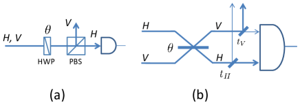
Figure 5: (a) The polarizer consisting of a half waveplate (HWP) and a polarization beam splitter (PBS), and (b) the corresponding linear optics model.

$$P^{CC}_{\theta_{A}\theta_{B}} = {\rm Tr}\left[\hat{\rho}^{\gamma_{A_{H}A_{V}B_{H}B_{V}}}\left(\hat{I}-|0\rangle\langle 0|^{\otimes 2}\right)_{A_{H}A_{V}}\left(\hat{I}-|0\rangle\langle 0|^{\otimes 2}\right)_{B_{H}B_{V}}\right]$$ (50)

$$= 1-\frac{4}{\sqrt{{\rm det}(\gamma_{A_{H}A_{V}}+I)}}-\frac{4}{\sqrt{{\rm det}(\gamma_{B_{H}B_{V}}+I)}}+\frac{16}{\sqrt{{\rm det}(\gamma_{A_{H}A_{V}B_{H}B_{V}}+I)}},$$

where

$$\sqrt{{\rm det}(\gamma_{A_{H}A_{V}}+I)} = 4(1+\tilde{\eta}_{A_{H}}\mu)(1+\tilde{\eta}_{A_{V}}\mu),$$ (51)

$$\sqrt{{\rm det}(\gamma_{B_{H}B_{V}}+I)} = 4(1+\tilde{\eta}_{B_{H}}\mu)(1+\tilde{\eta}_{B_{V}}\mu),$$ (52)

$$\sqrt{{\rm det}(\gamma_{A_{H}A_{V}B_{H}B_{V}}+I)} = 8\left[\left\{1+(\tilde{\eta}_{A_{H}}+\tilde{\eta}_{B_{H}}-\tilde{\eta}_{A_{H}}\tilde{\eta}_{B_{H}})\mu\right\}\left\{1+(\tilde{\eta}_{A_{V}}+\tilde{\eta}_{B_{V}}-\tilde{\eta}_{A_{V}}\tilde{\eta}_{B_{V}})\mu\right\}\right.$$ (53)

$$\left.+\left\{1+(\tilde{\eta}_{A_{H}}+\tilde{\eta}_{B_{V}}-\tilde{\eta}_{A_{H}}\tilde{\eta}_{B_{V}})\mu\right\}\left\{1+(\tilde{\eta}_{A_{V}}+\tilde{\eta}_{B_{H}}-\tilde{\eta}_{A_{V}}\tilde{\eta}_{B_{H}})\mu\right\}\right.$$

$$\left.+(\tilde{\eta}_{A_{H}}-\tilde{\eta}_{A_{V}})(\tilde{\eta}_{B_{H}}-\tilde{\eta}_{B_{V}})\mu(\mu+1)\cos 2(\theta_{A}+\theta_{B})\right].$$

The minimum and maximum count rates required in Eq. (49) are for example obtained by $P^{CC}_{\rm min}=P^{CC}_{0\,0}$ and $P^{CC}_{\rm max}=P^{CC}_{0\,\pi/2}$ Jin2014OE .

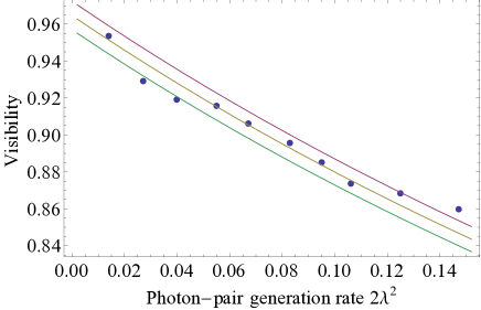
Figure 6: The experimental plots in Jin2014OE and the theoretical curves of the EPR interference as a function of the photon-pair generation rate of the Sagnac loop source $2\lambda^{2}$. The theoretical curves are with $t_{V}=$0.007, 0.009, and 0.011 from the top to the bottom.

Figure 6 shows the comparison with the experiment in Jin2014OE and our theoretical model. Note that the photon-pair generation rate of the Sagnac loop source should be $2\lambda^{2}$ instead of $\lambda^{2}$ since the SPDC crystal is pumped twice (clockwise and counter-clockwise directions). In the experiment, the overall efficiencies for the horizontal polarization are measured to be $\tilde{\eta}_{A_{H}}=\tilde{\eta}_{B_{H}}=0.1$ (again, SNSPDs are used as detectors and thus we neglect the effect of dark counts). The transmittance of the vertical polarization at the PBS is not measured and thus we use it as a fitting parameter varying from 0.007 to 0.011 ($\leq 0.01$ is guaranteed for a typical commercial PBS). The theoretical estimate agrees with the experimental result.

Again, it is worth to further simplify the closed form given above. By setting $\tilde{\eta}_{A_{V}}=\tilde{\eta}_{B_{V}}=0$ and $\tilde{\eta}_{A_{H}}=\tilde{\eta}_{B_{H}}=\eta$, the closed form of the visibility is reduced to

$$V_{\rm ent}=\frac{1+\mu}{1+3\mu+2\eta(2-\eta)\mu^{2}}.$$ (54)

In the limit of weak pumping ($\mu\ll 1$), we have

$$V_{\rm ent}\approx 1-2\mu,$$ (55)

regardless of the detection efficiency $\eta$. Those results agree with the previous analyses in Kuzucu2008 ; Takesue2010 ; Sekatski2012 . .

III.3 Concatenated entanglement swapping

The last application in this section is the concatenated entanglement swapping (CES) where we show how to apply our method to the QIP protocols with a multiple use of entangled source and demonstrate a drastic improvement of the computation time compared to the previous approach. Entanglement transmission over long distance is limited by the loss and noises in channel and detectors. Quantum repeater can overcome this limit but it is still challenging to implement it in large scale with the current technology. Concatenation of entanglement swapping (also called quantum relay) is known as another protocol to extend the distance of the entanglement distribution albeit with a resource overhead that is exponential in the distance (which is usually observed as an exponential decrease of the success probability) Gisin2002 . However, since entanglement swapping has been demonstrated with the current technology (see Jin2014swap and references therein), it is still interesting to see the practical performance of the CES protocol in theory.

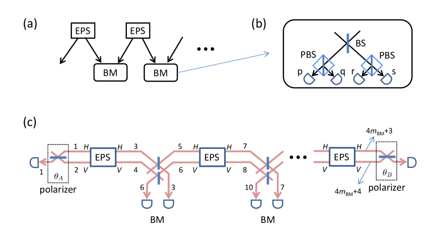
Figure 7: (a) Schematic of the concatenated entanglement swapping and (b) the Bell measurement for polarized entangled photons. (c) Corresponding linear optics model (see the text for details). EPS: entangled photon source. BM: Bell measurement. BS: beam splitter. PBS: polarizing beam splitter. $m_{\rm BM}$: number of the Bell measurements used in the CES protocol.

The protocol considered here is similar to the CES model discussed in detail in Khalique2013 where the state vector evolution of the two-mode squeezed state generated from SPDCs are calculated and the authors showed explicit expression of the density matrix and the detection probabilities those are used to derive the visibility of the EPR interference of the distributed entanglement numerically. Figure 7(a) illustrates the schematic of the protocol. Entangled photon-pairs generated from the entangled photon-pair sources (EPSs) are swapped by the Bell measurement consisting of a 50/50 beam splitter, two PBSs and four on-off type photon detectors (Fig. 7(b)). Entanglement swapping succeeds when photons are detected by particular two detectors in the Bell measurement for example at q and s in Fig. 7(b). For more details of the protocol see Khalique2013 and the references therein.

Figure 7(c) is our model which is equivalent to Fig. 7(a) but the orthogonal polarization modes are explicitly illustrated by different lines. For our EPS, we assume to use the Sagnac loop SPDC entangled source discussed in the previous subsection while the method can be applied to any other sources even not necessarily entangled in polarization modes (such as time-bin entanglements). For the system imperfections, we follow the assumptions used in Khalique2013 , i.e. losses in channels and detectors and the dark counts at detectors exist whereas the mode matching at beam splitters and the PBS devices are assumed to be perfect. The polarization modes are labeled by numbers from the left to the right (see Fig. 7(c)). Also in the figure, for simplicity, only two detectors are illustrated for each Bell measurement where the simultaneous clicks at these detectors correspond to the successful CES. At the left and right ends, two polarizers (see Fig. 5) are placed to measure the EPR interference visibility of the swapped state.

We now calculate the joint detection probability of all detectors illustrated in Fig. 7(c) as a function of two polarizer angles $\theta_{A}$ and $\theta_{B}$. Let $m_{\rm BM}$ be the number of Bell measurements (the number of concatenation), i.e. there are $m_{\rm BM}+1$ Sagnac loop sources (EPSs). The covariance matrix for the quantum state generated from the most left Sagnac loop SPDC is $\gamma^{\rm SL}_{1234}$ as discussed in Eq. (48). The total quantum state generated from $m_{\rm BM}+1$ Sagnac loops is thus simply given by $\gamma^{\rm SL\,\oplus(m_{\rm BM}+1)}$, more precisely,

$$\left[\begin{array}[]{ccc}\gamma^{\rm SL}_{\pm}(\mu)&0&\cdots\\ 0&\gamma^{\rm SL}_{\pm}(\mu)&\\ \vdots&&\ddots\end{array}\right]^{\oplus 2},$$ (56)

where $\gamma^{\rm SL}\equiv\left(\gamma^{\rm SL}_{\pm}(\mu)\right)^{\oplus 2}$ and thus $\gamma^{\rm SL}_{\pm}(\mu)$ correspond to the two quadrature components of $\gamma^{\rm SL}$. Following the discussion in Scherer2009 ; Khalique2013 , all transmission loss is included in the detector efficiency. We also assume that all transmission channels have the same loss and all detectors are identical. Therefore, we first apply the beam splitting operations at the Bell measurements. The beam splitters combine modes $4x-1$ and $4x+1$ for horizontal polarizations and modes $4x$ and $4x+2$ for vertical polarizations where $x=1,\dots,m_{\rm BM}$. Thus the symplectic matrix applied to $\gamma^{\rm SL\,\oplus(m_{\rm BM}+1)}$ is

$$S_{\rm BM}=\prod_{x=1}^{m_{\rm BM}}S^{1/2}_{4x-1,4x+1}S^{1/2}_{4x,4x+2}.$$ (57)

The two polarizer operations at the end of the concatenation are also given by applying the beam splitter symplectic matrix

$$S_{\rm AB}=S^{\theta_{A}}_{1,2}S^{\theta_{B}}_{4m_{\rm BM}+3,4m_{\rm BM}+4}.$$ (58)

Let $\eta$ be the detector efficiency (including the channel transmittance). This is included by applying

$$\mathcal{L}^{\eta}_{\rm tot}=\mathcal{L}^{\eta}_{4m_{\rm BM}+4}\cdots\mathcal{L}^{\eta}_{1},$$ (59)

to the covariance matrix of the state. In total, we have the covariance matrix

$$\gamma^{CES}_{m_{\rm BM}}=\mathcal{L^{\eta}_{\rm tot}}\left(S_{\rm AB}^{T}S_{\rm BM}^{T}\gamma^{\rm SL\,\oplus(m_{\rm BM}+1)}S_{\rm BM}S_{\rm AB}\right).$$ (60)

The joint detection probability of all detectors illustrated in Fig. 7(c) is now obtained by calculating

$$P^{CES}_{\theta_{A}\theta_{B}} = {\rm Tr}\left[\hat{\rho}^{\gamma^{CES}_{m_{\rm BM}}}\left(\hat{I}-(1-\nu)|0\rangle\langle 0|\right)_{1}\left(\hat{I}-(1-\nu)|0\rangle\langle 0|\right)_{4m_{\rm BM}+3}\prod_{x=1}^{m_{\rm BM}}\left(\hat{I}-(1-\nu)|0\rangle\langle 0|\right)_{4x-1}\left(\hat{I}-(1-\nu)|0\rangle\langle 0|\right)_{4x+2}\right]$$ (61)

$$= 1+\sum_{m=1}^{M}\sum_{C(M,m)}^{{}_{M}C_{m}}\frac{\{-2(1-\nu)\}^{m}}{\sqrt{{\rm det}(\gamma^{\rm CES}_{C(M,m)}+I)}},$$

where $\nu$ is the dark count rate of detectors, $M$ is the total number of clicked detectors, i.e. $M=2m_{\rm BM}+2$, and $\gamma^{\rm CES}_{C(M,m)}$ is the submatrix of $\gamma^{\rm CES}$ taking only modes $C(M,m)$. $C(M,m)$ is the $m$-detector combination from $M$ detectors. For example, when $m_{\rm BM}=1$, total number of detectors is $M=4$ and the detectors are placed in modes 1, 3, 6, and 7. Then $C(4,1)=$1, 3, 6, 7, $C(4,2)=$13, 16, 17, 36, 37, 67, $C(4,3)=$136, 137, 167, 367, and $C(4,4)=$1367. For reference, we describe a detailed structure of $\gamma^{CES}_{\rm m_{\rm BM}}$ in Appendix.

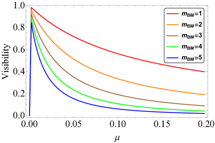
Figure 8: The EPR interference visibility of the entangled state distributed by the concatenated entanglement swapping as a function of the squeezing parameter $\mu$ with $\eta=0.04$ and $\nu=10^{-5}$ (see the main text). The number of the Bell measurements (concatenation) is $m_{\rm BM}=$1, 2, 3, 4, and 5 for red, orange, brown, green, and blue lines.

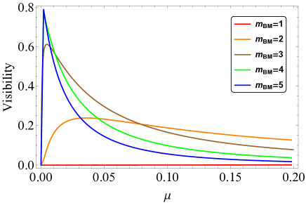
Figure 9: The EPR interference visibility for the same transmission distance with different number of concatenation. Transmittance of the whole channel is $10^{-20}$ which corresponds to 1000km distance by a standard fiber with loss of $0.2$dB/km. Efficiency and dark counts of the detectors are $\eta_{\rm D}=0.7$ and $\nu=10^{-5}$, respectively. The number of the Bell measurements (concatenation) is $m_{\rm BM}=$1, 2, 3, 4, and 5 for red, orange, brown, green, and blue lines.

In Fig. 8, the EPR interference visibilities are plotted as a function of $\mu$ for $m_{\rm BM}=1,\dots,5$. For comparison, we choose the parameters used in Khalique2013 , $\eta=0.04$ and $\nu=10^{-5}$ for the transmittance and dark counts, respectively. In Khalique2013 , the CES with $m_{\rm BM}=3$ is numerically simulated by a super computer with the photon number truncation at 3 photons in each mode (the authors also reported that it takes 6 hours to get a single plot for the same simulation by a single-core use of a commercially available computer). In Fig. 8, the curve for $m_{\rm BM}=3$ (brown line) consists of 400 plots that are calculated by a commercial computer with only 10 seconds without any photon number truncation. Similarly, 100 plots for $m_{\rm BM}=5$ (blue line) require around 2 minutes with the same computer (it should be noted that our method works only for on-off detectors while the mathematical formula in Khalique2013 includes both for on-off and photon number resolving detectors).

Our method is useful to estimate the performance of the CES for the long-distance entanglement transmission. In our model the total transmittance consists of the detector efficiency and the channel transmission as $\eta=\eta_{\rm D}\times 10^{-\alpha L/10}$ where $\eta_{\rm D}$ is the detector efficiency, $\alpha$ is the loss coefficient, and $L$ is the distance of the transmission channel. In the following, we consider the photon pairs at 1550 nm and use of a standard optical fiber with $\alpha=0.2$ as a transmission channel. Figure 9 compares the visibility for different $m_{\rm BM}$ where the total distance of the channel is fixed to be 1000 km. The detector efficiency and dark counts are assumed to be $\eta_{\rm D}=0.7$ and $\nu=10^{-5}$, respectively, could be typical parameters for SNSPDs discussed in previous subsections. For example, for $m_{\rm BM}=1$, the channel is divided into four arms and each arm has 250 km distance. In Fig. 9, the visibility is plotted for the CES up to $m_{\rm BM}=5$. First it shows that for $m_{\rm BM}=1$, it is completely impossible to distribute entanglement and even for $m_{\rm BM}=2$, the visibility must be around 0.2. Second, for extremely small $\mu$, the figure shows that $m_{\rm BM}$ should be large as much as possible while for the most region of $\mu$, the curve for $m_{\rm BM}=5$ decreases quickly as $\mu$ increases and $m_{\rm BM}=$3 or 4 are optimal for most of $\mu$. The result suggests that to construct a practical CES network, the optimal number of concatenation should be carefully chosen by considering a given distance (channel loss) and detector parameters.

Finally, it should be worth to mention about a general scaling of the computational complexity of our method with respect to the number of modes $N$ (or equivalently number of detectors to be detected). Our method is not efficient in the sense that the computational complexity grows exponential with respect to $N$. This is clearly observed in Eq. (61). There are two steps to compute Eq. (61). First, one has to calculate the covariance matrix including losses and beam splitters (in general any linear optics and even squeezing operations). This step consists of multiplications of square matrices and each of that is polynomial (at worst order of $O(N^{3})$ by direct calculation). Second, the determinants of the (sub)matrices in each term of Eq. (61) should be calculated. While determinants can be calculated for example with $O(N^{3})$ by the LU decomposition HornJohnson , the number of terms in the second line of Eq. (61) is increase as $2^{N}$ since the first line of Eq. (61) includes $N$ multiplication of binomial terms $(\hat{I}-(1-\nu)|0\rangle\langle 0|)$. This results the method inefficient (at least $O(2^{N})$ for simulating large scale networks. Note that this is not only for the CES protocols but a general property for any linear optics networks with SPDCs and photon detectors. However, we should stress that, as shown in this subsection, for experimentally feasible size of the network with the current technology or even larger sizes, our method can work as a powerful tool to estimate the performance of the protocols with a practical computational time.

IV Conclusion

In summary, we have proposed a method to compute the SPDC based QIP experiments theoretically, which fully involves the multi-photon emissions and various experimental imperfections. The key ingredient of our method is an application of the characteristic function formalism which has been widely used in CV-QIPs, in particular, for Gaussian states and operations. We apply our methods to three examples, the HOM interference and the EPR interference experiments, and the concatenated entanglement swapping protocol. The first two examples are compared with the previously reported experimental results and show quantitative agreements. Moreover, we provide the analytical expression for the HOM and EPR visibilities that include full multi-photon components and various experimental imperfections. These could be useful for estimating the performance of various experimental setups. In the third example, we numerically simulate the performance of the CES protocol up to five Bell measurements (concatenations) which requires only few minutes with a commercially available computer. Our method could be useful to estimate the practical performance of the SPDC based protocol with experimentally feasible or even larger size linear optics networks. Interesting future applications would include multi-partite entanglement generation Pan2012 , QKD Ekert1991 and quantum repeaters with SPDC sources such as heralded entanglements Barz2010 ; Usmani2012 .

Finally, a general computational complexity of our method with respect to the size of the system (mode numbers) is discussed. We show that the complexity is growing as $O(2^{N})$ and thus inefficient for simulating very large scale systems beyond the current or near-future technologies. In general, linear optics network with perfect single photons and photon number resolving detectors, it is impossible to efficiently simulate the large system classically which is why the linear optics with feedback can construct a universal quantum computer Knill2001 (related to this, it is believed that other related computing ideas such as Boson Sampling Aaronson2010 cannot be efficiently simulated by classical computers). Although we feel this would also be the case for linear optics system with SPDCs and on-off detectors, it remains as an important open question whether there exists an efficient algorithm to simulate such a system. We stress that, however, our method is at least applicable to simulate the proof-of-principle demonstration of these protocols Prevedel2007 ; Broome2013 ; Spring2013 ; Tillmann2013 ; Crespi2013 and also estimating even larger system that could be a real target in near-future experiments.

*

Appendix A The covariance matrix in the CES protocol

The explicit structure of $\gamma^{CES}(m_{\rm BM})$ in Eq. (60) is

$$\gamma^{CES}_{m_{\rm BM}}=\left[\begin{array}[]{cccccc}A_{2}&\pm B^{T}&0&0&0&0\\ \pm B&A_{4}&\pm C^{T}&0&0&0\\ 0&\pm C&A_{4}&\pm C^{T}&0&0\\ 0&0&\pm C&\ddots&\pm C^{T}&0\\ 0&0&0&\pm C&A_{4}&\pm D^{T}\\ 0&0&0&0&\pm D&A_{2}\end{array}\right]^{\oplus 2},$$ (62)

where

$$A_{2} = (2\eta\mu+1)I_{2},$$ (63)

$$A_{4} = \left[\begin{array}[]{cc}A_{2}&0\\ 0&A_{2}\end{array}\right],$$ (66)

$$B = \eta\sqrt{2\mu(\mu+1)}\left[\begin{array}[]{cc}\sin\theta_{A}&\cos\theta_{A}\\ \cos\theta_{A}&-\sin\theta_{A}\\ -\sin\theta_{A}&-\cos\theta_{A}\\ -\cos\theta_{A}&\sin\theta_{A}\end{array}\right],$$ (71)

$$C = \eta\sqrt{\mu(\mu+1)}\left[\begin{array}[]{cc}J_{2}&J_{2}\\ -J_{2}&-J_{2}\\ \end{array}\right],$$ (74)

$$D = \eta\sqrt{2\mu(\mu+1)}\left[\begin{array}[]{cccc}\sin\theta_{B}&\cos\theta_{B}&\sin\theta_{B}&\cos\theta_{B}\\ \cos\theta_{B}&-\sin\theta_{B}&\cos\theta_{B}&-\sin\theta_{B}\end{array}\right],$$ (77)

and

$$I_{2}=\left[\begin{array}[]{cc}1&0\\ 0&1\end{array}\right],\quad J_{2}=\left[\begin{array}[]{cc}0&1\\ 1&0\end{array}\right].$$ (79)

References

- (1) Jian-Wei Pan, Zeng-Bing Chen, Chao-Yang Lu, Harald Weinfurter, Anton Zeilinger, and Marek Żukowski . Multiphoton entanglement and interferometry. Review of Modern Physics, 84:777–838, 2012.
- (2) Onur Kuzucu and Franco N. C. Wong. Pulsed sagnac source of narrow-band polarization-entangled photons. Physical Review A, 77:032314–, 2008.
- (3) Roland Krischek, Witlef Wieczorek, Akira Ozawa, Nikolai Kiesel, Patrick Michelberger, Thomas Udem, and Harald Weinfurter. Ultraviolet enhancement cavity for ultrafast nonlinear optics and high-rate multiphoton entanglement experiments. Nature Photonics, 4:170–173, 2010.
- (4) Xiao-Song Ma, Stefan Zotter, Johannes Kofler, Thomas Jennewein, and Anton Zeilinger. Experimental generation of single photons via active multiplexing. Physical Review A, 83:043814, 2011.
- (5) M. A. Broome, M. P. Almeida, A. Fedrizzi, and A. G. White. Reducing multi-photon rates in pulsed down-conversion by temporal multiplexing. Optics Express, 19:22698, 2011.
- (6) Rui-Bo Jin, Ryosuke Shimizu, Isao Morohashi, Kentaro Wakui, Masahiro Takeoka, Shuro Izumi, Takahide Sakamoto, Mikio Fujiwara, Taro Yamashita, Shigehito Miki, Hirotaka Terai, Zhen Wang, and Masahide Sasaki. Efficient generation of twin photons at telecom wavelengths with 2.5 GHz repetition-rate-tunable comb laser. Scientific Reports, 4:7468, 2014.
- (7) Z. Y. Ou, J.-K. Rhee, and L. J. Wang. Photon bunching and multiphoton interference in parametric down-conversion. Physical Review A, 60:593, 1999.
- (8) Hugues de Riedmatten, Valerio Scarani, Ivan Marcikic, Antonio Acín, Wolfgang Tittel, Hugo Zbinden, and Nicolas Gisin. Two independent photon paris versus four-photon entangled states in parametric down conversion. Journal of Modern Optics, 51:1637, 2004.
- (9) V. Scarani, H. de Riedmatten, I. Marcikic, H. Zbinden, and N. Gisin. Four-photon correction in two-photon Bell experiments. The European Physical Journal D, 32:129, 2005.
- (10) Artur Scherer, Regina B. Howard, Barry C. Sanders, and Wolfgang Tittel. Quantum states prepared by realistic entanglement swapping. Physical Review A, 80:062310, 2009.
- (11) Witlef Wieczorek, Nikolai Kiesel, Christian Schmid, and Harald Weinfurter. Multiqubit entanglement engineering via projective measurements. Physical Review A, 79:022311, 2009.
- (12) Hiroki Takesue and Kaoru Shimizu. Effects of multiple pairs on visibility measurements of entangled photons generated by spontaneous parametric processes. Optics Communications, 283:276, 2010.
- (13) Thomas Jennewein, Marco Barbieri, and Andrew G. White. Single-photon device requirements for operating linear optics quantum computing outside the post-selection basis. Journal of Modern Optics, 58:276, 2011.
- (14) P Sekatski, N Sangouard, F Bussières, C Clausen, N Gisin, and H Zbinden. Detector imperfections in photon-pair source characterization. Journal of Physics B: Atomic, Molecular and Optical Physics, 45:124016, 2012.
- (15) Aeysha Khalique, Wolfgang Tittel, and Barry C. Sanders. Practical long-distance quantum communication using concatenated entanglement swapping. Physical Review A, 88:022336, 2013.
- (16) S. M. Barnett and P. M. Radmore. Methods in Theoretical Quantum Optics. Oxford University Press, New York, 1997.
- (17) Samuel L. Braunstein and Peter van Loock. Quantum information with continuous variables. Review of Modern Physics, 77:513, 2005.
- (18) Rui-Bo Jin, Ryosuke Shimizu, Kentaro Wakui, Mikio Fujiwara, Taro Yamashita, Shigehito Miki, Hirotaka Terai, Zhen Wang, and Masahide Sasaki. Pulsed Sagnac polarization-entangled photon source with a PPKTP crystal at telecom wavelength. Optics Express, 22:11498, 2014.
- (19) Christian Weedbrook, Stefano Pirandola, Raúl García-Patrón, Nicolas J. Cerf, Timothy C. Ralph, Jeffrey H. Shapiro, and Seth Lloyd. Gaussian quantum information. Review of Modern Physics, 84:621, 2012.
- (20) Stephen D. Bartlett, Barry C. Sanders, Samuel L. Braunstein, and Kae Nemot. Efficient classical simulation of continuous variable quantum information processes. Physical Review Letters, 88:097904, 2002.
- (21) Saikat Guha, Hari Krovi, Christopher A. Fuchs, Zachary Dutton, Joshua A. Slater, Christoph Simon, and Wolfgang Tittel. Exact analysis of a practical quantum repeater architecture with noisy elements. arXiv:1404.7183.
- (22) Stefano Olivares and Matteo G A Paris. Squeezed fock state by inconclusive photon subtraction. Journal of Optics B: Quantum and Semiclassical Optics, 7:S616, 2005.
- (23) Masahiro Takeoka and Masahide Sasaki. Discrimination of the binary coherent signal: Gaussian-operation limit and simple non-gaussian near-optimal receivers. Physical Review A, 78:022320, 2008.
- (24) F Caruso, V Giovannetti, and S Holevo. One-mode bosonic gaussian channels: a full weak-degradability classification. New Journal of Physics, 8:310, 2006.
- (25) Stephen M. Barnett, Lee S. Phillips, and David T. Pegg. Imperfect photodetection as projection onto mixed states. Optics Communications, 158:45, 1998.
- (26) A. L. Migdall, D. Branning, and S. Castelletto. Tailoring single-photon and multiphoton probabilities of a single-photon on-demand source. Physical Review A, 66:053805, 2002.
- (27) E. Knill, R. Laflamme, and G. J. Milburn. A scheme for efficient quantum computation with linear optics. Nature 409:46, 2001.
- (28) C. K. Hong, Z. Y. Ou, and L. Mandel. Measurement of subpicosecond time intervals between two photons by interference. Physical Review Letters, 59:2044, 1987.
- (29) Bao-Sen Shi and Akihisa Tomita. Generation of a pulsed polarization entangled photon pair using a Sagnac interferometer. Physical Review A, 69:013803, 2004.
- (30) Taehyun Kim, Marco Fiorentino, and Franco N. C. Wong. Phase-stable source of polarization-entangled photons using a polarization sagnac interferometer. Physical Review A, 73:012316, 2006.
- (31) Alessandro Fedrizzi, Thomas Herbst, Andreas Poppe, Thomas Jennewein, and Anton Zeilinger. A wavelength-tunable fiber-coupled source of narrowband entangled photons. Optics Express, 15:15377, 2007.
- (32) Robert Prevedel, Deny R. Hamel, Roger Colbeck, Kent Fisher, and Kevin J. Resch. Experimental investigation of the uncertainty principle in the presence of quantum memory and its application to witnessing entanglement. Nature Physics, 7:757, 2011.
- (33) Rui-Bo Jin, Masahiro Takeoka, Utako Takagi, Ryosuke Shimizu, and Masahide Sasaki. Highly efficient entanglement swapping and teleportation at telecom wavelength. Scientific Reports, 5:9333, 2015.
- (34) Nicolas Gisin, Gregoire Ribordy, Wolfgang Tittel, and Hugo Zbinden. Quantum cryptography. Review of Modern Physics, 74:145, 2002.
- (35) Roger A. Horn and Charles R. Johnson. Matrix Analysis. Cambridge University Press, Cambridge, 1985.
- (36) Artur K. Ekert. Quantum cryptography based on bell’s theorem. Physical Review Letters, 67:661, 1991.
- (37) Stefanie Barz, Gunther Cronenberg, Anton Zeilinger, and Philip Walther. Heralded generation of entangled photon pairs. Nature Photonics, 4:553, 2010.
- (38) Imam Usmani, Christoph Clausen, Félix Bussières, Nicolas Sangouard, Mikael Afzelius, and Nicolas Gisin. Heralded quantum entanglement between two crystals. Nature Photonics, 6:234, 2012.
- (39) Scott Aaronson and Alex Arkhipov. The computational complexity of linear optics. arXiv:1011.3245.
- (40) Robert Prevedel, Philip Walther, Felix Tiefenbacher, Pascal Bohi, Rainer Kaltenbaek, Thomas Jennewein, and Anton Zeilinger. High-speed linear optics quantum computing using active feed-forward. Nature, 445:65, 2007.
- (41) Matthew A Broome, Alessandro Fedrizzi, Saleh Rahimi-keshari, Justin Dove, Scott Aaronson, Timothy C. Ralph, and Andrew G White. Photonic boson sampling in a tunable circuit. Science, 339:794, 2013.
- (42) Justin B Spring, Benjamin J Metcalf, Peter C Humphreys, W Steven Kolthammer, Xian-min Jin, Marco Barbieri, Animesh Datta, Nicholas Thomas-peter, Nathan K Langford, Dmytro Kundys, James C Gates, Brian J Smith, Peter G R Smith, and Ian A Walmsley. Boson sampling on a photonic chip. Science, 339:798, 2013.
- (43) Max Tillmann, Borivoje Dakić, René Heilmann, Stefan Nolte, Alexander Szameit, and Philip Walther. Experimental boson sampling. Nature Photonics, 7:540, 2013.
- (44) Andrea Crespi, Roberto Osellame, Roberta Ramponi, Daniel J. Brod, Ernesto F. Galvão, Nicolò Spagnolo, Chiara Vitelli, Enrico Maiorino, Paolo Mataloni, and Fabio Sciarrino. Integrated multimode interferometers with arbitrary designs for photonic boson sampling. Nature Photonics, 7:545, 2013.