Isobar configurations: $\Delta N$ correlations
versus the independent particle model

We present a comparative analysis of two models for the $A({\gamma,\,\pi N})B$ reaction, which take into account the isobar configurations in the ground state of the nuclei: the $\Delta N$ correlation model and the quasifree pion photoproduction model. The considered models differ in their descriptions of the nucleus states. The $\Delta N$ correlation model takes into account the dynamic correlations of the nucleon and isobar formed in the virtual transition $NN\to\Delta N$, and in the quasifree pion photoproduction model, isobars and nucleons in the nucleus are considered as independent constituents. The predictions of the models are considered for two reactions ¹⁶O$({\gamma,\,\pi^{+}p}){}^{15}$C and ¹⁶O$({\gamma,\,\pi^{-}p}){}^{15}$O. It is shown, that the two models predict the differential cross section significantly differing both in absolute values, and in the shape of the angular dependence. We compare the results of the $\Delta N$ correlation model for the $({\gamma,\,\pi N})$ and $({\gamma,\,\pi NN})$ reactions with the ¹⁶O$({\gamma,\,\pi^{-}p})$ reaction data measured at BNL. Our results give support to the $\Delta N$ correlation model.

1 Introduction

For a long time, the role played by nucleon resonances as components of the atomic nucleus was intensively studied both experimentally and theoretically [1, 2]. According to theoretical estimates, some of the nucleons in the nucleus, as a result of collisions, can experience excitation of the internal degrees of freedom and go with a probability of a few percent to a virtual isobar states [3, 4]. To describe such nuclear states, the wave function of the nucleus, including the nucleon configurations, is complemented by isobar configurations, in which one or more nucleons are in an excited states. Consideration of the isobar configurations in the ground state of the nuclei is important in explaining both the static properties of the nuclei and the nuclear reactions.

Nuclear reactions that cannot be explained within a model that assumes a single interaction of a projectile particle with bound nucleons of a nucleus are an efficient tool in experimentally studying isobar degrees of freedom in the ground states of nuclei. As an example, we can indicate $({\pi^{+},\,\pi^{-}p})$ reactions [5, 6], where the charged state of a scattered particle changes by $2e$, or $({p,\,p^{\prime}\,\pi^{+}p})$ [7] and $({\gamma,\,\pi^{-}n})$ reactions accompanied by the production of particles whose total electric charge is +2 or $-$1. Such experimental data are usually interpreted, using the model of the quasifree knockout of the isobar [5, 6, 7, 8, 9]. The weakest element of this approach is the independent particle model, used as a model of the nucleus. Because the virtual isobar is formed in the nucleus owing to the $NN\to\Delta N$ and $NN\to\Delta\Delta$ transitions, the states of the nucleon and isobar of the $\Delta N$ system or the states of two isobars of the $\Delta\Delta$ systems are interdependent. The independent particle model does not account for these dynamic correlations that may cause distortion of the theoretical predictions and inadequate interpretation of the experimental data.

Recently, we proposed a model of the $A({\gamma,\,\pi N})B$ reaction that takes into account the $\Delta N$ correlations of the nuclear wave function [10]. The $\Delta N$ correlation model sequentially considers production of the virtual $\Delta$-isobar in the nucleus and its participation in the production of the pion-nucleon pair. The model includes both direct and exchange reaction mechanisms. In this paper, we present the comparative analysis of the $\Delta N$ correlation model for the $A({\gamma,\,\pi N})B$ reaction and the quasifree pion photoproduction model.

Currently, there are no exclusive experimental data for the $A({\gamma,\,\pi N})B$ reaction, measured at the high momenta of the residual nucleus, where the contribution of the isobar configurations in the reaction cross section can be expected to be significant. Available data include the contribution of the final states in which the residual nucleus is disintegrated. We used the $\Delta N$ correlation approach for the analysis of such data [11]. In the same way as the short-range nucleon-nucleon correlations were the starting point to explain the $({e,\,e^{\prime}NN})$ reactions, the $\Delta N$ correlation served in [12] as a basis for the model of the $({\gamma,\pi NN})$ reaction – pion photoproduction with the emission of two nucleons. Using the $\Delta N$ correlation model of the $({\gamma,\,\pi N})$ and $({\gamma,\,\pi NN})$ reactions, the ¹⁶O$({\gamma,\,\pi^{+}p})$ reaction data were interpreted in [11]. In the present paper, this approach is used by us to analyze the ¹⁶O$({\gamma,\,\pi^{-}p})$ reaction data measured at the Laser Electron Gamma Source (LEGS) facility of Brookhaven National Laboratory (BNL) [13].

2 Models for pion photoproduction from nuclei

In the framework of the formalism developed in [10] the squared modulus of the direct amplitude T_d of the reaction $A({\gamma,\,\pi N})B$, summed over the states f_B of the residual nucleus B, can be written as

$$\sum\limits_{f_{B}}{|{T_{d}}|^{2}}=A\int{d({X_{1}^{\prime},X_{1},\tilde{X}_{1}^{\prime},\tilde{X}_{1}})\,}\Phi_{\alpha}^{\ast}({X_{1}^{\prime}})<X_{1}^{\prime}|t_{\gamma\pi}|X_{1}>\rho({X_{1};\tilde{X}_{1}})<\tilde{X}_{1}|t_{\gamma\pi}^{\dagger}|\tilde{X}_{1}^{\prime}>\Phi_{\alpha}({\tilde{X}_{1}^{\prime}}),$$ (1)

where $t_{\gamma\pi}$ is the single-particle operator of the pion photoproduction on free baryons and $\Phi_{\alpha}$ is the wave function of the free nucleon in the state $\alpha$,

$$\rho({X_{1};\tilde{X}_{1}})=\int{d({X_{2},...,X_{A}})}\Psi_{\beta}({X_{1},X_{2},...,X_{A}})\Psi_{\beta}^{\ast}({\tilde{X}_{1},X_{2},...,X_{A}})$$ (2)

is the one-body density matrix and $\Psi_{\beta}$ is the wave function of the nucleus. Here we use the approach developed in [3], according to which baryon bound in the nucleus, in addition to the space r, spin s, and isospin t coordinates ($\textbf{r},s,t\equiv x$), is characterized also by the intrinsic coordinate m $({x,m\equiv X})$, which specifies the position of a baryon in a space of intrinsic states. In (1) and (2), the integral sign denotes the integration over continuous variables and summation over discrete variables.

As can be seen from (1), the operator of the pion photoproduction $t_{\gamma\pi}$ and the wave function $\Psi_{\beta}$ of the A nucleus, defining the one-body density matrix $\rho({X_{1};\tilde{X}_{1}})$, are two main components of the reaction model.

Nuclear wave function in general is the superposition of different configurations and may be represented as

$$\Psi_{\beta}({X_{1},...,X_{A}})=\sum\limits_{n}{A_{n}}\varphi_{n}({m_{1},...,m_{A}})\psi_{\beta}^{n}({x_{1},...,x_{A}}),$$

where $\psi_{\beta}^{n}({x_{1},...,x_{A}})$ is the wave function describing the state of A baryons in the usual, spin and isotopic spaces, $\varphi_{n}({m_{1},...,m_{{\rm A}}})$ is the wave function describing the intrinsic state of the baryons [3]. The index $\beta\equiv\beta_{1},...,\beta_{A}$ characterizes the usual space, spin and isospin states of A particles. The index $n\equiv n_{1},...,n_{A}$ defines the intrinsic states of the particles. The particle can be a nucleon (n_i = N), $\Delta$-isobar (n_i = $\Delta$) or other excited states of the nucleon. $A_{n}$ is the antisymmetrization operator. The free nucleon wave function in such an approach can be written as $\Phi_{\alpha}({X})=\varphi_{N}({m})\phi_{\alpha_{n}}({x})$, where $\alpha_{n}\equiv\textbf{p}_{n},m\sigma_{n},m\tau_{n}$ is the index of the nucleon state with momentum p_n, spin projection on the selected direction $m\sigma_{n}$ and the third isospin projection $m\tau_{n}$.

The wave function $\Psi_{\beta}$ satisfies the Schrödinger equation

$$({H-E_{\beta}})\Psi_{\beta}=0,$$ (3)

where the Hamiltonian of the baryon system $H$ may be represented as $H=H_{0}+V$. The operator $H_{0}$ includes the kinetic energy operator and part associated with the internal degrees of freedom [3] and $V=\sum\nolimits_{i<j}{V_{ij}}$, $V_{ij}$ is the interaction potential of the i-th and j-th particle.

In the considered models of the $A({\gamma,\,\pi N})B$ reaction, the nuclear wave function $\Psi_{\beta}$ includes two intrinsic configurations

$$\Psi_{\beta}=\Psi_{\beta}^{N}+\Psi_{\beta}^{\Delta}:$$

a configuration, in which all particles are nucleons

$$\Psi_{\beta}^{N}({X_{1},...,X_{A}})=\varphi_{n_{N}}({m_{1},...,m_{{\rm A}}})\psi_{\beta}^{n_{N}}({x_{1},...,x_{A}}),$$

where the index $n_{N}\equiv N,N,...,N$, and an isobar configuration

$$\Psi_{\beta}^{\Delta}({X_{1},...,X_{A}})=A_{n_{\Delta}}\varphi_{n_{\Delta}}({m_{1},...,m_{{\rm A}}})\psi_{\beta}^{n_{\Delta}}({x_{1},...,x_{A}}),$$

in which one particle is an $\Delta$-isobar, and the rest are nucleons. Here the index $n_{\Delta}\equiv\Delta,N,...,N$.

In the following, we give the comparative analysis of the $\Delta N$ correlation model for the direct reaction mechanisms of the $A({\gamma,\,\pi N})B$ reaction and the quasifree pion photoproduction model. We will start with a detailed examination of the $\Delta N$ correlation model. Assuming that only two nucleons are involved in the excitation of the nucleon^′s internal degrees of freedom, the wave function $\Psi_{\beta}^{\Delta}({X_{1},...,X_{A}})$ of the isobar configuration can be written as the superposition of the products of the wave function $\Psi_{[{\beta_{i}\beta_{j}}]}^{\Delta N}({X_{1},X_{2}})$ of the $\Delta$N system, which includes an isobar and the second nucleon (the participant of the transition NN$\rightarrow\Delta$N) and the wave function $\Psi_{({\beta_{i}\beta_{j}})^{-1}}^{N}({X_{3},...,X_{A}})$, describing the state of the nucleon core, which includes other A–2 nucleons,

$$\Psi_{\beta}^{\Delta}({X_{1},...,X_{A}})=A_{\Delta}\sum\limits_{ij}{\Psi_{[{\beta_{i}\beta_{j}}]}^{\Delta N}({X_{1},X_{2}})}\Psi_{({\beta_{i}\beta_{j}})^{-1}}^{N}({X_{3},...,X_{A}}).$$

Here

$$\Psi_{[{\beta_{i}\beta_{j}}]}^{\Delta N}({X_{1},X_{2}})=A_{\Delta N}\,\varphi_{\Delta N}({m_{1},m_{2}})\psi_{[{\beta_{i}\beta_{j}}]}^{\Delta N}({x_{1},x_{2}}),$$

$$\Psi_{({\beta_{i}\beta_{j}})^{-1}}^{N}({X_{3},...,X_{A}})=\ \varphi_{n_{N}}({m_{3},...,m_{A}})\psi_{({\beta_{i}\beta_{j}})^{-1}}^{n_{N}}({x_{3},...,x_{A}}),$$

$A_{\Delta}$ and $A_{\Delta N}$ are the antisymmetrization operators of the wave functions.

The equation for the wave function of the $\Delta$N system $\psi_{[{\beta_{i}\beta_{j}}]}^{\Delta N}$ was obtained from equation (3), using the diagonality of the operator $H_{0}$,

$$<n_{\Delta}|({H-E_{\beta}})A_{\Delta}A_{\Delta N}|n_{\Delta}>\sum\limits_{ij}{\psi_{[{\beta_{i}\beta_{j}}]}^{\Delta N}({x_{1},x_{2}})}\psi_{({\beta_{i}\beta_{j}})^{-1}}^{n_{N}}({x_{3},...,x_{A}})=-<n_{\Delta}|V|n_{N}>\psi_{\beta}^{n_{N}}({x_{1},...,x_{A}}).$$

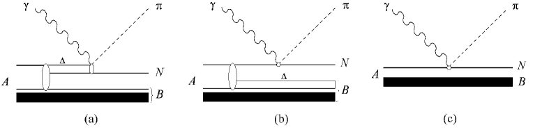
Figure 1: Diagrams illustrating the direct mechanisms of the pion production in the $A({\gamma,\,\pi N})B$ reaction.

The wave functions of the bound nucleon systems $\psi^{n_{N}}$ were calculated in the framework of the harmonic oscillator shell model, which reproduces the mean square charge radius of the nucleus.

A one-particle density matrix $\rho({X_{1};\tilde{X}_{1}})$ was analyzed in [10], taking into account the isobar configuration of the nuclear wave function. According to [10] direct mechanisms of the reaction $A({\gamma,\,\pi N})B$ are caused by the following components of the density matrix

$$\rho=\rho^{\Delta}+\rho^{N}+\rho^{C},$$ (4)

where

$$\rho^{\Delta}({X_{1};\tilde{X}_{1}})=\varphi_{\Delta}({m_{1}})\left[{\frac{{1}}{{A}}\sum\limits_{ij}{\int{dx_{2}}\,\psi_{[{\beta_{i}\beta_{j}}]}^{\Delta N}({x_{1},x_{2}})\psi_{[{\beta_{i}\beta_{j}}]}^{\Delta N\ast}({\tilde{x}_{1},x_{2}})}}\right]\varphi_{\Delta}^{\ast}({\tilde{m}_{1}}),$$ (5)

$$\rho^{N}({X_{1};\tilde{X}_{1}})=\varphi_{N}({m_{1}})\left[{\frac{{1}}{{A}}\sum\limits_{ij}{\int{dx_{2}}\,\psi_{[{\beta_{i}\beta_{j}}]}^{\Delta N}({x_{2},x_{1}})\psi_{[{\beta_{i}\beta_{j}}]}^{\Delta N\ast}({x_{2},\tilde{x}_{1}})}}\right]\varphi_{N}^{\ast}({\tilde{m}_{1}}),$$

$$\rho^{C}({X_{1};\tilde{X}_{1}})=\varphi_{N}({m_{1}})\left[\frac{{1}}{{A}}\left(N_{N}\sum\limits_{i=1}^{A}\psi_{\beta_{i}}(x_{1})\,\psi_{\beta_{i}}^{*}(\tilde{x}_{1})+\sum\limits_{ij,k\neq ij}N_{\Delta ij}\,\psi_{\beta_{k}}(x_{1})\,\psi_{\beta_{k}}^{*}(\tilde{x}_{1})\right)\right]\varphi_{N}^{\ast}({\tilde{m}_{1}}).$$

Here, $\psi_{\beta}({x})$ is the single-particle wave function of the bound nucleon in the nucleus in a state $\beta$ and $N_{\Delta}=\sum\nolimits_{ij}{N_{\Delta ij}}$, $N_{N}$ are the norms of the wave functions $\Psi_{\beta}^{\Delta}$ and $\Psi_{\beta}^{N}$.

In the context of equation (1), these components (4) of the density matrix correspond to the reaction mechanisms, which are illustrated by the diagrams in Figs. 1a, 1b and 1c.

The diagrams in Figs. 1a and 1b describe the mechanisms of the reactions, in which the production of the pion–nucleon pair occurs at the interaction of photon with the isobar and nucleon of the $\Delta$N system. The pion production as a result of the mechanism, corresponding to diagram 1c, occurs at the interaction of a photon with a nucleon of the nucleon core. In this case, the wave function of the residual nucleus B includes both the nucleon and isobar configurations.

Consider the second component of the model – the operator $t_{\gamma\pi}$. The operators of the pion production, acting in the spaces of the coordinates x and X, are related by the equation

$$<x^{\prime}|t_{\gamma B\to N\pi}|x>=\sum\limits_{{m}^{\prime},m}{\varphi_{N}^{\ast}({{m}^{\prime}})}<X^{\prime}|t_{\gamma\pi}|X>\varphi_{B}({m}).$$

Here, the internal state index B is N or $\Delta$. Using the S-matrix approach to the description of the $\gamma+\Delta\to N+\pi$ processes, transition operator $t_{\gamma\Delta\to N\pi}$ was found and it was presented as an expansion of four spin and three isospin independent structures with the expansion coefficients that depend on the coupling constants and magnetic moments. The single-particle transition operator $t_{\gamma\Delta\to N\pi}$ is determined by the $\gamma+\Delta\to N+\pi$ process amplitude [10] that can be graphically represented as a sum of the diagrams shown in Fig. 2.

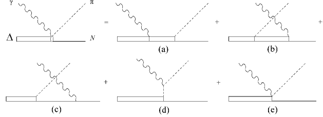
Figure 2: Diagrams for describing the $\gamma\Delta\to N\pi$ process.

At the interaction of a photon with isobars $\Delta^{++},\ \Delta^{+}$ and $\Delta^{-}$ the amplitude corresponding to the diagram in Fig. 2a dominates in the kinematic region of the $\Delta$(1232). At the interaction of photon with neutral isobar $\Delta^{0}$ this diagram does not contributes to the transition amplitude, but the amplitude corresponding to the contact diagram in Fig. 2e dominates. As the single-particle transition operator $t_{\gamma N\to N^{\prime}\pi}$, we will use the non-relativistic Blomqvist–Laget photoproduction operator [14].

In accordance with (4),

$$\sum\limits_{f_{B}}{\left|{T_{d}^{\Delta N}}\right|^{2}}=\sum\limits_{f_{B}}{\left|{T_{d}^{\Delta}}\right|^{2}+\left|{T_{d}^{N}}\right|^{2}}+\left|{T_{d}^{C}}\right|^{2}.$$ (6)

Considering the first term of this expression, we then in (5) express the wave function $\psi_{[{\beta_{i}\beta_{j}}]}^{\Delta N}({x_{1},x_{2}})$ of the $\Delta$N system through its Fourier transform $\xi_{[{\beta_{i}\beta_{j}}]}^{\Delta N}({y_{1},y_{2}})$, where $y\equiv{\bf p},s,t$,

$$\psi_{[{\beta_{i}\beta_{j}}]}^{\Delta N}({x_{1},x_{2}})=\frac{{1}}{{({2\pi})^{3}}}\int{d({{\bf p}_{1},{\bf p}_{2}})}\exp\left({i({{\bf p}_{1}{\bf r}_{1}+{\bf p}_{2}{\bf r}_{2}})}\right)\,\xi_{[{\beta_{i}\beta_{j}}]}^{\Delta N}({y_{1},y_{2}})$$

and represent $\xi_{[{\beta_{i}\beta_{j}}]}^{\Delta N}({y_{1},y_{2}})$ in the form of an expansion in states of the $\Delta$N system with total angular momentum J, isospin T, the orbital angular momentum l, total spin s and its projections M_J, M_T, m_l and m_s as

$$\xi_{[{\beta_{i}\beta_{j}}]}^{\Delta N}({y_{1}y_{2}})=\sum\limits_{\beta_{S}}{\Psi_{[{\beta_{i}\beta_{j}}]\beta_{S}}^{\Delta N}({\bf P},{\bf p})}\,\Omega_{\beta_{S}}({s_{1},s_{2},t_{1},t_{2}}).$$ (7)

Here, $\beta_{S}$ $\equiv$ $({\beta_{ex}\equiv J,M_{J},T,M_{T}}),({\beta_{in}\equiv l,s})$, ${\bf P}={\bf p}_{1}+{\bf p}_{2}$ is the momentum of the $\Delta$N system, ${\bf p}=({\bf p}_{1}M_{N}-{\bf p}_{2}M_{\Delta})/(M_{\Delta}+M_{N})$ is the relative momentum, $M_{\Delta}$ and $M_{N}$ are isobar and nucleon masses, respectively and $\Omega_{\beta_{S}}$ is the spin–isospin wave function of the $\Delta$N system.

As a result, after integration over internal, spin and isospin coordinates, the squared modulus of the amplitude $T_{d}^{\Delta}$ summed over the states f_B of the residual nucleus B and the spin states f_n of the nucleon, can be written as

$$\sum\limits_{f_{B},f_{n}}{\left|{T_{d}^{\Delta}}\right|^{2}}=\,({2\pi})^{3}\mbox{Sp}({t_{\gamma\Delta\to N\pi}\,\bm{\rho}_{p}^{\Delta}({{\bf{p}}_{\Delta}})\,t_{\gamma\Delta\to N\pi}^{\dagger}})\,\mbox{Sp}({R_{m\tau_{\Delta}}^{\Delta}({{\bf{p}}_{\Delta}})}),$$ (8)

where

$$\bm{\rho}_{p}^{\Delta}({\bf{p}})=\frac{{R_{m\tau_{\Delta}}^{\Delta}({\bf{p}})}}{{\mbox{Sp}({R_{m\tau_{\Delta}}^{\Delta}({\bf{p}})})}}$$

is the polarization density matrix,

$$R_{m\tau_{\Delta}}^{\Delta}({{\bf{p}}_{\Delta}})=\sum\limits_{\beta_{ex}\beta_{in}\tilde{\beta}_{in}}{\int{d{\bf{P}}}}\,U_{\beta_{ex}\beta_{in}\tilde{\beta}_{in}}({\hat{\bf{p}}})\,\rho_{m\tau_{\Delta},\beta_{ex}\beta_{in}\tilde{\beta}_{in}}^{\Delta}({{\bf{P}},p}),$$ (9)

$$U_{\beta_{ex}\beta_{in}\tilde{\beta}_{in}}^{m\sigma_{\Delta}m\tilde{\sigma}_{\Delta}}({\hat{\bf{p}}})=\sum\limits_{m\sigma_{N}}{S_{\beta_{ex}\beta_{in}\tilde{\beta}_{in}}^{m\sigma_{\Delta}m\tilde{\sigma}_{\Delta}m\sigma_{N}m\sigma_{N}}({\hat{\bf{p}}})},$$

$$\rho_{m\tau_{\Delta},\beta_{ex}\beta_{in}\tilde{\beta}_{in}}^{\Delta}({{\bf{P}},{{p}}})=\sum\limits_{m\tau_{N}}{\rho_{m\tau_{\Delta}m\tau_{N},\beta_{ex}\beta_{in}\tilde{\beta}_{in}}({{\bf{P}},{{p}}})},$$

$$S_{\beta_{ex}\beta_{in}\tilde{\beta}_{in}}^{m\sigma_{\Delta}m\tilde{\sigma}_{\Delta}m\sigma_{N}m\tilde{\sigma}_{N}}({\hat{\bf{p}}})=\sum\limits_{m_{l},\tilde{m}_{l}}{Y_{l,m_{l}}({\hat{\bf{p}}})Y_{\tilde{l},\tilde{m}_{l}}^{\ast}({\hat{\bf{p}}})}\sum\limits_{m_{s},\tilde{m}_{s}}{C_{l,m_{l};s,m_{s}}^{J,M_{J}}C_{{{3}\mathord{\left/{\vphantom{{3}{2}}}\right.\kern-1.2pt}{2}},m\sigma_{\Delta};{{1}\mathord{\left/{\vphantom{{1}{2}}}\right.\kern-1.2pt}{2}},m\sigma_{N}}^{s,m_{s}}}C_{\tilde{l},\tilde{m}_{l};\tilde{s},\tilde{m}_{s}}^{J,M_{J}}C_{{{3}\mathord{\left/{\vphantom{{3}{2}}}\right.\kern-1.2pt}{2}},m\tilde{\sigma}_{\Delta};{{1}\mathord{\left/{\vphantom{{1}{2}}}\right.\kern-1.2pt}{2}},m\tilde{\sigma}_{N}}^{\tilde{s},\tilde{m}_{s}},$$

$$\rho_{m\tau_{\Delta}m\tau_{N},\beta_{ex}\beta_{in}\tilde{\beta}_{in}}({{{\bf{P}},{{p}}}})=\sum\limits_{ij}{\psi_{[{\beta_{i}\beta_{j}}]\beta_{ex}\beta_{in}}^{\Delta N}({{{\bf{P}},{{p}}}})\,\psi_{[{\beta_{i}\beta_{j}}]\beta_{ex}\tilde{\beta}_{in}}^{\Delta N\ast}({{{\bf{P}},{{p}}}})\left|{C_{{{3}\mathord{\left/{\vphantom{{3}{2}}}\right.\kern-1.2pt}{2}},m\tau_{\Delta};{{1}\mathord{\left/{\vphantom{{1}{2}}}\right.\kern-1.2pt}{2}},m\tau_{N}}^{T,M_{T}}}\right|^{2}}.$$

Here, $m\tau_{\Delta}=m\tau_{\pi}+m\tau_{n}$ is the third projection of the isobar isospin, ${\bf{p}}_{\Delta}={\bf{p}}_{\pi}+{\bf{p}}_{n}-{\bf{p}}_{\gamma}$ is the isobar momentum satisfying equality in (9)

$${\bf{p}}={\bf{p}}_{\Delta}-\frac{{M_{\Delta}}}{{M_{\Delta}+M_{N}}}{\bf{P}}.$$

In equation (7), the wave function $\Psi_{[{\beta_{i}\beta_{j}}]\beta_{S}}^{\Delta N}({{\bf{P}},{\bf{p}}})$ is associated with the function $\psi_{[{\beta_{i}\beta_{j}}]\beta_{ex}\beta_{in}}^{\Delta N}({{{\bf{P}},{p}}})$ by the relation

$$\Psi_{[{\beta_{i}\beta_{j}}]\beta_{S}}^{\Delta N}({{{\bf{P}},{\bf{p}}}})=\psi_{[{\beta_{i}\beta_{j}}]\beta_{ex}\beta_{in}}^{\Delta N}({{{\bf{P}},{p}}})Y_{l,m_{l}}({\hat{\bf{p}}}).$$

The trace of the matrix $R_{m\tau_{\Delta}}^{\Delta}$ is

$$\mbox{Sp}({R_{m\tau_{\Delta}}^{\Delta}({{\bf{p}}_{\Delta}})})=\frac{{1}}{{4\pi}}\sum\limits_{\beta_{S}}{\int{d{\bf{P}}}}\,\rho_{m\tau_{\Delta},\beta_{ex}\beta_{in}\beta_{in}}^{\Delta}({{\bf{P}},{{p}}})=\rho_{m\tau_{\Delta}}^{\Delta}({{\bf{p}}_{\Delta}}).$$

Here, $\rho_{m\tau_{\Delta}}^{\Delta}({{\bf{p}}_{\Delta}})$ is the momentum distribution of the isobar in the charge state $m\tau_{\Delta}+0.5$.

Undertaking a similar transformation for the second term of (6), we obtain

$$\sum\limits_{f_{B},f_{n}}{\left|{T_{d}^{N}}\right|^{2}}=\,({2\pi})^{3}\mbox{Sp}({t_{\gamma N\to N^{\prime}\pi}\,\bm{\rho}_{p}^{N}({{\bf{p}}_{N}})t_{\gamma N\to N^{\prime}\pi}^{+}})\times\,\mbox{Sp}({R_{m\tau_{N}}^{N}({{\bf{p}}_{N}})}),$$ (10)

where $m\tau_{N}=m\tau_{\pi}+m\tau_{n}$ is the third isospin projection of the nucleon of the $\Delta$N system,

$$\bm{\rho}_{p}^{N}({\bf{p}})=\frac{{R_{m\tau_{N}}^{N}({\bf{p}})}}{{\mbox{Sp}({R_{m\tau_{N}}^{N}({\bf{p}})})}},$$

$$R_{m\tau_{N}}^{N}({{\bf{p}}_{N}})=\sum\limits_{\beta_{ex}\beta_{in}\tilde{\beta}_{in}}{\int{d{\bf{P}}}}\,V_{\beta_{ex}\beta_{in}\tilde{\beta}_{in}}({\hat{\bf{p}}})\rho_{m\tau_{N},\beta_{ex}\beta_{in}\tilde{\beta}_{in}}^{N}({{\bf{P}},{{p}}}),$$ (11)

$$V_{\beta_{ex}\beta_{in}\tilde{\beta}_{in}}^{m\sigma_{N}m\tilde{\sigma}_{N}}({\hat{\bf{p}}})=\sum\limits_{m\sigma_{\Delta}}{S_{\beta_{ex}\beta_{in}\tilde{\beta}_{in}}^{m\sigma_{\Delta}m\sigma_{\Delta}m\sigma_{N}m\tilde{\sigma}_{N}}({\hat{\bf{p}}})},$$

$$\rho_{m\tau_{N},\beta_{ex}\beta_{in}\tilde{\beta}_{in}}^{N}({{{\bf{P}},{{p}}}})=\sum\limits_{m\tau_{\Delta}}{\rho_{m\tau_{\Delta}m\tau_{N},\beta_{ex}\beta_{in}\tilde{\beta}_{in}}({{{\bf{P}},{{p}}}})}.$$

The relative momentum p in (11) is related to the nucleon momentum ${\bf{p}}_{N}={\bf{p}}_{\pi}+{\bf{p}}_{n}-{\bf{p}}_{\gamma}$ of the $\Delta$N system through the equation

$${\bf{p}}=-\,{\bf{p}}_{N}+\frac{{M_{N}}}{{M_{\Delta}+M_{N}}}\,{\bf{P}}.$$

Now consider the last term of equation (6). For the p-shell nuclei having a large set of nucleon states, the third component of the density matrix (4) can be written as

$$\rho^{C}({X_{1};\tilde{X}_{1}})=\varphi_{N}({m_{1}})\left[\frac{{N_{C}^{\Delta N}}}{{A}}\sum\limits_{i=1}^{A}\psi_{\beta_{i}}(x_{1})\,\psi_{\beta_{i}}^{*}(\tilde{x}_{1})\right]\varphi_{N}^{\ast}({\tilde{m}_{1}}),$$ (12)

where

$$N_{C}^{\Delta N}=N_{N}+N_{\Delta}\,\frac{A-2}{A}.$$

Using (12), we obtain

$$\sum\limits_{f_{B},f_{n}}{\left|{T_{d}^{C}}\right|^{2}}=\,({2\pi})^{3}\mbox{Sp}({t_{\gamma N\to N^{\prime}\pi}\,{}t_{\gamma N\to N^{\prime}\pi}^{\dagger}})\frac{{1}}{{2\,\sigma_{N}+1}}\,\rho_{m\tau_{N}}^{C}({{\bf{p}}_{N}}).$$ (13)

Here, $\sigma_{N}$ is the nucleon spin,

$$\rho_{m\tau_{N}}^{C}({{\bf{p}}_{N}})=N_{C}^{\Delta N}\sum\limits_{i=1}^{A}{\,\left|{\psi_{\beta_{i}}({{\bf{p}}_{N}})}\right|^{2}{}}\,\delta_{m\tau_{N},m\tau_{i}}$$ (14)

is the momentum distribution of the nucleons with the third isospin projection $m\tau_{N}$, constituting the nucleon core of the nucleus, and $\psi_{\beta}({\bf{p}})$ is the Fourier transform of the spatial part of the wave function $\psi_{\beta}({x})$.

Equation (13), for the squared modulus of amplitude $T_{d}^{C}$, differs from similar expression obtained in the quasifree approximation, taking into account the nucleon configurations of the nuclear wave function only, by the presence of the factor $N_{C}^{\Delta N}$. For the ¹⁶O nucleus factor $N_{C}^{\Delta N}$ is equal to 0.97.

Now we consider the quasifree pion photoproduction model, taking into account the isobar configurations in the ground state of the nuclei. In this approach, the independent particle model is used as a model of a nucleus, and the isobars and nucleons in the nucleus are considered as independent constituents. In this model the wave function of the isobar configurations of a nucleus with closed shells can be represented as

$$\Psi_{\beta}^{\Delta}({X_{1},...,X_{A}})=A_{\Delta}\sum\limits_{i}{\Psi_{\beta_{i}}^{\Delta}({X_{1}})\Psi_{({\beta_{i}})^{-1}}^{N}({X_{2},X_{3},...,X_{A}})}$$ (15)

where $\Psi_{\beta}^{\Delta}({X})=\varphi_{\Delta}({m})\,\psi_{\beta}^{\Delta}({x})$ is the wave function of the virtual isobar in the nucleus in the $\beta$ state and $\Psi_{({\beta})^{-1}}^{N}$ is the wave function of the nucleon core including $A-1$ nucleons, whose state can be described in terms of the oscillator shell model.

If we use equation (15) for the wave function of the isobar configurations, the squared modulus of the amplitude $T_{qf}$ in the quasifree approximation, summed over the residual nucleus states f_B and the nucleon spin states f_n, can be written, as

$$\sum\limits_{f_{B},f_{n}}{\left|{T_{qf}}\right|^{2}}=\sum\limits_{f_{B},f_{n}}{\left|{T_{qf}^{\Delta}}\right|^{2}}+\left|{T_{qf}^{C}}\right|^{2},$$ (16)

where

$$\sum\limits_{f_{B},f_{n}}{\left|{T_{qf}^{\Delta}}\right|^{2}}=\,({2\pi})^{3}\mbox{Sp}({t_{\gamma\Delta\to N\pi}\,t_{\gamma\Delta\to N\pi}^{\dagger}})\frac{1}{2\,\sigma_{\Delta}+1}\,\rho_{m\tau_{\Delta}}^{\Delta}({{\bf{p}}_{\Delta}}),$$ (17)

$$\rho_{m\tau_{\Delta}}^{\Delta}({\bf{p}})=\sum\limits_{i}{\left|{\psi_{\beta_{i}}^{\Delta}({\bf{p}})}\right|^{2}{}}\delta_{m\tau_{\Delta},m\tau_{i}}.$$

Here, $\sigma_{\Delta}$ is the isobar spin and $\psi_{\beta}^{\Delta}({\bf{p}})$ is the Fourier transform of the spatial part of the isobar wave function $\psi_{\beta}^{\Delta}({x})$.

The formula for the squared modulus of the amplitude $T_{qf}^{C}$ coincides with (13). The difference lies in the value of the coefficient that determines the momentum distribution of the nucleons in the nucleus (14). The factor $N_{C}^{\Delta N}$ in (14) should be replaced by

$$N_{C}^{qf}=N_{N}+N_{\Delta}\,\frac{A-1}{A}.$$

The coefficients $N_{C}^{qf}$ and $N_{C}^{\Delta N}$ differ by a value $N_{\Delta}/A$, which essentially does not exceed $\sim$0.02 for the p-shell nuclei [6, 11].

3 Results and discussion

Depending on the charge state of the $\pi$N pair, produced in the $A({\gamma,\,\pi N})B$ reaction, a main contribution to the cross section is given by different elements in equations (6) and (16). In particular, the non-zero contribution to the production of the $\pi^{+}p$ or the $\pi^{-}n$ pairs give only the first terms corresponding to the interaction of a photon with the $\Delta^{++}$ or $\Delta^{-}$ isobars. In the case of the $\pi^{+}n,\,\pi^{0}p,\,\pi^{0}n$ and $\pi^{-}p$ pair production with an electric charge equal to 0 or +1, all terms in (6) and (16) contribute to the cross section. For example, at production of the $\pi^{-}p$ pair, the first terms in (6) and (16) correspond to the production of the pion in the process $\gamma\Delta^{0}\to\pi^{-}p$; the second term in (6), which is absent in the quasifree pion production model, corresponds to the production of the pion in the process $\gamma n\to\pi^{-}p$ at the interaction of the photon with neutron of the $\Delta^{0}n$, $\Delta^{+}n$ and $\Delta^{++}n$ correlated systems. The last terms in (6) and (16) describe the contribution to the cross section of the $\pi^{-}$ photoproduction on the neutrons of the nucleon core.

Figure 3: Differential cross section of the reaction ¹⁶O$({\gamma,\,\pi^{+}p}){}^{15}$C as a function of the momentum p_B of the residual nucleus ¹⁵C at $E_{\gamma}=450\,$MeV, $\theta_{\pi}^{\ast}=\varphi_{\pi}=\theta_{B}=90^{\circ}$. The solid curve is the $\Delta$N correlation model; the dashed curve is the quasifree pion photoproduction model. The calculations were undertaken in plane-wave approximation.

Figure 4: Differential cross section of the reaction ¹⁶O$({\gamma,\,\pi^{+}p})^{15}$C as a function of the polar angle $\theta_{B}$ of the emission of the residual nucleus ¹⁵C at $E_{\gamma}=450\,$MeV, $\theta_{\pi}^{\ast}=\varphi_{\pi}=90^{\circ}$, $p_{B}=370\,\mbox{MeV}/c$. Designation of the curves is the same as in Fig. 3.

Consider a prediction of the models for the two reactions ¹⁶O$({\gamma,\,\pi^{+}p}){}^{15}$C and ¹⁶O$({\gamma,\,\pi^{-}p}){}^{15}$O.

The single mechanism of the direct production of the $\pi^{+}$p pair in the $({\gamma,\,\pi^{+}p})$ reaction is represented by the diagram in Fig. 1a. Comparing formulas (8) and (17) for the squared modulus of the amplitude $T^{\Delta}$, we note that the expression Sp$({t_{\gamma\Delta\to N\pi}\,\bm{\rho}_{p}^{\Delta}\,t_{\gamma\Delta\to N\pi}^{\dagger}})$ in (8) is the squared modulus of the matrix element of the transition $\gamma\Delta\to N\pi$, summed over the spin states of the isobar and nucleon, which describes the interaction of a photon with the polarized isobar. The polarization state of the isobar is determined by the polarization density matrix $\bm{\rho}_{p}^{\Delta}$.

The polarization density matrix $\bm{\rho}_{m\tau_{\Delta}}^{\Delta}$can be expanded in the polarization operators [15] and can be presented in its simplest form as

$$\bm{\rho}_{p}^{\Delta}=\frac{{1}}{{2\sigma_{\Delta}+1}}({I+\Sigma}),$$

where $I$ is the unity matrix, having the dimension $({2\sigma_{\Delta}+1})\times({2\sigma_{\Delta}+1})$. If the isobar is not polarized, the second term $\Sigma=0$. Thus, ignoring the effective polarization of the isobar in the initial state of the process $\gamma\Delta\to N\pi$, we obtain for the first term of (6) a natural transition from the model taking into account the $\Delta$N correlations, to an approach based on the independent particle model. The origin of the effective polarization of the isobar in the $({\gamma,\,\pi N})$ process is related to the fact, that in the wave function expansion (7), the magnitude of the $\Delta$N state contribution depends on the value $m\sigma_{\Delta}$. A degree of influence of the effective isobar polarization on the cross section of the ¹⁶O$({\gamma,\,\pi^{+}p}){}^{15}$C reaction can be estimated on the basis of the data presented in Figs. 3, 4 and 5.

As we know, within the framework of the quasifree pion photoproduction, polarization effects arise from the final state interaction [16, 17]. To assess the effect of the polarization caused only by the $\Delta$N correlations, calculations were performed in the plane-wave approximation.

Fig. 3 shows the dependence of the differential cross section of the ¹⁶O$({\gamma,\pi^{+}p}){}^{15}$C reaction plotted against the momentum of the residual nucleus ¹⁵C. The calculations were undertaken in the following kinematic region: photon energy of 450 MeV, pion momentum in the c.m. of the pion-nucleon pair perpendicular to the photon momentum, polar angle $\theta_{B}$ of the residual nucleus emission and azimuth angle $\varphi_{\pi}$ of pion emission in the laboratory frame equal to 90^∘; it was assumed that the geometry was coplanar and that the positive and negative values of the momentum on the x-axis corresponded to the azimuth angles $\varphi_{B}$ of the emission of the residual nucleus ¹⁵C equal to $+90^{\circ}$ and $-90^{\circ}$. The solid curve in Fig. 3 shows the reaction cross section calculated using the $\Delta$N correlation model, and the dashed curve is the cross section calculated in the framework of the quasifree pion photoproduction model. According to [3, 18], it was assumed that the $\Delta$N system produced upon the $NN\rightarrow\Delta N$ transition was in a state, whose quantum numbers were J = 0, T = 1, and l = s = 2. Significant asymmetry of the cross section with respect to zero on the x-axis is mainly due to an asymmetric contribution of the diagram in Fig. 2a to the transition amplitude $\gamma\Delta^{++}\to p\pi^{+}$.

Figure 5: Differential cross section of the reaction ¹⁶O$({\gamma,\,\pi^{+}p}){}^{15}$C as a function of the azimuth angles $\varphi_{B}$ of the residual ¹⁵C nucleus emission at $E_{\gamma}=\mbox{MeV},\ \theta_{\pi}^{\ast}=\varphi_{\pi}=90^{\circ},\ p_{B}=370\,\mbox{MeV}/c$. Designation of the curves is the same as in Fig. 3.

Figs. 4 and 5 show the dependences of the differential cross section of the reaction ¹⁶O$({\gamma,\,\pi^{+}p}){}^{15}$C plotted against the polar $\theta_{B}$ and azimuth $\varphi_{B}$ angles of the residual nucleus emission. The kinematic situation is different from the previous case. In Fig. 4 the momentum of the residual nucleus is fixed and it is equal to 370 MeV/c, and in Fig. 5, additionally, the polar angle $\theta_{B}$ is fixed and it equals 90^∘. Positive and negative values of the variable on the abscissa in Fig. 4 correspond to the azimuth angles $\varphi_{B}$ of emission of the residual nucleus ¹⁵C as well as in Fig. 3. In Fig. 5 the momenta of particles participating in the reaction are coplanar when the azimuth angles $\varphi_{B}$ are 90^∘ and 270^∘.

As can be seen, outside the scope of the coplanarity of the particle momenta, a difference in the differential cross sections of the ¹⁶O$({\gamma,\,\pi^{+}p}){}^{15}$C reaction calculated in the two models, reaches $\sim$ 80%.

We now proceed to the analysis of the reaction ¹⁶O$({\gamma,\,\pi^{-}p}){}^{15}$O.

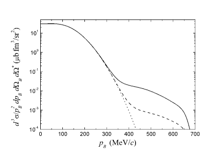
Figure 6: Differential cross section of the reaction ¹⁶O$({\gamma,\,\pi^{-}p})^{15}$O as a function of the momentum $p_{B}$ of the residual nucleus ¹⁵O at $E_{\gamma}=450\,\mbox{MeV},\ \theta_{\pi}^{\ast}=\varphi_{\pi}=\theta_{B}=90^{\circ}$, $\varphi_{B}=-90^{\circ}$. The solid curve is the $\Delta$N correlation model, the dashed curve is the quasifree pion photoproduction model and the dotted line is the contribution to the cross section of the $T_{d}^{C}$ and $T_{qf}^{C}$ amplitudes corresponding to the interaction of the photons with the neutrons of the nucleon core. The calculation was undertaken in plane-wave approximation.

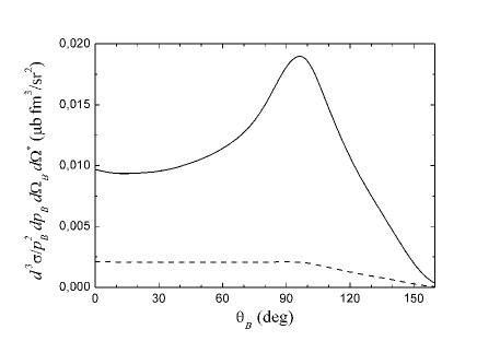
Figure 7: Differential cross section of the reaction ¹⁶O$({\gamma,\,\pi^{-}p}){}^{15}$O as a function of the polar angle $\theta_{B}$ of the residual nucleus ¹⁵O at $E_{\gamma}=450\,\mbox{MeV},\ p_{B}=400\,\mbox{MeV}/c,\ \theta_{\pi}^{\ast}=\varphi_{\pi}=90^{\circ},\ \varphi_{B}=-90^{\circ}.$ Designation of the curves is the same as in Fig. 6.

In Fig. 6 we show the dependence of the differential cross section of the ¹⁶O$({\gamma,\,\pi^{-}p}){}^{15}$O reaction plotted against the momentum $p_{B}$ of the residual nucleus ¹⁵O at $E_{\gamma}=450\,\mbox{MeV},\,\theta_{\pi}^{\ast}=\varphi_{\pi}=\theta_{B}=90^{\circ}$, $\varphi_{B}=-90^{\circ}$. The significant difference in process $({\gamma,\,\pi^{-}p})$ from process $({\gamma,\,\pi^{+}p})$ is that the $\pi^{-}p$ pair production is possible at the interaction of a photon with the nucleons. Therefore, the contribution to the reaction cross section is possible from all terms in (6) and (16).

Figure 8: Differential cross section of the reaction ¹⁶O$({\gamma,\pi^{-}p})$ as a function of the kinetic energy of the proton T_p. Data are taken from Ref. [13]. The dotted and dashed-dotted curves are the contributions to the cross section of the nucleon core and the isobar configurations respectively, the dashed-dotted-dotted curve is the sum of the cross section of the ¹⁶O$({\gamma,\,\pi^{-}p})n{}^{14}$O and ¹⁶O$({\gamma,\,\pi^{-}p})p{}^{14}$N reaction, the solid curve is the sum of the cross section of the $\pi^{-}$ photoproduction with the one- and two-nucleons emissions. The calculation was undertaken in distorted wave approximation.

The dotted curve in Fig. 6 shows the contribution to the cross section of the pion photoproduction on the neutrons, corresponding amplitudes $T_{d}^{C}$ and $T_{qf}^{C}$, which, under minor differences in magnitude, dominate at small momenta of the residual nucleus. The solid and dashed curves show the differential cross section calculated with the help of the $\Delta$N correlation model and the quasifree pion photoproduction model, respectively, taking into account the isobar configurations in the ground state of a nucleus. As can be seen, at momenta of the residual nucleus above $\sim$400 MeV/c, the $\pi^{-}p$ pair production is almost entirely due to the isobar configurations and the differential cross sections, obtained in the framework of the two models under consideration, differ in this kinematic region by almost one order of magnitude.

Fig. 7. shows the differential cross section of the reaction ¹⁶O$({\gamma,\,\pi^{-}p}){}^{15}$O plotted against polar angle $\theta_{B}$ of the residual nucleus ¹⁵O at $E_{\gamma}=450\,\mbox{MeV},$ $p_{B}=400\,\mbox{MeV}/c,\ \theta_{\pi}^{\ast}=\varphi_{\pi}=90^{\circ},\ \varphi_{B}=-90^{\circ}.$ As can be seen, the two models predict the differential cross section, significantly differing both in an absolute value and in the shape of the angular dependence.

Currently, there are no experimental data for the reaction $A({\gamma,\,\pi N})B,$ that would produce a conclusion about the validity of the considered reaction models. There are exclusive experimental cross sections measured at a particular state of the residual nucleus [19, 20, 21]. However, these data were obtained in the region of small momenta of the residual nucleus, where the contribution of the isobar configurations is disparagingly small. There are experimental data measured in the region of high-momentum transferred to the residual nucleus, but without restriction on the missing energy [13, 22, 23]. Therefore, these data include the final state in which the residual nucleus is disintegrated. Such experimental data of the $({\gamma,\,\pi^{+}p})$ reaction measured at the Tomsk synchrotron have recently been satisfactorily interpreted using the model of reactions $({\gamma,\,\pi N})$ and $({\gamma,\,\pi NN})$ taking into account the $\Delta$N correlations in the ground state of the nuclei [11]. Below we use this approach to analyze the ¹⁶O$({\gamma,\,\pi^{-}p})$ reaction data measured at the BNL LEGS [13].

Fig. 8 shows the differential cross section of the reaction ¹⁶O$({\gamma,\,\pi^{-}p})$ plotted against kinetic energy of the proton T_p at $E_{\gamma}\simeq 300\,$MeV, (a) $\theta_{\pi}=44^{\circ},\ \theta_{p}=55^{\circ};$ (b) $\theta_{\pi}=36^{\circ},\ \theta_{p}=75^{\circ};$ (c) $\theta_{\pi}=132^{\circ},\ \theta_{p}=75^{\circ}.$ We chose the cross section data from the large amount of data obtained in the experiment in [13], in which the average momentum $p_{B}$ transferred to the residual nuclear system is approximately equal to (a) 200 MeV/c, (b) 300 MeV/c, and (c) 400 MeV/c. In this range of the momentum transfers, the differential cross section of the quasifree pion photoproduction on the neutrons bound in a nucleus varies by more than an order of magnitude.

The theoretical cross section shown in Fig. 8 was calculated using the $\Delta$N correlation model, which includes the direct and exchange reaction mechanisms [10, 12]. The final state interaction was taken into account in the optical model. The dotted curve shows the cross section of the $\pi^{-}$ photoproduction in the reaction ¹⁶O$({\gamma,\,\pi^{-}p}){}^{15}$O on neutrons of the nucleon core (contribution of the amplitude $T^{C}$). The dashed-dotted curve shows the contribution to the cross section of the ¹⁶O$({\gamma,\,\pi^{-}p})^{15}$O reaction of the isobar configurations in the ground state of the nucleus ¹⁶O. The dashed-dotted-dotted curve is the sum of the cross sections of the ¹⁶O$({\gamma,\,\pi^{-}p})n{}^{14}$O and ¹⁶O$({\gamma,\,\pi^{-}p})p{}^{15}$N reactions. In the kinematic region considered above, the contribution of the isobar configurations in the reaction ¹⁶O$({\gamma,\,\pi^{-}p})^{15}$O in the framework of the quasifree pion photoproduction does not exceed 10^-1 nb/MeV sr². The solid curve shows the sum of the the $\pi^{-}$ photoproduction cross sections with the emission of one and two nucleons. As can be seen, considering the isobar configurations, we satisfactorily reproduced the form of the energy dependence of the reaction cross section. However, disagreement of the absolute values of the experimental data and theoretical cross sections increases with the growth in the momentum of the residual nuclear system. At average momentum $p_{B}\approx 400$ MeV/c, the experimental differential cross section exceeds the calculated cross section more than three-fold.

4 Conclusions

We have considered two models of the $A({\gamma,\,\pi N})B$ reaction that take into account the isobar configurations in the ground state of an atomic nucleus: the $\Delta$N correlation model and the quasifree pion photoproduction model. The main distinction between the two models is the description of the state of an atomic nucleus, which comprises the isobars. The general feature for these models is the approach, in accordance with which isobars and nucleons are equal components of an atomic nucleus. Distinction between the models consists of the following: in the $\Delta$N correlation model, the dynamic relationship between the nucleon and the isobar of the $\Delta$N system, formed in the virtual transition $NN\to\Delta N$, is taken into account. In the quasifree pion production model, the independent particle model is used – nucleons and isobars in a nucleus are considered independent. In the $\Delta$N correlation model, the photon interacts with baryons in three states: isobar, nucleon of the $\Delta$N system and nucleons of the nucleon core. In the quasifree pion production model, there are only two such baryon states. This leads to the main difference between the two models of the $A({\gamma,\,\pi N})B$ reaction – the additional amplitude $T_{d}^{N}$ (10) in the $\Delta$N correlation model, which provides a significant contribution to the cross section of the production of the pion–nucleon pair with charge 0 and +1 at high momenta of the residual nucleus. Another difference between the predictions of the two models is the presence of the polarization density matrix $\bm{\rho}_{p}^{\Delta}$, in the expression for the squared modulus of the amplitude $T^{\Delta}$ (8), which describes the interaction of a photon with the isobar within the $\Delta$N correlation model. Effective polarization of the virtual isobar in the nucleus has a significant impact on the value of the reaction cross section.

As is known, the quasifree pion photoproduction model satisfactorily describes the reaction $A({\gamma,\,\pi N})B$ at sufficiently high momenta, transferred to the nucleon in the process $\gamma N\to N^{\prime}\pi$, and the small momenta of the residual nucleus, where the contribution of the nucleon configurations dominates [24, 25, 26]. The independent particle model reproduces well the manifestations in the reaction of the shell structure of the nucleus. However, a description of the state of the nucleus, which includes the isobar configurations, within the framework of the independent particle model, seems questionable. Because of the short lifetime of the isobars, it is unlikely that, after its appearance, the remaining $A-1$ nucleons form a collective state with the equilibrium momentum distribution, independent of the state of the isobar. The $\Delta$N correlation model eliminates this controversial hypothesis by analyzing the state of the $\Delta$N system, formed in the transition $NN\to\Delta N$. In this model, the states of the nucleon and isobar of the $\Delta$N system are interdependent. Thus, the $\Delta$N correlation model is physically more justified.

Due to the current lack of experimental data for the exclusive $A({\gamma,\,\pi N})B$ reactions at high momenta of the residual nucleus, we cannot form an unambiguous conclusion about the validity of the considered reaction models. However, a satisfactory description of the $({\gamma,\pi^{+}p})$ reaction data at the high momenta of the residual nuclear system, with the help of the $\Delta$N correlation approach, is evidence in favor of the $\Delta$N correlation model [11]. As has been shown, the $\Delta$N correlation model of the $({\gamma,\,\pi N})$ and $({\gamma,\,\pi NN})$ reactions also improves the description of the ¹⁶O$({\gamma,\,\pi^{-}p})$ reaction data measured at BNL [13]. The observed excess of the experimental data of the ¹⁶O$({\gamma,\pi^{-}p})$ reaction over the theoretical cross sections is connected, possibly, with a contribution of reaction mechanisms to the emission of two nucleons, which are described by a model with two-body transition operators – meson exchange currents.

References

• [1] A. M. Green, Rep. Progr. Phys. 39, 1109 (1976).
• [2] H. J. Weber and H. ArenhΓΆvel, Phys. Rep. 36, 277 (1978).
• [3] G. Horlacher and H. ArenhΓΆvel, Nucl. Phys. A 300, 348 (1978).
• [4] T. Frick, S. Kaiser, H.MΓΌther, et al., Phys. Rev. C 65, 034316 (2002).
• [5] C. I. Morris, J. D. Zumbro, J. A. McGill, et al., Phys. Lett. B 419, 25 (1998).
• [6] E. A. Pasyuk, R. L. Boudrie, P. A.Gram, et al., Phys. Lett. B 523, 1 (2001).
• [7] A. I. Amelin, M. N. Behr, B. A. Chernyshev, et al., Phys. Lett. B 337, 261 (1994).
• [8] A. Fix, I. Glavanakov, and Yu. Krechetov, Nucl. Phys. A 646, 417 (1999).
• [9] V. M. Bystritsky, A. I. Fix, I. V. Glavanakov, et al., Nucl. Phys. A 705, 55 (2002).
• [10] I. V. Glavanakov and A. N. Tabachenko, Nucl. Phys. A 889, 51 (2012).
• [11] I.V. Glavanakov, P. Grabmayer, Yu.F. Krechetov, and A.N. Tabachenko, JETP Lett. 97, 173 (2013).
• [12] I. V. Glavanakov and A. N. Tabachenko, Nucl. Phys. A 915, 179 (2013).
• [13] K. Hicks, V. Gladyshev, H. Baghaei, et al., Phys. Rev. C 61, 054609 (2000).
• [14] I. Blomqvist and J. M. Laget, Nucl. Phys. A 280, 405 (1977).
• [15] D. A. Varshalovich, A. N. Moskalev, and V. K. Khersonskii Quantum Theory of Angular Momentum (World Sci., Singapore, 1988).
• [16] J. M. Laget, Nucl. Phys. A 194, 81 (1972).
• [17] I. V. Glavanakov, Sov. J. Nucl. Phys. 55, 1508 (1992).
• [18] A. N. Tabachenko, Russ. Phys. J. 50, 305 (2007).
• [19] I. V. Glavanakov and V. N. Stibunov, Sov. J. Nucl. Phys. 30, 465 (1979).
• [20] M. A. van Uden, E. C. Aschenauer, L. J. de Bever, et al., Phys. Rev. C 58, 3462 (1998).
• [21] D. Branford, J. A. MacKenzie, F. X. Lee, et al., Phys. Rev. C 61, 014603 (1999).
• [22] P. E. Argan, G. Audit, N. De Botton, et al., Phys. Rev. Lett. 29, 1191 (1972).
• [23] I.V. Glavanakov, Yu.F. Krechetov, O.K. Saigushkin, et al., JETP Lett. 81, 432 (2005).
• [24] I.V. Glavanakov, Sov. J. Nucl. Phys. 49, 58 (1989).
• [25] X. Li, L. E. Wright, and C. Bennhold, Phys.Rev. C 48, 816 (1993).
• [26] J. I. Johansson and H. S. Sherif, Nucl.Phys. A 575, 477 (1994).