Random-Phase-Approximation Excitation Spectra for Bose-Hubbard Models

Abstract

We obtain the excitation spectra of the following three generalized Bose-Hubbard (BH) models: (1) a two-species generalization of the spinless BH model, (2) a single-species, spin-1 BH model, and (3) the extended Bose-Hubbard model (EBH) for spinless interacting bosons of one species. In all the phases of these models we provide a unified treatment of random-phase-approximation (RPA) excitation spectra. These spectra have gaps in all the MI phases and gaps in the DW phases in the EBH model; they are gapless in all the SF phases in these models and in the SS phases in the EBH model. We obtain the dependence of (a) gaps $\Delta$ and (b) the sound velocity $u_{s}$ on the parameters of these models and examine $\Delta$ and $u_{s}$ as these systems go through phase transitions. At the SF-MI transitions in the spin-1 BH model, $u_{s}$ goes to zero continuously (discontinuously) for MI phases with an odd (even) number of bosons per site; this is consistent with the natures of these transition in mean-field theory. In the SF phases of these models, our excitation spectra agree qualitatively, at weak couplings, with those that can be obtained from Gross-Pitaevskii-type models. We compare the results of our work with earlier studies of related models and discuss implications for experiments.

I Introduction

Cold-atom systems, such as spin-polarized ⁸⁷Rb in traps, have provided us excellent laboratories for studies of quantum phase transitions rmp55 ; sachdev55 . One example of such a transition is the superfluid (SF) to bosonic Mott-insulator (MI) transition jaksch55 ; greiner55 . This SF-MI transition, first predicted by mean-field studies fisher55 ; sheshadri55 and later investigated in Monte-Carlo simulations mc55 of the Bose-Hubbard (BH) model, has been obtained in experiments in systems of interacting bosons in optical lattices rmp55 ; jaksch55 ; greiner55 .

Experimental realizations have also been found for generalized BH models. For instance, recent experiments catani55 ; trotzky0855 ; Widera55 ; Weld55 ; Gadway55 on a degenerate mixture of two types of bosons, namely, ⁸⁷Rb and ⁴¹K, in a three-dimensional optical lattice, have yielded a laboratory realization of a BH model with two species of interacting bosons, which has been studied theoretically kuklov0355 ; han0455 ; buonsante0855 ; hu0955 ; ozaki0955 ; JMK12 ; rvpai1255 and by Monte Carlo simulations roscilde0755 . Systems of cold alkali atoms, with nuclear spin $I=3/2$ and a hyperfine spin $F=1$, such as, ²³Na, ³⁹K, and ⁸⁷Rb, in purely optical (and not magnetic) traps, can lead to realizations of the spin-1 Bose-Hubbard model, with spinor condensates spin1expt55 ; tlho55 ; mukerjee ; rvpspin155 , which can exhibit polar and ferromagnetic superfluid phases in addition to MI phases. A dipolar condensate of ${}^{52}{\rm Cr}$ atoms werner05 has been obtained; to model this we must include long-range interactions goral02 in the BH model, in addition to the repulsive interaction between bosons on the same lattice site. The first step in this direction can be taken by studying the extended-Bose-Hubbard (EBH) model, which has SF, MI, density-wave (DW), and supersolid (SS) phases kovrizhin0544 ; andreev69 ; kim04 ; JMK12 .

The study of Ref.sheshadri55 has introduced a simple, transparent, mean-field theory, which yields the phases of the BH model; this study has also developed a random-phase-approximation (RPA) calculation, which builds upon their mean-field theory, to obtain the excitation spectra in the phases of the BH model. We generalize such RPA calculations so that they can be used for the other bosonic models, namely, the extended-Bose-Hubbard (EBH) model, the spin-1 Bose-Hubbard model, and the Bose-Hubbard model with two types of bosons. We then use this RPA to obtain the excitation spectra in all the phases of these generalized BH models, the mean-field theories for which we have discussed in Refs.JMK12 ; rvpai1255 .

Our main goal is to provide a unified treatment of RPA excitation spectra in the generalized BH models we have mentioned above. There have been a few studies of excitation spectra in some of the phases of these models; not all of them are formulated in the way we describe here. We discuss the relation of our work with other studies in the last Section of this paper.

In addition to providing a unified treatment of RPA excitation spectra for the three BH models above, our study yields several interesting results, which we summarize below, before we proceed to the details of our work. Our RPA yields excitation spectra, which have gaps in all the MI phases, in all these BH models, and gaps in the DW phases in the EBH model. These spectra are gapless in all the SF phases in these models and in the SS phases in the EBH model. We obtain the dependence of (a) gaps $\Delta$ and (b) the sound velocity $u_{s}$ on the parameters of these models. In particular, we examine $\Delta$ and $u_{s}$ as these systems go through phase transitions. We find, e.g., that, at the SF-MI transitions in the spin-1 BH model, $u_{s}$ goes to zero continuously (discontinuously) for MI phases with an odd (even) number of bosons per site; this is consistent with the natures of these transition (continuous or discontinuous) in the mean-field theory for the spin-1 BH model rvpspin155 . In the SF phases of these models, our excitation spectra agree qualitatively, at weak couplings, with those that can be obtained from Gross-Pitaevskii-type models. For example, our excitation spectra are qualitatively similar to those obtained for ferromagnetic and polar superfluids in  tlho55 , which uses a spin-1 generalization of the Gross-Pitaevskii equation.

The remaining part of this paper is organized as follows. In Sec. II we define the models we study, give the elements of the mean-field theory that we use to obtain the phases of these models, and then show how to develop, and then close at the level of the RPA, the equations of motion for the Green functions for all these models. In Sec. III we present our plots of RPA excitation spectra for representative parameter values in these BH models. The concluding Section contains a discussion of our results and a comparison of these with earlier studies of such excitation spectra.

II Models, Mean-field Theory, and the Random-Phase Approximation

In the first subsection II.1 below we define the BH model with two species of bosons, the spin-1 BH model, and the EBH model. The next subsection II.2 outlines our mean-field theories for these models, principally to establish notations that are required for the development of the RPA, which we present in the last subsection II.3. Details of our mean-field theories have been discussed in sheshadri55 ; JMK12 ; rvpai1255 .

II.1 Models

A Bose-Hubbard (BH) model, with two types of bosons, is defined by the following Hamiltonian:

$$\frac{{\cal H}}{z} = -\frac{t_{a}}{z}\sum_{<i,j>}(a_{i}^{\dagger}a_{j}+h.c.)-\frac{t_{b}}{z}\sum_{<i,j>}(b_{i}^{\dagger}b_{j}+h.c.)$$ (1)

$$+\frac{1}{2}\frac{U_{a}}{z}\sum_{i}{\hat{n}}_{ai}({\hat{n}}_{ai}-1)+\frac{1}{2}\frac{U_{b}}{z}\sum_{i}{\hat{n}}_{bi}({\hat{n}}_{bi}-1)$$

$$+\frac{U_{ab}}{z}\sum_{i}{\hat{n}}_{ai}{\hat{n}}_{bi}-\frac{\mu_{a}}{z}\sum_{i}{\hat{n}}_{ai}-\frac{\mu_{b}}{z}\sum_{i}{\hat{n}}_{bi};$$

the first and second terms represent, respectively, the hopping of bosons of types $a$ and $b$ between the nearest-neighbor pairs of sites $<i,j>$, with hopping amplitudes $t_{a}$ and $t_{b}$; here $a_{i}^{\dagger},\,a_{i},$ and ${\hat{n}}_{ai}\equiv a^{\dagger}_{i}a_{i}$ and $b_{i}^{\dagger},\,b_{i},$ and ${\hat{n}}_{bi}\equiv b^{\dagger}_{i}b_{i}$ are, respectively, boson creation, annihilation, and number operators at the sites $i$ of a $d$-dimensional hypercubic lattice (we present excitation spectra for $d=2$) for the two bosonic species. For simplicity, we restrict ourselves to the case $t_{a}=t_{b}=t$, and, to set the scale of energy, we use $zt=1$, where $z=2d$ is the nearest-neighbor coordination number. The third and fourth terms account for the onsite interactions of bosons of a given type, with energies $U_{a}$ and $U_{b}$, respectively, whereas the fifth term, with energy $U_{ab}$, arises because of the onsite interactions between bosons of types $a$ and $b$. We have two chemical-potential terms, $\mu_{a}$ and $\mu_{b}$, which control, respectively, the total number of bosons of species $a$ and $b$.

We also study the following spin-1 BH Hamiltonian rvpspin155 on a $d-$dimensional hypercubic lattice with sites $i$:

$${\frac{\cal{H}}{zt}}= -\sum_{<i,j>,\sigma}(a^{\dagger}_{i,\sigma}a_{j,\sigma}+h.c.)+\frac{1}{2}\frac{U_{0}}{zt}\sum_{i}{\hat{n}}_{i}({\hat{n}_{i}}-1)$$ (2)

$$+\frac{1}{2}\frac{U_{2}}{zt}\sum_{i}(\vec{F}^{2}_{i}-2\hat{n_{i}})-\frac{\mu}{zt}\sum_{i}\hat{n}_{i},$$

where spin-1 bosons hop between the nearest-neighbor pairs of sites $<i,j>$ with amplitude $t$, the spin index $\sigma$ can be $1,0,-1$, $a^{\dagger}_{i,\sigma}$ and $a_{i,\sigma}$ are, respectively, site- and spin-dependent boson creation and annihilation operators, and the number operator $\hat{n}_{i\sigma}\equiv a^{\dagger}_{i,\sigma}a_{i,\sigma}$; the total number operator at site $i$ is $\hat{n}_{i}\equiv\sum_{\sigma}\hat{n}_{i,\sigma}$, and $\vec{F}_{i}=\sum_{\sigma,\sigma^{\prime}}a^{\dagger}_{i,\sigma}\vec{F}_{\sigma,\sigma^{\prime}}a_{i,\sigma^{\prime}}$, with $\vec{F}_{\sigma,\sigma^{\prime}}$ standard spin-1 matrices. This model (2) includes, in addition to the onsite repulsion $U_{0}$, an energy $U_{2}$, for nonzero spin configurations on a site, which arises from the difference between the scattering lengths for $S=0$ and $S=2$ channels law55 . The chemical potential $\mu$ controls the total number of bosons.

The Hamiltonian for the EBH model is

$$\frac{{\cal H}}{zt} = -\frac{1}{z}\sum_{<i,j>}(a_{i}^{\dagger}a_{j}+h.c.)+\frac{1}{2}\frac{U}{zt}\sum_{i}{\hat{n}}_{i}({\hat{n}}_{i}-1)$$ (3)

$$+ \frac{V}{zt}\sum_{<i,j>}{\hat{n}}_{i}{\hat{n}}_{j}-\frac{\mu}{zt}\sum_{i}{\hat{n}}_{i},$$

where $t$ is the amplitude for a boson to hop from site $i$ to its nearest-neighbor site $j$, $z$ is the nearest-neighbor coordination number, $<i,j>$ are nearest-neighbor pairs of sites, $h.c.$ denotes the Hermitian conjugate, $a_{i}^{{\dagger}},\,a_{i}$, and ${\hat{n}}_{i}\equiv a_{i}^{{\dagger}}a_{i}$ are, respectively, boson creation, annihilation, and number operators at the site $i$, the repulsive potential between bosons on the same site is $U$, the chemical potential $\mu$ controls the total number of bosons, and $V$ is the repulsive interaction between bosons on nearest-neighbor sites.

To make a detailed comparison of our results with experiments, the parameters of the BH models must be related to experimental ones rmp55 . For the simple BH model this is done as follows: $\frac{U}{zt}=\frac{\sqrt{8}\pi}{4z}\frac{a_{s}}{a}\exp({2\sqrt{\frac{V_{0}}{E_{r}}}})$, where $E_{r}$ is the recoil energy, $V_{0}$ the strength of the lattice potential, $a_{s}$ ($=5.45$ nm for ⁸⁷Rb) the $s$-wave scattering coefficient, $a=\lambda/2$ the optical-lattice constant, and $\lambda=825$ nm the wavelength of the laser used to create the optical-lattice; typically $0\leq V_{0}\leq 22E_{r}$. If we use this experimental parametrization, we scale all the energies by $E_{r}$. (In this paper, we set $zt=1$, i.e., we measure all energies in units of $zt$.)

A two-species BH model, has been realized in an optical lattice by using elliptically polarized light. By changing the polarization angle it is possible to shift the lattices with respect to each other, and, thereby, control the interactions between the two species of bosons and also their hopping amplitudes (see Refs. Mandel2003 ; Jaksch1999 ; Brennen1999 for details).

The spin-dependent term in the spin-1 BH model follows from the difference between the scattering lengths $a_{0}$ and $a_{2}$, for $S=0$ and $S=2$ channels law55 , respectively. These lengths yield $U_{0}=4\pi\hbar^{2}(a_{0}+2a_{2})/3M$ and $U_{2}=4\pi\hbar^{2}(a_{2}-a_{0})/3M$, where $M$ is the mass of the atom tlho55 . If we consider ²³Na, $a_{2}=54.7a_{B}$ and $a_{0}=49.4a_{B}$, where $a_{B}$ is the Bohr radius, so $U_{2}>0$; in contrast, for ⁸⁷Rb, $a_{2}=(107\pm 4)a_{B}$ and $a_{0}=(110\pm 4)a_{B}$, so $U_{2}$ can be negative.

For the EBH case, the relation of our parameters to those in dipolar bose systems werner05 ; goral02 is not straightforward because of long-range interactions, but we can use the following estimates:

$$t=\int w^{*}({\bf r}-{\bf r}_{i})[\frac{-\hbar^{2}}{2m}{\nabla^{2}}+V_{l}({\bf r})]w({\bf r}-{\bf r}_{j})d^{3}r,$$ (4)

where $i$ and $j$ are nearest-neighbor sites, $w$ are Wannier functions, and $V_{l}({\bf r})=\sum_{\alpha=x,y,z}V^{2}_{\alpha}\cos^{2}(k_{\alpha}\alpha)$ is the optical-lattice potential with wavevector $\bf{k}$. Furthermore,

$$U=U_{ii}=\int|w({\bf r}-{\bf r}_{i})|^{2}V_{\rm int}({\bf r}-{\bf r^{\prime}})|w({\bf r^{\prime}}-{\bf r}_{i})|^{2}d^{3}r~{}d^{3}{r^{\prime}}$$ (5)

and

$$V=U_{<ij>}=\int|w({\bf r}-{\bf r}_{i})|^{2}V_{\rm int}({\bf r}-{\bf r^{\prime}})|w({\bf r^{\prime}}-{\bf r}_{j})|^{2}d^{3}r~{}d^{3}{r^{\prime}},$$ (6)

with

$$V_{\rm int}=D^{2}\frac{1-3\cos^{2}\theta}{|{\bf r}-{\bf r^{\prime}}|^{3}}+\frac{4\pi\hbar^{2}a_{s}}{M}\delta({\bf r}-{\bf r^{\prime}}),$$ (7)

where $D$ is the dipole moment, $a_{s}$ is the $s$-wave scattering constant, and $M$ is the mass of the atom. The $s$-wave scattering constant of Chromium is $|a(^{52}{\rm Cr})|=(170\pm 39)a_{0}$ and $|a(^{50}{\rm Cr})|=(40\pm 15)a_{0}$, where $a_{0}=0.053$ nm chrom03 .

II.2 Mean-field theory

We use a homogeneous mean-field theory for these models because we do not include a quadratic confining potential. (With such a potential, we must use an inhomogeneous version of this mean-field theory JMK12 ; rvpai1255 .) Conventional mean-field theories introduce a decoupling approximation that reduces a model with interacting bosons or fermions to an effective, noninteracting problem, which can be solved easily because the effective Hamiltonian is quadratic in boson or fermion operators. By contrast, the mean-field theories of  sheshadri55 ; JMK12 ; rvpai1255 decouple the hopping terms, in the BH models defined above; these hopping terms are quadratic in boson operators, so, after this decoupling, we obtain effective, one-site Hamiltonians, which can be diagonalized numerically.

For the two-species BH model Eq.(1), our mean-field theory  rvpai1255 obtains an effective, one-site problem by decoupling the two hopping terms as follows:

$$a^{\dagger}_{i}a_{j} \simeq \langle a^{\dagger}_{i}\rangle a_{j}+a^{\dagger}_{i}\langle a_{j}\rangle-\langle a^{\dagger}_{i}\rangle\langle a_{j}\rangle;$$

$$b^{\dagger}_{i}b_{j} \simeq \langle b^{\dagger}_{i}\rangle b_{j}+b^{\dagger}_{i}\langle b_{j}\rangle-\langle b^{\dagger}_{i}\rangle\langle b_{j}\rangle;$$ (8)

the superfluid order parameters for the site $i$ for bosons of types $a$ and $b$ are $\psi_{{ai}}\equiv\langle a_{i}\rangle$ and $\psi_{{bi}}\equiv\langle b_{i}\rangle$, respectively. The approximation Eq.(8) can now be used to write the Hamiltonian (1) as a sum over single-site, mean-field Hamiltonians ${\cal{H}}_{i}^{MF}$ that are given below:

$$\frac{{\cal{H}}_{i}^{MF}}{zt} = \frac{1}{2}\frac{U_{a}}{zt}{\hat{n}}_{ai}({\hat{n}}_{ai}-1)-\frac{\mu_{a}}{zt}{\hat{n}}_{ai}$$ (9)

$$- (\phi_{ai}a^{\dagger}_{i}+\phi_{ai}^{*}a_{i})+\psi_{ai}^{*}\phi_{ai}$$

$$+ \frac{1}{2}\frac{U_{b}}{zt}{\hat{n}}_{bi}({\hat{n}}_{bi}-1)-\frac{\mu_{b}}{zt}{\hat{n}}_{bi}$$

$$- (\phi_{bi}b^{\dagger}_{i}+\phi_{bi}^{*}b_{i})+\psi_{bi}^{*}\phi_{bi}$$

$$+ \frac{U_{ab}}{z}{\hat{n}}_{ai}{\hat{n}}_{bi}.$$

Here, $\phi_{ai}\equiv\frac{1}{z}\sum_{\delta}\psi_{{ai}+\delta}$ and $\phi_{bi}\equiv\frac{1}{z}\sum_{\delta}\psi_{{bi}+\delta}$, where $\delta$ labels the nearest neighbors of the site $i$. For the homogeneous case, the onsite chemical potentials are $\mu_{a}$ and $\mu_{b}$, for all $i$, so $\rho_{ai}=\rho_{a}$, $\rho_{bi}=\rho_{b}$, $\psi_{ai}=\psi_{a}$, and $\psi_{bi}=\psi_{b}$ are independent of $i$.

The mean-field theory for the spin-1 BH model follows along similar lines rvpspin155 :

$$a^{\dagger}_{i,\sigma}a_{j,\sigma}\simeq\langle a^{\dagger}_{i,\sigma}\rangle a_{j,\sigma}+a^{\dagger}_{i,\sigma}\langle a_{j,\sigma}\rangle-\langle a^{\dagger}_{i,\sigma}\rangle\langle a_{j,\sigma}\rangle$$ (10)

and

$$\frac{{\cal{H}}_{i}^{MF}}{zt} = \frac{1}{2}\frac{U}{zt}{\hat{n}_{i}}({\hat{n}_{i}}-1)+\frac{1}{2}\frac{U_{2}}{zt}({\vec{F}}^{2}_{i}-2{\hat{n}_{i}})-\frac{\mu}{zt}{\hat{n}_{i}}$$ (11)

$$- \sum_{\sigma}(\phi_{i,\sigma}a^{\dagger}_{i,\sigma}+\phi_{i,\sigma}^{*}a_{i,\sigma})+\sum_{\sigma}\psi_{i,\sigma}^{*}\phi_{i,\sigma}.$$

Here, we use the following superfluid order parameters:

$$\psi_{i,\sigma}\equiv\langle a^{\dagger}_{i,\sigma}\rangle\equiv\langle a_{i,\sigma}\rangle;$$ (12)

and $\phi_{i,\sigma}\equiv\frac{1}{z}\sum_{\delta}\psi_{(i+\delta),\sigma}$, where $\delta$ labels the $z$ nearest neighbors of the site $i$; recall, furthermore, that $\sigma$ can assume the values $1,\,0,\,-1$, and $\hat{n}_{{i\sigma}}\equiv a^{\dagger}_{i,\sigma}a_{i,\sigma}$, $\hat{n}_{i}\equiv\sum_{\sigma}\hat{n}_{{i,\sigma}}$, and $\vec{F}_{i}=\sum_{\sigma,\sigma^{\prime}}a^{\dagger}_{i,\sigma}\vec{F}_{\sigma,\sigma^{\prime}}a_{i,\sigma^{\prime}}$, with $\vec{F}_{\sigma,\sigma^{\prime}}$ standard spin-1 matrices. For the homogeneous case, the chemical potential $\mu$ does not depend on $i$, so $\rho_{i,\sigma}=\rho_{\sigma}$ and $\psi_{i,\sigma}=\psi_{\sigma}$ are also independent of $i$.

In the EBH model with $V>0$, we decouple the first and third terms of Eq.(3) to obtain an effective one-site problem JMK12 , which neglects quadratic deviations from equilibrium values (denoted by angular brackets). The two approximations we use are as follows:

$$a^{\dagger}_{i}a_{j} \simeq \langle a^{\dagger}_{i}\rangle a_{j}+a^{\dagger}_{i}\langle a_{j}\rangle-\langle a^{\dagger}_{i}\rangle\langle a_{j}\rangle;$$

$${\hat{n}}_{i}{\hat{n}}_{j} \simeq \langle{\hat{n}}_{i}\rangle{\hat{n}}_{j}+{\hat{n}}_{i}\langle{\hat{n}}_{j}\rangle-\langle{\hat{n}}_{i}\rangle\langle{\hat{n}}_{j}\rangle;$$ (13)

the superfluid order parameter and the local density for the site $i$ are, respectively, $\psi_{i}\equiv\langle a_{i}\rangle$ and $\rho_{i}\equiv\langle{\hat{n}}_{i}\rangle$. The approximation (13) can now be used to write the Hamiltonian (3) as a sum over single-site, mean-field Hamiltonians ${\cal{H}}_{i}^{MF}$ as follows:

$${\cal{H}}^{MF} \equiv \sum_{i}{\cal{H}}_{i}^{MF},$$

$$\frac{{\cal{H}}_{i}^{MF}}{zt} \equiv \frac{1}{2}\frac{U}{zt}{\hat{n}}_{i}({\hat{n}}_{i}-1)-\frac{\mu}{zt}{\hat{n}}_{i}-(\phi_{i}a^{\dagger}_{i}+\phi_{i}^{*}a_{i})$$ (14)

$$+ \frac{1}{2}(\psi_{i}^{*}\phi_{i}+\psi_{i}\phi_{i}^{*})+{\frac{V}{t}}({\hat{n}}_{i}{\bar{\rho}}_{i}-{\rho_{i}}{\bar{\rho}}_{i}),$$

where the superscript $MF$ stands for mean-field, and $\phi_{i}\equiv\frac{1}{z}\sum_{\delta}\psi_{i+\delta}$ , ${\bar{\rho}}_{i}\equiv\frac{1}{z}\sum_{\delta}\rho_{i+\delta}$, and $\delta$ labels the $z$ nearest neighbors of the site $i$. We can have density-wave (DW) and supersolid (SS) phases, so our order parameters should allow for such phases. In the hypercubic lattices we consider, there are two sublattices ${\mathcal{A}}$ and ${\mathcal{B}}$. Each site on the ${\mathcal{A}}$ (${\mathcal{B}}$) sublattice has $z$ nearest neighbors, each one of which belongs to the ${\mathcal{B}}$ (${\mathcal{A}}$) sublattice; thus, $\psi_{i}=\psi_{A}$ and $\bar{\rho}_{i}=\rho_{A}$, if $i\in{\mathcal{A}}$, and $\psi_{i}=\psi_{B}$ and $\bar{\rho}_{i}=\rho_{B}$, if $i\in{\mathcal{B}}$, whereas $\phi_{i}=\psi_{B}$ and $\bar{\rho}_{i}=\rho_{B}$, if $i\in{\mathcal{A}}$, and $\phi_{i}=\psi_{A}$ and ${\bar{\rho}}_{i}=\rho_{A}$, if $i\in{\mathcal{B}}$. The chemical potentials, which are conjugate to $\rho_{A}$ and $\rho_{B}$, respectively, are $\mu_{A}$, if $i\in{\mathcal{A}}$, and $\mu_{B}$, if $i\in{\mathcal{B}}$; similarly, we can define creation, annihilation, and number operators for each sublattice. The mean-field Hamiltonian (14) can now be written as

$$\cal{H}_{AB}^{MF}\equiv\cal{H}_{A}^{MF}+\cal{H}_{B}^{MF},$$ (15)

where

$$\frac{{\cal{H}}_{A}^{MF}}{zt} \equiv -(a_{A}\psi_{B}^{*}+a^{\dagger}_{A}\psi_{B})+\frac{1}{2}(\psi_{A}\psi_{B}^{*}+\psi_{A}^{*}\psi_{B})$$ (16)

$$+ \frac{V}{t}({\hat{n}}_{A}{\rho}_{B}-{\rho}_{A}{\rho}_{B})+\frac{1}{2}\frac{U}{zt}{{\hat{n}}_{A}}({{\hat{n}}_{A}}-1)$$

$$- \frac{\mu_{A}}{zt}{\hat{n}}_{A};$$

$$\frac{{\cal{H}}_{B}^{MF}}{zt} \equiv -(a_{B}\psi_{A}^{*}+a^{\dagger}_{B}\psi_{A})+\frac{1}{2}(\psi_{B}\psi_{A}^{*}+\psi_{B}^{*}\psi_{A})$$ (17)

$$+ \frac{V}{t}({\hat{n}}_{B}{\rho}_{A}-{\rho}_{B}{\rho}_{A})+\frac{1}{2}\frac{U}{zt}{\hat{n}}_{B}({\hat{n}}_{B}-1)$$

$$- \frac{\mu_{B}}{zt}{\hat{n}}_{B}.$$

II.3 Random-Phase Approximation (RPA) Excitation Spectra

We now present a systematic method for developing the RPA for generalized BH models of the types discussed above. Our RPA is based on that of Ref. sheshadri55 , for the simple BH model, which is in turn a generalization of the work of Ref. Haley for the spin model. Such RPA calculations use the mean-field order parameters defined above and the eigenstates of our mean-field Hamiltonians of Eqs.(9), (11), and (15).

We begin by defining the projection operators Haley $L_{\alpha\alpha^{\prime}}^{i}=|i\alpha\rangle\langle i\alpha^{\prime}|$, where $i$ is the site index and $|i\alpha\rangle$ are the eigenstates of the mean-field Hamiltonian. Any single-site operator $\hat{O}$ can be expressed as $\hat{O}\equiv\sum_{\alpha\alpha^{\prime}}\langle i\alpha|\hat{O}|i\alpha^{\prime}\rangle L_{\alpha\alpha^{\prime}}^{i}$. In the next three subsections, we obtain, explicitly, the equations of motion for the Green functions for the three generalized BH models we consider and show how to close them in the RPA (see the Appendix for details).

II.3.1 RPA Excitation Spectra for the two-species BH model

If we use $\hat{O}\equiv\sum_{\alpha\alpha^{\prime}}\langle i\alpha|\hat{O}|i\alpha^{\prime}\rangle L_{\alpha\alpha^{\prime}}^{i}$, Eq.(1) becomes (see the Appendix)

$${\cal{H}}=-\sum_{i\alpha\alpha^{\prime}}V^{i}_{\alpha\alpha^{\prime}}L^{i}_{\alpha\alpha^{\prime}}-\sum_{<i,j>,\alpha\alpha^{\prime},\beta\beta^{\prime}}T^{ij}_{\alpha\alpha^{\prime},\beta\beta^{\prime}}L^{i}_{\alpha\alpha^{\prime}}L^{j}_{\beta\beta^{\prime}},$$ (18)

where

$$V^{i}_{\alpha\alpha^{\prime}} = (\mu_{a}+\frac{U_{a}}{2})\langle i\alpha|\hat{n}_{a}|i\alpha^{\prime}\rangle-\frac{U_{a}}{2}\langle i\alpha|\hat{n}_{a}^{2}|i\alpha^{\prime}\rangle$$ (19)

$$+(\mu_{b}+\frac{U_{b}}{2})\langle i\alpha|\hat{n}_{b}|i\alpha^{\prime}\rangle-\frac{U_{b}}{2}\langle i\alpha|\hat{n}_{b}^{2}|i\alpha^{\prime}\rangle$$

$$-U_{ab}\langle i\alpha|\hat{n}_{a}\hat{n}_{b}|i\alpha^{\prime}\rangle$$

and

$$T^{ij}_{\alpha\alpha^{\prime},\beta\beta^{\prime}} = \langle i\alpha|\hat{a}^{\dagger}|i\alpha^{\prime}\rangle\langle j\beta|\hat{a}|j\beta^{\prime}\rangle+\langle i\alpha|\hat{a}|i\alpha^{\prime}\rangle\langle j\beta|\hat{a}^{\dagger}|j\beta^{\prime}\rangle$$ (20)

$$+\langle i\alpha|\hat{b}^{\dagger}|i\alpha^{\prime}\rangle\langle j\beta|\hat{b}|j\beta^{\prime}\rangle+\langle i\alpha|\hat{b}|i\alpha^{\prime}\rangle\langle j\beta|\hat{b}^{\dagger}|j\beta^{\prime}\rangle.$$

In the RPA, averages of products of operators are replaced by products of their averages (at finite temperature we have thermal averages, but we restrict ourselves to zero temperature here), so the equations of motion for the Green functions, for this BH model with two species of bosons, namely,

$$G^{ij}_{\alpha\alpha^{\prime},\beta\beta^{\prime}}(t,t^{\prime})=-i\theta(t-t^{\prime})\langle[L^{i}_{\alpha\alpha^{\prime}}(t);L^{j}_{\beta\beta^{\prime}}(t^{\prime})]\rangle$$ (21)

become, after Fourier transforms over space and time, the following linear equations, which can be inverted easily:

$$(\omega-\omega_{\alpha}+\omega_{\alpha^{\prime}}) G_{\alpha\alpha^{\prime},\beta\beta^{\prime}}(\mathbf{q},\omega)+$$

$$P_{\alpha\alpha^{\prime}}\sum_{\mu\nu}T_{\alpha\alpha^{\prime},\nu\mu}(\mathbf{q})G_{\mu\nu,\beta\beta^{\prime}}(\mathbf{q},\omega)$$

$$=\frac{1}{2\pi}P_{\alpha\alpha^{\prime}}\delta_{\alpha\beta^{\prime}}\delta_{\beta\alpha^{\prime}},$$

where $P_{\alpha\alpha^{\prime}}=\langle L_{\alpha\alpha}\rangle-\langle L_{\alpha^{\prime}\alpha^{\prime}}\rangle$ (we have suppressed the site indices $i$, as we are using the homogeneous mean-field theory) and $\omega_{\alpha}=V_{\alpha\alpha}+\sum_{\beta}T_{\alpha\alpha,\beta\beta}(q=0)\langle L_{\beta\beta}\rangle$, and $\omega$ and $\mathbf{q}$ are, respectively, the frequency and the wave vector. The propagator $G^{ij}_{\alpha\alpha^{\prime},\beta\beta^{\prime}}(t,t^{\prime})$ is the amplitude for the $j^{th}$ site to flip between states $\beta$ and $\beta^{\prime}$ at $t^{\prime}$ given that the $i^{th}$ site has flipped between states $\alpha$ and $\alpha^{\prime}$ at $t$; and $\langle L_{\alpha\alpha}\rangle$ represents the probability that the site is in the state $\alpha$ (we have suppressed site indices). The poles of these Green functions give the different branches of the excitation spectra in the RPA for different phases in the BH model with two species of bosons.

II.3.2 RPA Excitation Spectra for the Spin-1 BH Model

To obtain the RPA excitation spectrum for the spin-1 BH model we use $\hat{O}\equiv\sum_{\alpha\alpha^{\prime}}\langle i\alpha|\hat{O}|i\alpha^{\prime}\rangle L_{\alpha\alpha^{\prime}}^{i}$, so Eq.(2) becomes (see the Appendix)

$${\cal{H}}=-\sum_{i\alpha\alpha^{\prime}}V^{i}_{\alpha\alpha^{\prime}}L^{i}_{\alpha\alpha^{\prime}}-\sum_{<i,j>,\alpha\alpha^{\prime},\beta\beta^{\prime}}T^{ij}_{\alpha\alpha^{\prime},\beta\beta^{\prime}}L^{i}_{\alpha\alpha^{\prime}}L^{j}_{\beta\beta^{\prime}},$$ (23)

where

$$V^{i}_{\alpha\alpha^{\prime}} = (\mu+\frac{U_{0}}{2})\langle i\alpha|\hat{n}|i\alpha^{\prime}\rangle-\frac{U_{0}}{2}\langle i\alpha|\hat{n}^{2}|i\alpha^{\prime}\rangle$$ (24)

$$-\frac{U_{2}}{2}\langle i\alpha|(\vec{F}^{2}-2\hat{n})|i\alpha^{\prime}\rangle$$

and

$$T^{ij}_{\alpha\alpha^{\prime},\beta\beta^{\prime}} = \langle i\alpha|\hat{a}^{\dagger}_{\sigma}|i\alpha^{\prime}\rangle\langle j\beta|\hat{a}_{\sigma}|j\beta^{\prime}\rangle$$ (25)

$$+\langle i\alpha|\hat{a}_{\sigma}|i\alpha^{\prime}\rangle\langle j\beta|\hat{a}^{\dagger}_{\sigma}|j\beta^{\prime}\rangle,$$

where $\hat{n}\equiv\sum_{\sigma}\hat{n}_{\sigma}$, $\hat{n}_{\sigma}\equiv a^{\dagger}_{\sigma}a_{\sigma}$, $\vec{F}=\sum_{\sigma,\sigma^{\prime}}a^{\dagger}_{\sigma}\vec{F}_{\sigma,\sigma^{\prime}}a_{\sigma^{\prime}}$, with $\vec{F}_{\sigma,\sigma^{\prime}}$ standard spin-1 matrices, and $|i\alpha\rangle$ are the mean-field eigenstates.

Again, by replacing averages of products of operators by products of their averages, we obtain the Green functions, for this spin-1 BH model, namely,

$$G^{ij}_{\alpha\alpha^{\prime},\beta\beta^{\prime}}(t,t^{\prime})=-i\theta(t-t^{\prime})\langle[L^{i}_{\alpha\alpha^{\prime}}(t);L^{j}_{\beta\beta^{\prime}}(t^{\prime})]\rangle$$ (26)

and the RPA equation for its Fourier transforms:

$$(\omega-\omega_{\alpha}+\omega_{\alpha^{\prime}})G_{\alpha\alpha^{\prime},\beta\beta^{\prime}}(\mathbf{q},\omega)$$

$$+P_{\alpha\alpha^{\prime}}\sum_{\mu\nu}T_{\alpha\alpha^{\prime},\nu\mu}(\mathbf{q})G_{\mu\nu,\beta\beta^{\prime}}(\mathbf{q},\omega)=\frac{1}{2\pi}P_{\alpha\alpha^{\prime}}\delta_{\alpha\beta^{\prime}}\delta_{\beta\alpha^{\prime},}$$

where $P_{\alpha\alpha^{\prime}}=\langle L_{\alpha\alpha}\rangle-\langle L_{\alpha^{\prime}\alpha^{\prime}}\rangle$, and $\omega_{\alpha}=V_{\alpha\alpha}+\sum_{\beta}T_{\alpha\alpha,\beta\beta}(q=0)\langle L_{\beta\beta}\rangle$. The poles of these Greens functions give the different branches of the excitation spectra in the RPA for different phases in the spin-1 BH model.

II.3.3 RPA Excitation Spectrum for the Extended Bose-Hubbard Model

To obtain the RPA excitation spectrum for the EBH model, we write Eq.(3) as (see the Appendix)

$${\cal{H}}=-\sum_{i\alpha\alpha^{\prime}}V^{i}_{\alpha\alpha^{\prime}}L^{i}_{\alpha\alpha^{\prime}}-\sum_{<i,j>,\alpha\alpha^{\prime},\beta\beta^{\prime}}T^{ij}_{\alpha\alpha^{\prime},\beta\beta^{\prime}}L^{i}_{\alpha\alpha^{\prime}}L^{j}_{\beta\beta^{\prime}},$$ (28)

where

$$V^{i}_{\alpha\alpha^{\prime}}=(\mu+\frac{U}{2})\langle i\alpha|\hat{n}|i\alpha^{\prime}\rangle-\frac{U}{2}\langle i\alpha|\hat{n}^{2}|i\alpha^{\prime}\rangle$$ (29)

and

$$T^{ij}_{\alpha\alpha^{\prime},\beta\beta^{\prime}} = \langle i\alpha|\hat{a}^{\dagger}|i\alpha^{\prime}\rangle\langle j\beta|\hat{a}|j\beta^{\prime}\rangle+\langle i\alpha|\hat{a}|i\alpha^{\prime}\rangle\langle j\beta|\hat{a}^{\dagger}|j\beta^{\prime}\rangle$$ (30)

$$-V\langle i\alpha|\hat{n}|i\alpha^{\prime}\rangle\langle j\beta|\hat{n}|j\beta^{\prime}\rangle.$$

The Green functions, for this EBH model, with the two sublattices ${\mathcal{A}}$ and ${\mathcal{B}}$, are

$$G^{ij}_{\alpha\alpha^{\prime},\beta\beta^{\prime}}(t,t^{\prime})=-i\theta(t-t^{\prime})\langle[L^{i}_{\alpha\alpha^{\prime}}(t);L^{j}_{\beta\beta^{\prime}}(t^{\prime})]\rangle.$$ (31)

In the RPA, the equations of motion for its Fourier transforms are

$$(\omega-\omega_{\alpha}+\omega_{\alpha^{\prime}}){G}^{AA}_{\alpha\alpha^{\prime},\beta\beta^{\prime}}(\mathbf{q},\omega)$$

$$+P_{\alpha\alpha^{\prime}}\sum_{\mu\nu}T_{\alpha\alpha^{\prime},\nu\mu}(\mathbf{q})G^{BA}_{\mu\nu,\beta\beta^{\prime}}(\mathbf{q},\omega)=\frac{1}{2\pi}P_{\alpha\alpha^{\prime}}\delta_{\alpha\beta^{\prime}}\delta_{\beta\alpha^{\prime}}$$

$$(\omega-\omega_{\alpha}+\omega_{\alpha^{\prime}}){G}^{BA}_{\alpha\alpha^{\prime},\beta\beta^{\prime}}(\mathbf{q},\omega)$$

$$+P_{\alpha\alpha^{\prime}}\sum_{\mu\nu}T_{\alpha\alpha^{\prime},\nu\mu}(\mathbf{q})G^{AA}_{\mu\nu,\beta\beta^{\prime}}(\mathbf{q},\omega)=0.$$ (33)

The poles of these Green functions give the different branches of the RPA excitation spectra for the different phases of the EBH model.

For each value of the frequency $\omega$ and the wave vector $\mathbf{q}$, we obtain the eigenvalues of a $(2N_{s}-1)\times(2N_{s}-1)$ matrix that multiplies the Green function, where $N_{s}$ is the dimension of the number-state basis that we use sheshadri55 ; Konabe55 ; Menotti . Thus, we obtain the RPA excitation spectra for these generalized BH models.

III Results

We present, in the next three subsections, representative results from our calculations of the RPA excitation spectra for the phases of the BH model with two species of bosons, the spin-1 BH model, and the EBH model. In all our plots, we assume that our BH models are defined on a simple square lattice, and the wave vector moves along certain high-symmetry directions in the reciprocal lattice of the simple square lattice (see, e.g., Ref. SCBZ ), in particular, from $\Gamma$ $(q_{x}=0,q_{y}=0)$ to $X$ $(q_{x}=\pi,q_{y}=0)$, from $X$ to $T$ $(q_{x}=\pi,q_{y}=\pi)$, and then back from $T$ to $\Gamma$.

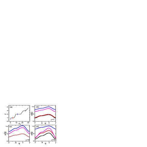
Figure 1: (Color online) Plots of the excitation energy $\omega(q)$ versus the wave number q (from $\Gamma$ to $X$, then $X$ to $T$, and finally $T$ to $\Gamma$, for a simple square lattice SCBZ ) for the BH model with two species of bosons. These plots show representative excitation spectra in the MI phases. (a) Total density $\rho$ versus $\mu_{a}$ for $U_{a}=11,~{}U_{b}=0.9U_{a},~{}\mu_{a}=\mu_{b}$ and $U_{ab}=0.6U_{a}$. The vertical lines in the Mott plateaux represent the $\mu_{a}$ values for which the excitation spectra were obtained for (b) $\rho=1$, (c) $\rho=2$, and (d) $\rho=3$, with all other parameters the same in all cases. For the MI phase with $\rho=1$, the excitation spectra consist of one-hole and three-particle excitations. In contrast, there are two- hole and particle excitations for $\rho=2$ and $3$. For the parameters chosen here, the lowest-energy excitation is degenerate for $\rho=2$.

III.1 RPA Excitation Spectra for the Bose-Hubbard Model with two species of bosons

The results of our RPA calculations for excitation spectra in the two-species BH model are shown by the representative plots in Figs.1 - 4. First we consider the excitation spectra in the MI phases, with total density of bosons $\rho=\rho_{a}+\rho_{b}=1$, $2$ and $3$, respectively, in Figs. 1 (b)-(d). We also plot $\rho$ versus $\mu_{a}$ for $U_{a}=11$, $U_{b}=0.9U_{a}$, $U_{ab}=0.6U_{a}$ and $\mu_{b}=\mu_{a}$ in Fig. 1(a) and mark, with vertical lines, the $\mu_{a}$ values for which the spectra was obtained in Figs. 1 (b)-(d). The excitation spectra in the MI phase with $\rho=1$, given in Fig. 1(b), show four excitations, one of which is a hole excitation and the rest are particle excitations (see Eq. (110) from Appendix for details). However, for $\rho=2$ and $\rho=3$, the spectra, plotted, respectively, in Figs. 1 (c) and (d), show four branches; these correspond to two-hole and two-particle excitations, which are the solutions of Eqs. 104 and 105. For $\rho=2$, two excitations are almost degenerate for the parameters we have considered. In all these cases we also obtain dispersionless modes, which are independent of ${\bf q}$ modes; we described these in the Appendix so we do not show them here.

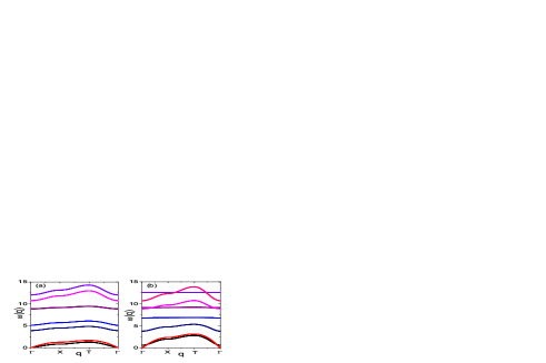
Figure 2: (Color online) Plots of excitation spectra (a) when both types of bosons are in the SF phase and (b) when only one type is in the SF and the other type of boson is in MI phase.

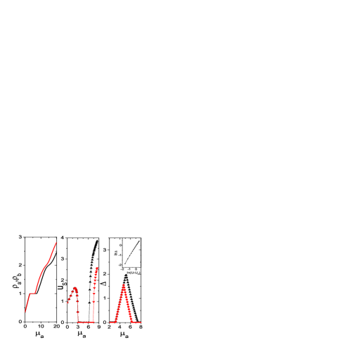
Figure 3: (Color online) (a) Plots of $\rho_{a}$ (red line) and $\rho_{b}$ (black line), for bosons of types $a$ and $b$, versus $\mu_{a}$ for $U_{a}=8,~{}U_{b}=0.9U_{a},~{}\mu_{a}=\mu_{b}$, and $U_{ab}=0.2U_{a}$; note the plateaux at integer values of $\rho_{a}$ and $\rho_{b}$. (b) The speed of sound $u_{s}$ versus $\rho_{a}$, for $U_{a}=8,~{}U_{b}=0.9U_{a},~{}\rho_{a}=\rho_{b}$, and $U_{ab}=0.2U$; $u_{s}$ is zero in the MI phase and finite in the SF phase. (c) The gap $\Delta$ versus $\mu_{a}$, for $U_{a}=8,~{}U_{b}=0.9U_{a},~{}\mu_{a}=\mu_{b}$ and $U_{ab}=0.2U_{a}$; the inset shows the power-law behavior of the gap in the vicinity of the transition at $U_{c}=3.1$.

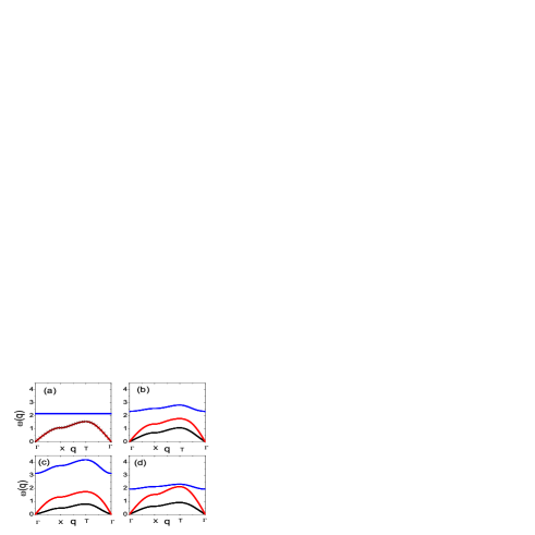
Figure 4: (Color online) Plots of the excitation energy $\omega(\bf{q})$ versus the wave number q for the BH model with two species of bosons, for $\rho=0.75,$ $U_{a}=9,~{}U_{b}=0.9U_{a}$, and (a) $U_{ab}=0.0$, (b) $U_{ab}=0.2U_{a}$, (c) $U_{ab}=0.4U_{a}$ and (d) $U_{ab}=-0.2U_{a}$.

The excitation spectra for the case where both $a$-type and $b$-type bosons are in the SF phase are given in the Fig. 2(a) which show two gapless excitations; linear in wave number near the point $\Gamma$ and excitations which have finite gap at the point $\Gamma$. Similarly, the excitation spectra for the case where only $b$-type bosons are in the SF phase and $a$-type bosons are in the MI phase are given in Fig. 2(b); we see only one gapless excitation corresponding to the SF phase of $b$-type bosons; and all the other branches of the excitation spectra have finite gaps at the point $\Gamma$. We also show some of the dispersionless spectra.

In Fig. 3 (a), we present plots versus $\mu_{a}=\mu_{b}$ of $\rho_{a}$ (red curve) and $\rho_{b}$ (black curve), for bosons of types $a$ and $b$, for $U_{a}=8,~{}U_{b}=0.9U_{a},~{}\mu_{a}=\mu_{b}$ and $U_{ab}=0.2U_{a}$, with plateaux at $\rho_{a}=1$ and/or $\rho_{b}=1$. In a gapless, SF phase, the speed of sound $u_{s}$ follows sheshadri55 from the slope of the excitation spectrum near the point $\Gamma$. In Fig. 3 (b), we show how the speed of sound $u_{s}$ behaves, for components $a$ (red dashed line) and $b$ (black dashed line with triangles), as functions of $\mu_{a}$, for the same parameters as in Fig. 3 (a); as we expect, $u_{s}$ is zero in the MI phases and positive in the SF phases.

From the excitation spectra we can obtain the gap $\Delta$ at the point $\Gamma$. In Fig. 3 (c), we show plots of $\Delta$ versus $\mu_{a}$ for the same parameters as in Figs. 3 (a) and (b); as we expect, $\Delta$ is zero in the SF phases (for bosons of types $a$ and $b$) and finite in the MI phases. In the inset of Fig. 3 (c) we shows that $\Delta$ approaches zero as $(U-U_{c})^{1/2}$, where $U_{c}$ is the critical value of $U$ at which the MI-SF transitions occur at these parameter values.

We now consider the first few low-energy excitation spectra in the SF phase; we hold $\rho=0.75$, but vary the $U_{ab}$ in Figs. 4 (a)-(c). In all these figures $U_{a}=9$, $U_{b}=0.9U_{a}$ and $\mu_{a}=\mu_{b}$. In Fig. 4 (a), $U_{ab}/U_{a}=0$, we see that the gapless mode is almost degenerate; and the next branch in the excitation spectrum is dispersionless; we do not show high-energy spectra here. As we increase $U_{ab}/U_{a}$, Fig. 4 (b) for $U_{ab}/U_{a}=0.2$ and Fig. 4 (c) for $U_{ab}/U_{a}=0.4$, the degeneracy of the gapless excitation spectrum is lifted and the spectra move away from each other. The non-dispersive mode now shows dispersion and moves to higher energies. In Fig. 4 (d), we illustrate the excitation spectra for $U_{ab}/U_{a}<0$; we see again that the gapless modes move away from each other; and we observe that the excitation frequencies of other modes are different compared to their values for $U_{ab}/U_{a}>0$. Our results are qualitatively similar to those of the Gutzwiller-based, excitation-spectrum study of Ref. ozaki0955 , which presents $k_{x}=k_{y}$ scans through the reciprocal lattice of a two-dimensional square lattice.

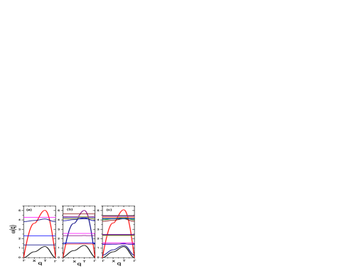
Figure 5: (Color online) Plots of the excitation energy $\omega$ versus the wave number q for the spin-1 BH model: (a) superfluid ($U_{0}=2,~{}\mu=5$ and $~{}U_{2}/U_{0}=0$), (b) polar-superfluid ($U_{0}=2,~{}\mu=5$ and $~{}U_{2}/U_{0}=0.03$) and (c) ferromagnetic-superfluid ($U_{0}=2,~{}\mu=5$ and $U_{2}/U_{0}=-0.03$) phases. In (a) and (b) the lowest modes are two gapless, degenerate modes, shown in black, whose energy approaches zero quadratically at small wave numbers q (near $\Gamma$). In (c) we see clearly the splitting of the degenerate modes, which now have a gap and then a quadratic dependence on q near $\Gamma$. In all three cases, there is another mode, shown in red, whose energy goes to zero linearly at small q. All the higher excitations have finite gaps at $\Gamma$ and are highly degenerate. The degeneracies of these modes are partially lifted in the case of polar and ferromagnetic SF phases.

III.2 RPA Excitation Spectra for the Spin-1 Bose-Hubbard Model

We now give representative plots of our RPA excitation spectra for the spin-1 BH model, in Figs. 5 (a)-(c) for $~{}U_{2}/U_{0}=0$, $~{}U_{2}/U_{0}=0.03$, and $U_{2}/U_{0}=-0.03$, which yield, respectively, a pure SF with no spin interactions, a polar SF, and a ferromagnetic SF for the parameter values given in the figure caption rvpspin155 . The excitation spectra are qualitatively different in these three cases. In the SF (Fig. 5 (a)) phase there are two gapless, degenerate modes, shown in black, whose frequencies approach zero quadratically at small wave numbers q (near $\Gamma$); there is another mode, shown in red, whose energy goes to zero linearly at small q. All the other excitations spectra have finite gap at $\Gamma$; some of these spectra are degenerate and some are ${\bf q}$ independent; e.g., the spectra shown in green, blue, and maroon are ${\bf q}$ independent and have degeneracies 3, 4, and 8, respectively. The branch shown in navy blue is weakly q dependent and is doubly degenerate. These degeneracies are partially lifted when $U_{2}$ is finite. In the polar SF (Fig. 5 (b)), the lowest modes, shown in black, are doubly degenerate and have a quadratic dependence on q as in the case of a pure SF. However, the next branch, which displays a linear dependence on q near the $\Gamma$ point, as in the case of a pure SF, becomes approximately dispersionless at higher value of q, and avoids level crossing with the branch shown in green (these acquire a ${\bf q}$ dependence). Note that this spectrum, dispersionless and with a triple degeneracy in the pure SF case, has its degeneracy lifted partially: the spectrum shown in navy blue is non-degenerate and the one shown in blue is doubly degenerate; we obtain similar behaviors in higher-energy excitation spectra. In the ferromagnetic SF (Fig. 5 (c)), we see clearly the splitting of the degenerate modes, which now have a gap and then a quadratic dependence on q near $\Gamma$; the red curve indicates the gapless mode, which approaches $\Gamma$ linearly. The degeneracies of higher modes are also lifted in this case. The qualitative features of these spectra agree with those found for the various SF phases in the spin-1, Gross-Pitaevskii study of Ref. tlho55 .

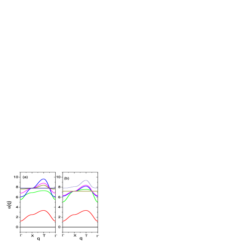
Figure 6: (Color online) Plots of the excitation frequency $\omega({\bf q})$ versus the wave number q for the spin-1 BH model in the MI1 phase with $\rho=1$: (a) $U_{0}=10$, $\mu=2.5$ and $U_{2}/U_{0}=0.03$ and (b) $U_{0}=10$, $\mu=2.5$ and $U_{2}/U_{0}=-0.03$. The MI1 ground state is degenerate; and these excited states do not couple to the ground state through particle or hole excitations; this gives the the dispersionless mode at $\omega(\bf{q})=0$. The mode shown in red is a hole excitation; all the higher-energy modes shown are particle excitations.

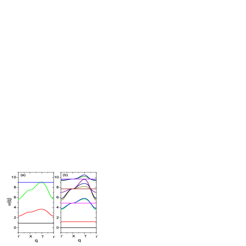
Figure 7: (Color online) Plots of the excitation energy $\omega(\bf{q})$ versus the wave number q for the spin-1 BH model with $\rho=2$: (a) $U_{0}=10,~{}\mu=12.5$ and $~{}U_{2}/U_{0}=0.03$ and (b) $U_{0}=13,~{}\mu=17.5$ and $U_{2}/U_{0}=-0.03$.

Figure 8: The sound speed $u_{s}$ versus $U_{0}$ in the vicinity of the polar-SF-MI2 transition for $\mu=10$ and $U_{2}/U_{0}=0.03$, with $(\rho=2)$; $u_{s}$ jumps to zero at this first-order transition; by contrast, (see inset for $~{}\mu=5$ and $U_{2}/U_{0}=0.03$) $u_{s}$ goes to zero continuously at the SF-MI1 transition.

We present excitation spectra in the MI1 and MI2 phases in Figs. 6 and  7, respectively. Here, MI1 and MI2 denote, respectively, Mott phases with one and two bosons per site. For MI1, we obtain qualitatively similar excitation spectra for $U_{2}/U_{0}>0$ (Figs. 6(a)) and $U_{2}/U_{0}<0$ (Figs. 6(b)). For $U_{2}/U_{0}>0$, the ground state for MI1 is triply degenerate (Appendix); these degenerate states do not couple to each other through the creation of a particle or hole. Thus, the lowest excitation, $\omega({\bf q})=0$, represented in black in Fig. 6(a), is doubly degenerate and dispersionless. The non-degenerate hole excitation is shown in red. The excitations, above the hole excitation, are six-particle excitations, two of which are dispersionless and degenerate. We find similar excitation spectra for $U_{2}/U_{0}<0$ (Figs. 6(b)).

For MI2, we obtain qualitatively different excitation spectra for $U_{2}/U_{0}>0$ (Figs. 7(a)) and $U_{2}/U_{0}<0$ (Figs. 7(b)). For $U_{2}/U_{0}>0$, the MI2 ground state is non-degenerate (Appendix) because of the formation of a singlet, so there is no dispersionless mode with $\omega(\bf{q})=0$. The first excited state of our MFT hamiltonian (Eq. 11) has five-fold degeneracy; and the ground state does not couple to these states via particle or hole excitations. This gives us the dispersionless mode (black line). The dispersive mode with the lowest energy comprises hole excitations (red curves); this mode is triply degenerate. The particle excitations are also dispersive (green curve, degeneracy 3), except for the one shown in blue (degeneracy 6). Higher-energy excitations are multi-particle-hole excitations and are dispersionless; we do not show these here.

In Fig. 8 we plot the sound speed $u_{s}$ versus $U_{0}$ in the vicinity of the polar-SF-MI2 transition for $\mu=10$ and $U_{2}/U_{0}=0.03$, with $(\rho=2)$; $u_{s}$ jumps to zero at this first-order transition; by contrast, (see inset for $~{}\mu=5$ and $U_{2}/U_{0}=0.03$) $u_{s}$ goes to zero continuously at the phase-SF-MI1 transition. The natures of these transitions are consistent with the predictions of the mean-field theory rvpspin155 on which we base our RPA study.

We do not investigate magnetic ordering and magnetic excitations in the MI phase of the spin-1 model because, as has been noted earlier, our mean-field theory does not allow for any magnetic structure in the MI phase in this model rvpspin155 .

III.3 RPA Excitation Spectra for the Extended Bose-Hubbard model

We now show representative RPA excitation spectra in Figs. 9 (a), (b), (c), (d), and (e) for SF, DW $3/2$ (see Ref. JMK12 ), SS , MI1, and DW $1/2$ phases for $V=0.6U$ and (a) $U=6,~{}\mu=11.3$, (b) $U=10,~{}\mu=19$, (c) $U=8.3,~{}\mu=15.4$, (d) $U=12,~{}\mu=10$, and (e) $U=12,~{}\mu=5$. By the symbol DW $n/m$, we mean a density-wave phase with $n$ bosons per site and $m$ sites per unit cell. From these excitation spectra we obtain $u_{s}$, whose dependence on $U$ is shown in Fig. 9 (f), as the system moves from the SF to the SS phase and then to the DW $3/2$ phase, for $V=0.6U$, and $\rho_{total}=3$; the sharp drop in $u_{s}$ at the SS-DW $3/2$ boundary indicates a first-order transition; the inset shows that $u_{s}\sim\sqrt{U}$ in the small-$U$ regime in the SF phase.

The RPA excitation spectra have a gap at the $\Gamma$ point when the system is in the DW 3/2 phase and this gap $\Delta$ goes to zero as the system approaches the SS phase. In Fig. 10 $(a)$ we plot $\Delta$ versus $U$ as the system goes from the DW to the SS phase. Figure 10 $(b)$ show analogous plots for the SF-MI transition. The behaviors of this gap are what we expect on general grounds, i.e., it jumps discontinuosly to zero at the DW $3/2$ to SS transition, but it goes to zero continuously, as $\Delta\sim(U-U_{c})^{1/2}$, at the MI1 to SF transition at the critical value $U_{c}$. This exponent of $1/2$ is a mean-field exponent, which should be modified by fluctuations (this MI1-SF transition lies in the $d$-dimensional XY universality class).

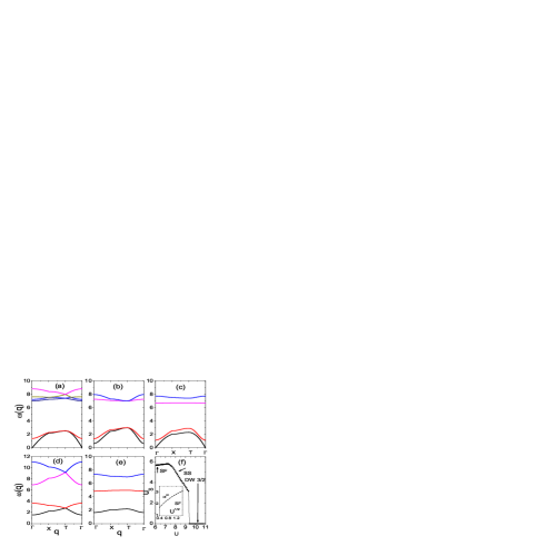
Figure 9: (Color online) Plots of the excitation frequency $\omega(\bf{q})$ versus the wave number q for the EBH model in (a) $U=6,~{}V=0.6U,~{}\mu=11.3$, and $\rho_{total}=3$, (b) $U=10,~{}V=0.6U,~{}\mu=19,~{}\rho_{total}=3$, (c) $U=8.3,~{}V=0.6U,~{}\mu=15.4,~{}\rho_{total}=3$, (d) $U=12,~{}V=0.6U,~{}\mu=10,~{}\rho_{total}=2$, and (e) $U=12,~{}V=0.6U,~{}\mu=5,~{}\rho_{total}=1$. We show the excitation spectra in the SF, DW3/2, SS, MI1, and DW1/2 phases, respectively. In (f) $V=0.6U,~{}\rho_{total}=3$; and we show the dependence of $u_{s}$ on $U$ as the system goes from the SF to the SS and then to the DW3/2 phase; the last transition is clearly first order; the inset shows the $u_{s}\sim\sqrt{U}$ behavior at low $U$ in the SF phase.

Figure 10: Plots of the gap $\Delta$ in the RPA excitation spectrum as a function of $U$ (a) near the SS-DW3/2 transition and $(b)$ near the SF-MI transition; the inset shows the power-law behavior of the gap in the vicinity of the transition at $U_{c}=5.7$.

IV Conclusions

We have obtained representative excitation spectra in all phases of three generalized Bose-Hubbard (BH) models, namely, (1) a two-species generalization of the spinless BH model, (2) a spin-1 BH model, and (3) the extended Bose-Hubbard model (EBH) for spinless interacting bosons of one species. Our study uses the random phase approximation (RPA), which it develops, in a unified way, by starting from mean-field theories of the type that we have discussed in Ref. rvpspin155 . Thus, it generalizes the RPA studies initiated in Ref. sheshadri55 for the simple BH model and continued, e.g., in Refs. Konabe55 ; Menotti ; iskin09 .

Our study yields a variety of interesting results that we have described in detail in the previous Section. In particular, our RPA excitation spectra show clear gaps in MI phases, in all the models above, in the DW phases in the EBH model, and gapless spectra in all SF phases and the SS phase in the EBH model. From these spectra we have obtained the dependence of (a) gaps $\Delta$ and (b) the sound velocity $u_{s}$ on the parameters of these models. We have also investigated the behaviors of $\Delta$ and $u_{s}$ as these systems go through phase transitions. We find that, at the polar SF-MI transitions in the spin-1 BH model, $u_{s}$ goes to zero continuously (discontinuously) for MI phases with an odd (even) number of bosons per site; this is consistent with the natures of these transition (continuous or discontinuous) in the mean-field theory for the spin-1 BH model rvpspin155 .

In the SF phases of these models, our excitation spectra agree qualitatively, at weak couplings, with those that can be obtained from Gross-Pitaevskii-type models. For example, our RPA excitation spectra are qualitatively similar to those obtained for ferromagnetic and polar superfluids in tlho55 , which uses a spin-1 generalization of the Gross-Pitaevskii equation.

Excitation spectra, at the level of the RPA, can also be obtained by starting with a Gutzwiller-type mean-field theory. Such studies, carried out, e.g., for two-boson BH models, the spin-1 BH models, and the EBH model, should be formally equivalent to our RPA study; however, we are not aware of any study that has shown this in complete detail. We do not know of one, unified treatment of Gutzwiller-type RPA, like our unified RPA study for these three models, so a direct comparison of our results with these Gutzwiller-type studies is not completely straightforward. Reference Hou has evaluated the excitation spectrum of spin-1 bosonic atoms in a Mott-insulator phase. Hou, et al. have investigated the quantum phase transition of spin-2 cold bosons in an optical lattice with and without an external magnetic field, Hou2 ; they also obtain Gutzwiller-type RPA excitation spectra.

Previous studies have analyzed excitation spectra in the two-species BH model. In the MI phase, the lowest two branches of the excitation spectrum have gaps; and they correspond to the particle- and hole-excitation modes Elstner55 ; Oosten55 ; Altman55 ; Konabe55 . In the SF phase, the excitation spectrum has one gapless mode and one mode with a gap E.Altman55 ; Huber55 ; Krutitsky55 ; Podolsky55 ; Pollet55 ; the gapless mode arises because of oscillations of the phase of the SF order parameter (this is the Bogoliubov mode); the lowest mode with the gap arises because of the amplitude mode in the vicinity of the SF-MI transition at integer fillings; this amplitude mode becomes gapless at the critical point. Our study explores the dependence of the excitation spectra on model parameters in far greater detail than earlier studies.

Furthermore, the RPA method can be used to obtain the complete $\omega$ and $\bf{q}$ dependence of the Green function as noted, e.g., in Refs. Konabe55 ; Menotti for the simple, spinless BH model. From this, various properties can be calculated, e.g., the momentum distribution function; the latter has been obtained in the RPA in iskin09 for the EBH model. We give a brief description of such Green-function studies in the Appendix and their generalzations for the three models we consider here.

Excitation spectra have been measured experimentally by Bragg-spectroscopy Stenger55 ; Steinhauer55 ; Ernst55 ; Clement55 ; Bissbort55 ; Miyake55 ; Fabbri55 and lattice-amplitude-modulation Stoerle55 ; Schori55 ; Endres55 methods; and these measurements have been used to characterize SF and MI phases and the transition between them. We hope our work will lead to experimental measurements of the spectra of elementary excitations in the different phases in the physical realizations of the generalized BH models we have discussed above. Momentum-distribution functions can be calculated, at the RPA level, from the Green functions that we have obtained. The calculation is especially simple in a Mott phase, as illustrated, e.g., in Ref. iskin09 . Such momentum-distribution functions can be compared with those that are measured experimentally as discussed, e.g., in Refs. rmp55 ; iskin09 . The studies of Refs. Menotti ; iskin09 also mention some of the limitations of the RPA in the context of the BH model; e.g., Ref. Menotti notes that this type of of RPA, when applied to the simple BH model, yields a violation of the total density sum rule.

Excitation spectra can also be measured by Quantum Monte Carlo (QMC) simulation as shown for the simple BH model in Ref. mc55 and a continuation model in Ref. Saccani . We hope our study will lead to QMC studies of the excitation spectral of the generalized BH models we have discussed here.

V Acknowledgments

We thank DST, UGC, CSIR (India)(No. 03(1306)/14/EMR-II) for support and K. Sheshadri for useful discussions. JMK and RVP thank, respectively, the University of Goa and the Indian Institute of Science, for hospitality during the period in which this paper was being written.

Appendix A The Random-Phase Approximation.

We illustrate below how we obtain the RPA equations for the Green functions for our Bose-Hubbard (BH) models of Eqs. (1), (2), and (3), respectively.

The RPA equation of motion, for any of these BH models use the operators $L_{\alpha\alpha^{\prime}}^{i}=|i\alpha\rangle\langle i\alpha^{\prime}|$, where $|i\alpha\rangle$ is the eigenvector for the mean-field Hamiltonian for site $i$. Any single-site operator can be expressed as $\hat{O}\equiv\sum_{i\alpha\alpha^{\prime}}\langle i\alpha|\hat{O}|i\alpha^{\prime}\rangle L_{\alpha\alpha^{\prime}}^{i}$, so the Hamiltonian for these BH models can be written as

$${\cal{H}}^{m}= -\sum_{i\alpha\alpha^{\prime}}V^{i,m}_{\alpha\alpha^{\prime}}L^{i,m}_{\alpha\alpha^{\prime}}-\sum_{ij,\alpha\alpha^{\prime},\beta\beta^{\prime}}T^{ij,m}_{\alpha\alpha^{\prime},\beta\beta^{\prime}}L^{i,m}_{\alpha\alpha^{\prime}}L^{j,m}_{\beta\beta^{\prime}},$$

where the superscript $m=1$, is for two species of bosons, $m=2$ is for the spin-1 BH model, and $m=3$ is for the EBH model.

$$V^{i,1}_{\alpha\alpha^{\prime}}= (\mu_{a}+\frac{U_{a}}{2})\langle i\alpha|\hat{n}_{a}|i\alpha^{\prime}\rangle-\frac{U_{a}}{2}\langle i\alpha|\hat{n}_{a}^{2}|i\alpha^{\prime}\rangle$$ (35)

$$+(\mu_{b}+\frac{U_{b}}{2})\langle i\alpha|\hat{n}_{b}|i\alpha^{\prime}\rangle-\frac{U_{b}}{2}\langle i\alpha|\hat{n}_{b}^{2}|i\alpha^{\prime}\rangle$$

$$-U_{ab}\langle i\alpha|\hat{n}_{a}\hat{n}_{b}|i\alpha^{\prime}\rangle,$$

$$V^{i,2}_{\alpha\alpha^{\prime}} = (\mu+\frac{U_{0}}{2})\langle i\alpha|\hat{n}_{i}|i\alpha^{\prime}\rangle-\frac{U_{0}}{2}\langle i\alpha|\hat{n}_{i}^{2}|i\alpha^{\prime}\rangle$$ (36)

$$-\frac{U_{2}}{2}\langle i\alpha|(\vec{F}^{2}_{i}-2\hat{n}_{i})|i\alpha^{\prime}\rangle,$$

$$V^{i,3}_{\alpha\alpha^{\prime}}=(\mu+\frac{U}{2})\langle i\alpha|\hat{n}_{i}|i\alpha^{\prime}\rangle-\frac{U}{2}\langle i\alpha|\hat{n}_{i}^{2}|i\alpha^{\prime}\rangle,$$ (37)

and

$$T^{ij,1}_{\alpha\alpha^{\prime},\beta\beta^{\prime}}=\langle i\alpha|\hat{a}_{i}^{\dagger}|i\alpha^{\prime}\rangle\langle j\beta|\hat{a}_{j}|j\beta^{\prime}\rangle+\langle i\alpha|\hat{a}_{i}|i\alpha^{\prime}\rangle\langle j\beta|\hat{a}_{j}^{\dagger}|j\beta^{\prime}\rangle+\langle i\alpha|\hat{b}_{i}^{\dagger}|i\alpha^{\prime}\rangle\langle j\beta|\hat{b}_{j}|j\beta^{\prime}\rangle+\langle i\alpha|\hat{b}_{i}|i\alpha^{\prime}\rangle\langle j\beta|\hat{b}_{j}^{\dagger}|j\beta^{\prime}\rangle,$$ (38)

$$T^{ij,2}_{\alpha\alpha^{\prime},\beta\beta^{\prime}}=\sum_{\sigma}\{\langle i\alpha|\hat{a}_{i,\sigma}^{\dagger}|i\alpha^{\prime}\rangle\langle j\beta|\hat{a}_{j,\sigma}|j\beta^{\prime}\rangle+\langle i\alpha|\hat{a}_{i,\sigma}|i\alpha^{\prime}\rangle\langle j\beta|\hat{a}_{j,\sigma}^{\dagger}|j\beta^{\prime}\rangle\},$$ (39)

$$T^{ij,3}_{\alpha\alpha^{\prime},\beta\beta^{\prime}}=\langle i\alpha|\hat{a}_{i}^{\dagger}|i\alpha^{\prime}\rangle\langle j\beta|\hat{a}_{j}|j\beta^{\prime}\rangle+\langle i\alpha|\hat{a}_{i}|i\alpha^{\prime}\rangle\langle j\beta|\hat{a}_{j}^{\dagger}|j\beta^{\prime}\rangle-V\langle i\alpha|\hat{n}_{i}|i\alpha^{\prime}\rangle\langle j\beta|\hat{n}_{j}|j\beta^{\prime}\rangle.$$ (40)

The propagator $G^{ij,m}_{\alpha\alpha^{\prime},\beta\beta^{\prime}}(t,t^{\prime})$, is the amplitude for the $j^{th}$ site to flip between the states $\beta$ and $\beta^{\prime}$ at $t^{\prime}$, given that the $i^{th}$ site has flipped between states $\alpha$ and $\alpha^{\prime}$ at $t$. We have

$$G^{ij,m}_{\alpha\alpha^{\prime},\beta\beta^{\prime}}(t,t^{\prime}) = -i\theta(t-t^{\prime})\langle[L^{i,m}_{\alpha\alpha^{\prime}}(t),L^{j,m}_{\beta\beta^{\prime}}(t^{\prime})]\rangle$$ (41)

$$= \langle\langle L^{i,m}_{\alpha\alpha^{\prime}}(t)|L^{j,m}_{\beta\beta^{\prime}}(t^{\prime})\rangle\rangle.$$

The equation of motion for this Green function, with $t^{\prime}=0$, is calculated as follows:

$$\frac{d}{dt}G^{ij,m}_{\alpha\alpha^{\prime},\beta\beta^{\prime}}(t) = -i\frac{d\theta(t)}{dt}\langle\left[L^{i,m}_{\alpha\alpha^{\prime}}(t),L^{j,m}_{\beta\beta^{\prime}}(0)\right]\rangle$$ (42)

$$-i\theta(t)\frac{d}{dt}\langle\left[L^{i,m}_{\alpha\alpha^{\prime}}(t),L^{j,m}_{\beta\beta^{\prime}}(0)\right]\rangle,$$

where

$$\frac{d}{dt}L^{i,m}_{\alpha\alpha^{\prime}}(t)=\frac{1}{i\hbar}\left[{\cal{H}}^{m},L^{i,m}_{\alpha\alpha^{\prime}}(t)\right]\equiv i\left[L^{i,m}_{\alpha\alpha^{\prime}}(t),{\cal{H}}^{m}\right]$$

we have set $\hbar=1$, and we obtain the second term on the right-hand side of Eq. (42)

$$-i\frac{d}{dt} \left[L^{i,m}_{\alpha\alpha^{\prime}}(t),L^{j,m}_{\beta\beta^{\prime}}(0)\right]=\left[L^{i,m}_{\alpha\alpha^{\prime}}(t),{\cal{H}}^{m}\right]L^{j,m}_{\beta\beta^{\prime}}(0)$$ (44)

$$-L^{j,m}_{\beta\beta^{\prime}}(0)\left[L^{i,m}_{\alpha\alpha^{\prime}}(t),{\cal{H}}^{m}\right]$$

By using Eq. (A) in the above equation, substituting it in Eq. (42) and carrying out the RPA, where we replace thermal averages of products of operators by the products of their thermal averages, to obtain

$$\frac{d}{dt}G^{ij,m}_{\alpha\alpha^{\prime},\beta\beta^{\prime}}(t)=-i\delta(t)\delta_{\alpha^{\prime}\beta}\delta_{\alpha\beta^{\prime}}{P}^{m}_{\alpha\alpha^{\prime}}+i({\omega}^{m}_{\alpha^{\prime}}-{\omega}^{m}_{\alpha})G^{ij,m}_{\alpha\alpha^{\prime},\beta\beta^{\prime}}(t)+i{P}^{m}_{\alpha\alpha^{\prime}}\sum_{l}\sum_{\mu\nu}T^{il,m}_{\alpha\alpha^{\prime},\nu\mu}G^{lj,m}_{\mu\nu,\beta\beta^{\prime}}(t).$$ (45)

Fourier transformation over space and time for $m=1$ and $m=2$ now yields

$$(\omega-{\omega}^{m}_{\alpha}+{\omega}^{m}_{\alpha^{\prime}})G^{m}_{\alpha\alpha^{\prime},\beta\beta^{\prime}}(\mathbf{q},\omega)+{P}^{m}_{\alpha\alpha^{\prime}}\sum_{\mu\nu}T^{m}_{\alpha\alpha^{\prime},\nu\mu}(\mathbf{q})G^{m}_{\mu\nu,\beta\beta^{\prime}}\mathbf{q},\omega)=\frac{1}{2\pi}{P}^{m}_{\alpha\alpha^{\prime}}\delta_{\alpha\beta^{\prime}}\delta_{\beta\alpha^{\prime}};$$ (46)

and, for $m=3$ with a bipartite hypercubic lattice, with two sublattices ${\mathcal{A}}$ and ${\mathcal{B}}$, we get

$$(\omega-{\omega}^{m}_{\alpha}+{\omega}^{m}_{\alpha^{\prime}}){G}^{AA}_{\alpha\alpha^{\prime},\beta\beta^{\prime}}(\mathbf{q},\omega)+{P}^{m}_{\alpha\alpha^{\prime}}\sum_{\mu\nu}T^{m}_{\alpha\alpha^{\prime},\nu\mu}(\mathbf{q})G^{BA}_{\mu\nu,\beta\beta^{\prime}}(\mathbf{q},\omega)=\frac{1}{2\pi}{P}^{m}_{\alpha\alpha^{\prime}}\delta_{\alpha\beta^{\prime}}\delta_{\beta\alpha^{\prime}},$$ (47)

$$(\omega-{\omega}^{m}_{\alpha}+{\omega}^{m}_{\alpha^{\prime}}){G}^{BA}_{\alpha\alpha^{\prime},\beta\beta^{\prime}}(\mathbf{q},\omega)+P^{m}_{\alpha\alpha^{\prime}}\sum_{\mu\nu}T^{m}_{\alpha\alpha^{\prime},\nu\mu}(\mathbf{q})G^{AA}_{\mu\nu,\beta\beta^{\prime}}(\mathbf{q},\omega)=0,$$ (48)

where $T^{m}_{\alpha\alpha^{\prime},\beta\beta^{\prime}}(\textbf{q})=\epsilon_{\textbf{q}}(T^{ij,m}_{\alpha\alpha^{\prime},\beta\beta^{\prime}}+T^{ji,m}_{\beta\beta^{\prime},\alpha\alpha^{\prime}})$, $\epsilon_{q}\equiv-2t\sum_{j=x,y}cos(q_{j})$, ${P}^{m}_{\alpha\alpha^{\prime}}=\langle{L}^{m}_{\alpha\alpha}\rangle-\langle{L}^{m}_{\alpha^{\prime}\alpha^{\prime}}\rangle$ and ${\omega}^{m}_{\alpha}={V}^{m}_{\alpha\alpha}+\sum_{\beta}{T}^{m}_{\alpha\alpha,\beta\beta}(q=0)\langle{L}^{m}_{\beta\beta}\rangle$, and $\omega$ and $\mathbf{q}$ are, respectively, the frequency and wave vector of the excitation. The poles of these Green functions give the different branches of the excitation spectrum in the RPA.

We can relate the Green functions calculated above to the single-particle Green function $g_{i,j}(t)=-i\theta(t)\langle[\hat{a}_{i}(t),\hat{a}^{\dagger}_{j}]\rangle$. We first illustrate this for the simple BH model by following the treatment of Ref. Matsumoto . We define the single-particle Green functions

$$g_{1}(\textbf{q},\omega) = \sum_{\alpha\alpha^{\prime},~{}\beta\beta^{\prime}}y^{\dagger}_{\alpha,\alpha^{\prime}}~{}y_{\beta,\beta^{\prime}}G_{\alpha\alpha^{\prime},\beta\beta^{\prime}}(\textbf{q},\omega),$$ (49)

$$g_{2}(\textbf{q},\omega) = \sum_{\alpha\alpha^{\prime},~{}\beta\beta^{\prime}}y^{\dagger}_{\alpha,\alpha^{\prime}}~{}y^{\dagger}_{\beta,\beta^{\prime}}G_{\alpha\alpha^{\prime},\beta\beta^{\prime}}(\textbf{q},\omega),$$ (50)

where ${y_{\alpha,\alpha^{\prime}}~{}\equiv~{}\langle i,\alpha|\hat{a}_{i}|i,\alpha^{\prime}\rangle}$ and ${y^{\dagger}_{\alpha,\alpha^{\prime}}~{}\equiv~{}\langle i,\alpha|\hat{a}^{\dagger}_{i}|i,\alpha^{\prime}\rangle}$ are independent of the position $i$. It is easy to show that equation of motion for the green functions $g_{1}(\textbf{q},\omega)$ and $g_{2}(\textbf{q},\omega)$ can be written as

$$\left(\begin{array}[]{cccccccc}\mbox{${1-\epsilon_{q}A_{11}}$}&\mbox{${\epsilon_{q}A_{12}}$}\\ \mbox{${\epsilon_{q}A_{21}}$}&\mbox{${1-\epsilon_{q}A_{22}}$}\\ \end{array}\right)~{}\left(\begin{array}[]{cccccccc}\mbox{${g_{1}(q,\omega)}$}\\ \mbox{${g_{2}(q,\omega)}$}\\ \end{array}\right)~{}=~{}\left(\begin{array}[]{cccccccc}\mbox{${A_{11}}$}\\ \mbox{${A_{21}}$}\\ \end{array}\right),$$ (57)

where

$$\left(\begin{array}[]{cccccccc}\mbox{${A_{11}}$}&\mbox{${A_{12}}$}\\ \mbox{${A_{21}}$}&\mbox{${A_{22}}$}\\ \end{array}\right)~{}=~{}\sum_{\alpha}\frac{\left(\begin{array}[]{cccccccc}\mbox{${{y}_{0,\alpha}{y}^{\dagger}_{\alpha,0}}$}&\mbox{${{y}_{0,\alpha}{y}_{\alpha,0}}$}\\ \mbox{${{y}^{\dagger}_{0,\alpha}{y}^{\dagger}_{\alpha,0}}$}&\mbox{${{y}^{\dagger}_{0,\alpha}{y}_{\alpha,0}}$}\\ \end{array}\right)}{\omega+i\delta+(\omega_{0}-\omega_{\alpha})}~{}-~{}\sum_{\alpha}\frac{\left(\begin{array}[]{cccccccc}\mbox{${{y}^{\dagger}_{0,\alpha}{y}_{\alpha,0}}$}&\mbox{${{y}_{0,\alpha}{y}_{\alpha,0}}$}\\ \mbox{${{y}^{\dagger}_{0,\alpha}{y}^{\dagger}_{\alpha,0}}$}&\mbox{${{y}_{0,\alpha}{y}^{\dagger}_{\alpha,0}}$}\\ \end{array}\right)}{\omega+i\delta+(\omega_{\alpha}-\omega_{0})},$$ (64)

$|0\rangle$ represents the ground state and the summation is over all the excited states $\alpha$.

We give below the analogs of Eqs.(57)-(64) for the BH model with two species of bosons in Eqs.(79) and (92) and for the spin-1 BH model in Eq.(93). For $a$-type bosons, we define the single-particle Green functions

$$g^{MN}_{1}(\textbf{q},\omega) = \sum_{\alpha\alpha^{\prime},~{}\beta\beta^{\prime}}{y^{\dagger}}^{M}_{\alpha,\alpha^{\prime}}~{}y^{N}_{\beta,\beta^{\prime}}G_{\alpha\alpha^{\prime},\beta\beta^{\prime}}(\textbf{q},\omega),$$

$$g^{MN}_{2}(\textbf{q},\omega) = \sum_{\alpha\alpha^{\prime},~{}\beta\beta^{\prime}}{y^{\dagger}}^{M}_{\alpha,\alpha^{\prime}}~{}{y^{\dagger}}^{N}_{\beta,\beta^{\prime}}G_{\alpha\alpha^{\prime},\beta\beta^{\prime}}(\textbf{q},\omega),$$

where the superscripts $M$ and $N$ can be $a$ or $b$, for the two-species BH model, or $\sigma$ and $\sigma^{\prime}$ for the spin-1 BH model. For the two-species BH model, the equation of motion for the Green functions $g^{MN}_{1}(\textbf{q},\omega)$ and $g^{MN}_{2}(\textbf{q},\omega)$ can be written as

$$\left(\begin{array}[]{cccccccc}\mbox{${1-\epsilon_{p}A^{aa}_{11}}$}&\mbox{${\epsilon_{p}A^{ba}_{11}}$}&\mbox{${\epsilon_{p}A^{aa}_{12}}$}&\mbox{${\epsilon_{p}A^{ba}_{12}}$}\\ \mbox{${\epsilon_{p}A^{ab}_{11}}$}&\mbox{${1-\epsilon_{p}A^{bb}_{11}}$}&\mbox{${\epsilon_{p}A^{ab}_{12}}$}&\mbox{${\epsilon_{p}A^{bb}_{12}}$}\\ \mbox{${\epsilon_{p}A^{aa}_{21}}$}&\mbox{${\epsilon_{p}A^{ba}_{21}}$}&\mbox{${1-\epsilon_{p}A^{aa}_{22}}$}&\mbox{${\epsilon_{p}A^{ba}_{22}}$}\\ \mbox{${\epsilon_{p}A^{ab}_{21}}$}&\mbox{${\epsilon_{p}A^{bb}_{21}}$}&\mbox{${\epsilon_{p}A^{ab}_{22}}$}&\mbox{${1-\epsilon_{p}A^{bb}_{22}}$}\end{array}\right)~{}\left(\begin{array}[]{cccccccc}\mbox{${g^{aa}_{1}(q,\omega)}$}\\ \mbox{${g^{ba}_{1}(q,\omega)}$}\\ \mbox{${g^{aa}_{2}(q,\omega)}$}\\ \mbox{${g^{ba}_{2}(q,\omega)}$}\\ \end{array}\right)~{}=~{}\left(\begin{array}[]{cccccccc}\mbox{${A^{aa}_{11}}$}\\ \mbox{${A^{ab}_{11}}$}\\ \mbox{${A^{aa}_{21}}$}\\ \mbox{${A^{ab}_{21}}$}\\ \end{array}\right),$$ (79)

$$\left(\begin{array}[]{cccccccc}\mbox{${1-\epsilon_{p}A^{bb}_{11}}$}&\mbox{${\epsilon_{p}A^{ab}_{11}}$}&\mbox{${\epsilon_{p}A^{bb}_{12}}$}&\mbox{${\epsilon_{p}A^{ab}_{12}}$}\\ \mbox{${\epsilon_{p}A^{ba}_{11}}$}&\mbox{${1-\epsilon_{p}A^{aa}_{11}}$}&\mbox{${\epsilon_{p}A^{ba}_{12}}$}&\mbox{${\epsilon_{p}A^{aa}_{12}}$}\\ \mbox{${\epsilon_{p}A^{bb}_{21}}$}&\mbox{${\epsilon_{p}A^{ab}_{21}}$}&\mbox{${1-\epsilon_{p}A^{bb}_{22}}$}&\mbox{${\epsilon_{p}A^{ab}_{22}}$}\\ \mbox{${\epsilon_{p}A^{ba}_{21}}$}&\mbox{${\epsilon_{p}A^{aa}_{21}}$}&\mbox{${\epsilon_{p}A^{ba}_{22}}$}&\mbox{${1-\epsilon_{p}A^{aa}_{22}}$}\end{array}\right)~{}\left(\begin{array}[]{cccccccc}\mbox{${g^{bb}_{1}(q,\omega)}$}\\ \mbox{${g^{ab}_{1}(q,\omega)}$}\\ \mbox{${g^{bb}_{2}(q,\omega)}$}\\ \mbox{${g^{ab}_{2}(q,\omega)}$}\\ \end{array}\right)~{}=~{}\left(\begin{array}[]{cccccccc}\mbox{${A^{bb}_{11}}$}\\ \mbox{${A^{ba}_{11}}$}\\ \mbox{${A^{bb}_{21}}$}\\ \mbox{${A^{ba}_{21}}$}\\ \end{array}\right).$$ (92)

For the spin-1 BH model we have:

$$\left(\begin{array}[]{cccccccc}\mbox{${1-\epsilon_{p}A^{\sigma\sigma}_{11}}$}&\mbox{${\epsilon_{p}\sum_{\sigma^{\prime}}A^{\sigma\sigma^{\prime}}_{12}}$}\\ \mbox{${\epsilon_{p}A^{\sigma^{\prime}\sigma}_{21}}$}&\mbox{${1-\epsilon_{p}A^{\sigma^{\prime}\sigma^{\prime}}_{22}}$}\\ \end{array}\right)~{}\left(\begin{array}[]{cccccccc}\mbox{${g^{\sigma\sigma}_{1}(q,\omega)}$}\\ \mbox{${g^{\sigma^{\prime}\sigma}_{2}(q,\omega)}$}\\ \end{array}\right)~{}=~{}\left(\begin{array}[]{cccccccc}\mbox{${A^{\sigma\sigma}_{11}}$}\\ \mbox{${A^{\sigma^{\prime}\sigma}_{21}}$}\\ \end{array}\right).$$ (93)

Finally we can write

$$\left(\begin{array}[]{cccccccc}\mbox{${A^{MN}_{11}}$}&\mbox{${A^{MN}_{12}}$}\\ \mbox{${A^{MN}_{21}}$}&\mbox{${A^{MN}_{22}}$}\\ \end{array}\right)~{}=~{}\sum_{\alpha}\frac{\left(\begin{array}[]{cccccccc}\mbox{${{y}^{N}_{0,\alpha}{y^{\dagger}}^{M}_{\alpha,0}}$}&\mbox{${{y}^{N}_{0,\alpha}{y}^{M}_{\alpha,0}}$}\\ \mbox{${{y^{\dagger}}^{N}_{0,\alpha}{y^{\dagger}}^{M}_{\alpha,0}}$}&\mbox{${{y^{\dagger}}^{N}_{0,\alpha}{y}^{M}_{\alpha,0}}$}\\ \end{array}\right)}{\omega+i\delta+(\omega_{0}-\omega_{\alpha})}~{}-~{}\sum_{\alpha}\frac{\left(\begin{array}[]{cccccccc}\mbox{${{y^{\dagger}}^{M}_{0,\alpha}{y}^{N}_{\alpha,0}}$}&\mbox{${{y}^{M}_{0,\alpha}{y}^{N}_{\alpha,0}}$}\\ \mbox{${{y^{\dagger}}^{M}_{0,\alpha}{y^{\dagger}}^{N}_{\alpha,0}}$}&\mbox{${{y}^{M}_{0,\alpha}{y^{\dagger}}^{N}_{\alpha,0}}$}\\ \end{array}\right)}{\omega+i\delta+(\omega_{\alpha}-\omega_{0})}.$$ (94)

Appendix B Calculation of excitation spectra analytically in the MI phases for BH models:

We calculate the excitation spectra for the MI phases of BH models analytically. We begin with the BH model. In the MI phase, the superfluid order parameter is zero, the density of bosons $\rho$ is equal to an integer, and the eigenstates of the mean-field Hamiltonian are given by the Fock states, $|i,\alpha\rangle\equiv|i,n\rangle=\frac{1}{\sqrt{n!}}(a_{i}^{\dagger})^{n}|\mbox{vacuum}\rangle$. The presence of $P_{\alpha\alpha^{\prime}}\equiv\langle L_{\alpha\alpha}\rangle-\langle L_{\alpha^{\prime}\alpha^{\prime}}\rangle$ in the RPA equation for the Green function (we have suppressed the site index $i$)

$$(\omega-\omega_{\alpha}+\omega_{\alpha^{\prime}}) G_{\alpha\alpha^{\prime},\beta\beta^{\prime}}(\mathbf{q},\omega)+$$

$$P_{\alpha\alpha^{\prime}}\sum_{\mu\nu}T_{\alpha\alpha^{\prime},\nu\mu}(\mathbf{q})G_{\mu\nu,\beta\beta^{\prime}}(\mathbf{q},\omega)$$

$$=\frac{1}{2\pi}P_{\alpha\alpha^{\prime}}\delta_{\alpha\beta^{\prime}}\delta_{\beta\alpha^{\prime}}$$

yield nonzero Green function $G_{\alpha\alpha^{\prime},\beta\beta^{\prime}}(\mathbf{q},\omega)$ only if $\alpha$ or $\alpha^{\prime}$ are ground states. Let us obtain the Green function for the ground state with density of bosons equal to $\rho$, $G_{\alpha\alpha^{\prime},\alpha^{\prime}\alpha}(\mathbf{q},\omega)\equiv G_{nn+1,n+1n}(\mathbf{q},\omega)$ with $|\alpha\rangle=|n=\rho\rangle$ and $|\alpha^{\prime}\rangle=|n+1\rangle$. The hopping matrix in Eq. (B) is given by

$$T_{\alpha\alpha^{\prime},\nu\mu}=\left(\langle\alpha|a^{\dagger}|\alpha^{\prime}\rangle\langle\nu|a|\mu\rangle+\langle\alpha|a|\alpha^{\prime}\rangle\langle\nu|a^{\dagger}|\mu\rangle\right).$$ (96)

Since $|\alpha\rangle=|n=\rho\rangle$ and $|\alpha^{\prime}\rangle=|n+1\rangle$, the nonzero term in the above equation have $|\mu\rangle=|n\rangle$, $|\nu\rangle=|n+1\rangle$ or $|\mu\rangle=|n-1\rangle$, $|\nu\rangle=|n\rangle$. Thus the RPA equation for the Green function $G_{n~{}n+1,n+1~{}n}(\mathbf{q},\omega)$ is

$$[\omega-\omega_{n}+ \omega_{n+1}+(n+1)\epsilon_{q}]G_{nn+1,n+1n}(\mathbf{q},\omega)+$$ (97)

$$\epsilon_{q}\sqrt{n(n+1)}G_{n-1~{}n,n+1~{}n}(\mathbf{q},\omega)=\frac{1}{2\pi}.$$

Similarly the RPA equation for the Green function $G_{n-1~{}n,n+1~{}n}(\mathbf{q},\omega)$ is

$$-\epsilon_{q}\sqrt{n(n+1)}G_{nn+1,n+1n}(\mathbf{q},\omega)$$

$$+[\omega-\omega_{n-1}+\omega_{n}-n\epsilon_{q}]G_{n-1~{}n,n+1~{}n}(\mathbf{q},\omega)=0.$$

For the MI phase, $\omega_{n}=\mu n-\frac{U}{2}n(n-1)$, so by solving the coupled Eqs. (97) and (B) we obtain the following excitation spectra for the MI phase with density equal to $\rho$:

$$\omega^{\pm} = \frac{1}{2}[-(2\mu-U(2\rho-1)+\epsilon_{q})$$ (99)

$$\pm\sqrt{\epsilon_{q}^{2}-\epsilon_{q}U(4\rho+2)+U^{2}}];$$

here the plus (minus) sign corresponds to the particle (hole) excitation.

The MI phases can also display dispersionless excitation spectra; we illustrate this by evaluating the Green function $G_{\alpha\alpha^{\prime},\alpha^{\prime}\alpha}(\mathbf{q},\omega)\equiv G_{n~{}n+2,n+2~{}n}(\mathbf{q},\omega)$ with $|\alpha\rangle=|n=\rho\rangle$ and $|\alpha^{\prime}\rangle=|n+2\rangle$. It is easily seen from Eq. (96) that, for these values of $\alpha$ and $\alpha^{\prime}$, $T_{\alpha\alpha^{\prime},\nu\mu}(\mathbf{q})=0$ for all values of $\mu$ and $\nu$. Thus the RPA equation for $G_{n~{}n+2,n+2~{}n}(\mathbf{q},\omega)$ is given by

$$(\omega-\omega_{n}+\omega_{n+2})G_{n~{}n+2,n+2~{}n}(\mathbf{q},\omega)=\frac{1}{2\pi}.$$ (100)

This equation gives q-independent excitation spectra $\omega=\omega_{n}-\omega_{n+2}$, i.e., multi-particle (or multi-hole) excitation spectra can be dispersionless.

For the BH model with two-species of bosons, the eigenstates of the mean-field Hamiltonian for the MI phase, with even total density of bosons $\rho=n_{a}+n_{b}$ are given by

$$|i\alpha\rangle\equiv|i~{}n_{a}~{}n_{b}\rangle=\frac{1}{\sqrt{n_{a}!~{}n_{b}!}}(a^{\dagger})^{n_{a}}(b^{\dagger})^{n_{b}}|\mbox{vacuum}\rangle.$$ (101)

To obtain the particle(hole) excitation for the $a$-type bosons in the MI phase with density of bosons for $a$-type and $b$-type, respectively, equal to $\rho_{a}$ and $\rho_{b}$, we calculate the Green function $G_{\alpha\alpha^{\prime},\alpha^{\prime}\alpha}(\mathbf{q},\omega)\equiv G^{a}_{n_{a}n_{a}+1}(\mathbf{q},\omega)$ with $|\alpha\rangle=|n_{a}=\rho_{a}~{}n_{b}=\rho_{b}\rangle$ and $|\alpha^{\prime}\rangle=|n_{a}+1~{}n_{b}\rangle$ using the Eq. (II.3.1). In this case, the hopping matrix element $T_{\alpha\alpha^{\prime},\nu\mu}(\mathbf{q})$ given by Eq. (20) is non-zero if $\{|\mu\rangle,|\nu\rangle\}$ equal to $\{|n_{a}~{}n_{b}\rangle,|n_{a}+1~{}n_{b}\rangle\}$ or $\{|n_{a}-1~{}n_{b}\rangle,|n_{a}~{}n_{b}\rangle\}$. Therefore, the RPA equation for $G^{a}_{n_{a}~{}n_{a}+1}(\mathbf{q},\omega)$ is given by

$$[\omega-\omega_{n_{a}~{}n_{b}}+ \omega_{n_{a}+1~{}n_{b}}+(n_{a}+1)\epsilon_{q}]G^{a}_{n_{a}n_{a}+1}(\mathbf{q},\omega)+$$ (102)

$$\epsilon_{q}\sqrt{n_{a}(n_{a}+1)}G^{a}_{n_{a}-1~{}n_{a}}(\mathbf{q},\omega)=\frac{1}{2\pi}$$

where the Green function $G^{a}_{n_{a}-1~{}n_{a}}(\mathbf{q},\omega)\equiv G_{\alpha\alpha^{\prime},\beta^{\prime}\beta}(\mathbf{q},\omega)$ with $|\alpha\rangle=|n_{a}-1~{}n_{b}\rangle$, $|\alpha^{\prime}\rangle=|n_{a}~{}n_{b}\rangle$, $|\beta\rangle=|n_{a}+1~{}n_{b}\rangle$ and $|\beta^{\prime}\rangle=|n_{a}~{}n_{b}\rangle$ and its RPA equation is given by

$$-\epsilon_{q}\sqrt{n_{a}(n_{a}+1)}G^{a}_{n_{a}~{}n_{a}+1}(\mathbf{q},\omega)$$

$$+[\omega-\omega_{n_{a}-1~{}n_{b}}+\omega_{n_{a}~{}n_{b}}-n_{a}\epsilon_{q}]G^{a}_{n_{a}-1~{}n_{a}}(\mathbf{q},\omega)=0.$$

(103)

Here $\omega_{n_{a}n_{b}}=\mu_{a}n_{a}-\frac{U_{a}}{2}n_{a}(n_{a}-1)+\mu_{b}n_{b}-\frac{U_{b}}{2}n_{b}(n_{b}-1)-U_{ab}n_{a}n_{b}$. By solving coupled Eqs. (102) and (B) we obtain the excitation spectra for the MI phase with the densities of $a$-type and $b$-type bosons, respectively, equal to $\rho_{a}$ and $\rho_{b}$:

$$\omega^{\pm} = \frac{1}{2}[-(2\mu_{a}-U_{a}(2\rho_{a}-1)-2U_{ab}\rho_{b}+\epsilon_{q})$$ (104)

$$\pm\sqrt{\epsilon_{q}^{2}-\epsilon_{q}U_{a}(4\rho_{a}+2)+U_{a}^{2}}]$$

where the plus (minus) sign corresponds to the particle (hole) excitation. This expression has been obtained earlier by using Gutzwiller approximation ozaki0955 . In the limit $U_{ab}=0$, this expression matches with that for BH model (Eq. (99)). Similarly, for the particle (hole) excitations for $b$-type particles we obtain

$$\omega^{\pm} = \frac{1}{2}[-(2\mu_{b}-U_{b}(2\rho_{b}-1)-2U_{ab}\rho_{a}+\epsilon_{q})$$ (105)

$$\pm\sqrt{\epsilon_{q}^{2}-\epsilon_{q}U_{b}(4\rho_{b}+2)+U_{b}^{2}}].$$

For the MI phase with total density of bosons $\rho=1$, the first few eigenstates of the mean-field Hamiltonian are given by $|\alpha_{0}\rangle=C_{1}|1~{}0\rangle+C_{2}|0~{}1\rangle$, $|\alpha_{1}\rangle=C_{2}|1~{}0\rangle-C_{1}|0~{}1\rangle$, $|\alpha_{2}\rangle=|0~{}0\rangle$, $|\alpha_{3}\rangle=|1~{}1\rangle$, $|\alpha_{4}\rangle=D_{1}|2~{}0\rangle+D_{2}|0~{}2\rangle$, and $|\alpha_{5}\rangle=D_{2}|2~{}0\rangle-D_{1}|0~{}2\rangle$. Here $C_{1}$, $C_{2}$, $D_{1}$, and $D_{2}$ depend on the values of $U_{a}$, $U_{b}$ and $U_{ab}$. The ground state $|\alpha_{0}\rangle$ couples to mean-field eigenstates (i) $|\alpha_{2}\rangle$ via the annihilation of $a$-type or $b$-type bosons (ii) $|\alpha_{3}\rangle$, $|\alpha_{4}\rangle$ and $|\alpha_{5}\rangle$ via the creation of $a$-type or $b$-type bosons. Starting with the Green function $G_{\alpha_{0}\alpha_{2},\alpha_{2}\alpha_{0}}$ the coupled RPA equations can be written in a matrix form given by

$$\left(\begin{array}[]{cccc}\omega-\Delta\omega_{\alpha_{0},\alpha_{2}}+T^{\textbf{q}}_{\alpha_{0}\alpha_{2},\alpha_{2}\alpha_{0}}&T^{\textbf{q}}_{\alpha_{0}\alpha_{2},\alpha_{0}\alpha_{3}}&T^{\textbf{q}}_{\alpha_{0}\alpha_{2},\alpha_{0}\alpha_{4}}&T^{\textbf{q}}_{\alpha_{0}\alpha_{2},\alpha_{0}\alpha_{5}}\\ -T^{\textbf{q}}_{\alpha_{3}\alpha_{0},\alpha_{2}\alpha_{0}}&\omega-\Delta\omega_{\alpha_{3},\alpha_{0}}-T^{\textbf{q}}_{\alpha_{3}\alpha_{0},\alpha_{0}\alpha_{3}}&-T^{\textbf{q}}_{\alpha_{3}\alpha_{0},\alpha_{0}\alpha_{4}}&-T^{\textbf{q}}_{\alpha_{3}\alpha_{0},\alpha_{0}\alpha_{5}}\\ -T^{\textbf{q}}_{\alpha_{4}\alpha_{0},\alpha_{2}\alpha_{0}}&-T^{\textbf{q}}_{\alpha_{4}\alpha_{0},\alpha_{0}\alpha_{3}}&\omega-\Delta\omega_{\alpha_{4},\alpha_{0}}-T^{\textbf{q}}_{\alpha_{4}\alpha_{0},\alpha_{0}\alpha_{4}}&-T^{\textbf{q}}_{\alpha_{4}\alpha_{0},\alpha_{0}\alpha_{5}}\\ -T^{\textbf{q}}_{\alpha_{5}\alpha_{0},\alpha_{2}\alpha_{0}}&-T^{\textbf{q}}_{\alpha_{5}\alpha_{0},\alpha_{0}\alpha_{3}}&-T^{\textbf{q}}_{\alpha_{5}\alpha_{0},\alpha_{0}\alpha_{4}}&\omega-\Delta\omega_{\alpha_{5},\alpha_{0}}-T^{\textbf{q}}_{\alpha_{5}\alpha_{0},\alpha_{0}\alpha_{5}}\\ \end{array}\right)$$ (110)

$$\left(\begin{array}[]{c}G_{\alpha_{0}\alpha_{2},\alpha_{2}\alpha_{0}}(\mathbf{q},\omega)\\ G_{\alpha_{3}\alpha_{0},\alpha_{2}\alpha_{0}}(\mathbf{q},\omega)\\ G_{\alpha_{4}\alpha_{0},\alpha_{2}\alpha_{0}}(\mathbf{q},\omega)\\ G_{\alpha_{5}\alpha_{0},\alpha_{2}\alpha_{0}}(\mathbf{q},\omega)\end{array}\right)=\left(\begin{array}[]{c}\frac{1}{2\pi}\\ 0\\ 0\\ 0\end{array}\right),$$ (119)

where $\Delta\omega_{\alpha_{i},\alpha_{j}}=\omega_{\alpha_{i}}-\omega_{\alpha_{j}}$ and $T^{\textbf{q}}_{\alpha_{i}\alpha_{j},\alpha_{j}\alpha_{1}}=T_{\alpha_{i}\alpha_{j},\alpha_{j}\alpha_{1}}(\textbf{q})$. Solutions of this equation give one-hole and three-particle excitation spectra.

The excitation spectra of the MI phase of the spin-1 BH model can also be obtained in a similar manner. The eigenstates of the mean-field Hamiltonian for the MI phase with total density of bosons $\rho=n_{1}+n_{0}+n_{-1}$ are given by

$$|i\alpha\rangle \equiv |i~{}n_{1}~{}n_{0}~{}n_{-1}\rangle=\frac{1}{\sqrt{n_{1}!n_{0}!n_{-1}!}}$$ (120)

$$(a_{i,1}^{\dagger})^{n_{1}}(a_{i,0}^{\dagger})^{n_{0}}(a_{i,-1}^{\dagger})^{n_{-1}}|\mbox{vacuum}\rangle.$$

First we discuss the MI phase with $\rho=1$ where we find the ground state is triply degenerate and the eigenstates are linear combinations of Fock states $|0~{}0~{}1\rangle$, $|0~{}1~{}0\rangle$ and $|1~{}0~{}0\rangle$. The first excited state is $|0~{}0~{}0\rangle$ and is non-degenerate and its value is independent of $U_{2}$. The ground state is coupled to this state via the annihilation of a boson, which gives rise to a hole excitation in the spectrum. The next excited states have degeneracy of six if $U_{2}=0$; this is partially lifted if $U_{2}$ is finite. These eigenstates are linear combinations of Fock states $|1~{}1~{}0\rangle$, $|1~{}0~{}1\rangle$, $|0~{}1~{}1\rangle$, $|2~{}0~{}0\rangle$, $|0~{}2~{}0\rangle$ and $|0~{}0~{}2\rangle$. The ground state couples to these states via the creation of a boson; this gives rise to six-particle excitations in the spectra. These are the relevant excitations in the $\rho=1$ MI phase. All the higher energy eigenstates have total boson number more than two and will not couple to the ground state through the hopping matrix and thus gives dispersionless multi-particle excitation spectra.

For $\rho=2$, the ground state of the spin-1 mean-field Hamiltonian is non-degenerate in the case of $U_{2}>0$. However, it has a degeneracy of five and six, respectively, for $U_{2}<0$ and $U_{2}=0$. These states are linear combinations of the two-boson Fock states $|0~{}0~{}2\rangle$, $|0~{}2~{}0\rangle$, $|2~{}0~{}0\rangle$, $|0~{}1~{}1\rangle$, $|1~{}0~{}1\rangle$ and $|1~{}1~{}0\rangle$. The ground state couples to the one-boson Fock states $|1~{}0~{}0\rangle$, $|0~{}1~{}0\rangle$ and $|0~{}0~{}1\rangle$ via the hopping matrix; this yields three-hole excitations. Similarly, the ground state couples to three-boson Fock states (a total of 10 states) via the creation of bosons. All the higher excitations in the mean-field solution do not couple to the ground state through the hopping matrix; and they give rise to dispersionless multi-particle excitations.

References

• (1) I. Bloch, J. Dalibard, and W. Zwerger, Rev. Mod. Phys. 80, 885 (2008); M. Lewenstein, et al., Adv. in Physics, 56 243 (2007).
• (2) S. Sachdev, Quantum Phase Transitions (Cambridge University Press, 1999).
• (3) D. Jaksch, et al., Phys. Rev. Lett. 81 3108 (1998).
• (4) M. Greiner, et al. Nature (London) 415 39 (2002).
• (5) M. P. A. Fisher, et al. Phys. Rev. B 40 546 (1989); D. S. Rokhsar and B. G. Kotliar, Phys. Rev. B 44 10328 (1991); W. Krauth, M. Caffarel, and J. P. Bouchaud, Phys. Rev. B 45 3137 (1992).
• (6) K. Sheshadri, et al., Europhys. Lett. 22 257 (1993).
• (7) W. Krauth, N. Trivedi, and D. Ceperley, Phys. Rev. Lett. 67, 2307 (1991); N. Trivedi and M. Makivic, Phys. Rev. Lett. 74, 1039 (1995).
• (8) J. Catani, et al., Phys. Rev. A 77, 011603(R) (2008).
• (9) S. Trotzky, et al., Science 319, 295 (2008).
• (10) A. Widera, S. Trotzky, P. Cheinet, S. Fölling, F. Gerbier, I. Bloch, V. Gritsev, M. D. Lukin, and E. Demler, Phys. Rev. Lett. 100, 140401 (2008).
• (11) D. M. Weld, P. Medley, H. Miyake, D. Hucul, D. E. Pritchard, and W. Ketterle, Phys. Rev. Lett. 103, 245301 (2009).
• (12) B. Gadway, D. Pertot, R. Reimann, and D.Schneble, Phys. Rev. Lett. 105 045303 (2010).
• (13) A. B. Kuklov and B.V. Svistunov Phys. Rev. Lett. 90, 100401 (2003).
• (14) J.-R. Han, Physics Letters A 332, 131 (2004).
• (15) P. Buonsante, et al., Phys. Rev. Lett. 100, 240402 (2008).
• (16) A. Hu, et al., Phys. Rev. A 80, 023619 (2009).
• (17) T. Ozaki, I. Danshita and T. Nikuni arxiv:cond-mat/1210.1370v1.
• (18) J.M. Kurdestany, R.V. Pai, and R. Pandit, Ann. Phys. (Berlin), 1–11 (2012) / DOI 10.1002/andp.201100274.
• (19) R.V. Pai, J. M. Kurdestany, K. Sheshadri and R. Pandit, Phys. Rev. B 85, 214524 (2012).
• (20) T. Roscilde and J. Ignacio Cirac, Phys. Rev. Lett. 98, 190402 (2007).
• (21) See, e.g., H.-J. Miesner, et al., Phys. Rev. Lett. 82, 2228 (1999).
• (22) T.L. Ho, Phys. Rev. Lett. 81, 742 (1998).
• (23) S. Mukerjee, C. Xu, and J.E. Moore, Phys. Rev. Lett. 97, 120406 (2006).
• (24) R.V. Pai, K. Sheshadri and R. Pandit, Phys. Rev. B (77) 014503 (2008), and references therein.
• (25) J. Werner, et al., Phys. Rev. Lett. 94, 183201 (2005).
• (26) K. Göral, L. Santos, M. Lewenstein, Phys. Rev. Lett. 88, 170406 (2002).
• (27) D. Kovrizhin, G.V. Pai, S. Sinha, Europhys. Lett. 72, 162 (2005).
• (28) A.F. Andreev and I.M. Lifshitz, Sov. Phys. JETP, 29, 1107 (1969); A.J. Leggett, Phys. Rev. Lett. 25, 1543 (1970); G. Chester, Phys. Rev. A 2, 256 (1970).
• (29) E. Kim and M.H.W. Chan, Nature 427, 225 (2004).
• (30) O. Mandel et al ., Nature (London) 425, 937 (2003).
• (31) D. Jaksch et al ., Phys. Rev. Lett. 82, 1975 (1999).
• (32) G. K. Brennen et al., Phys. Rev. Lett. 82, 1060 (1999).
• (33) C. K. Law, H. Pu, and N. P. Bigelow, Phys. Rev. Lett. 81, 5257 (1998).
• (34) P.O. Schmidt, et al., Phys. Rev. Lett. 91, 193201 (2003).
• (35) Haley S. B. and Erdös P., Phys. Rev. B. 5 1106 (1972).
• (36) S. Konabe, T. Nikuni, and M. Nakamura, Phys. Rev. A 73, 033621 (2006).
• (37) C. Menotti and N. Trivedi, Phys. Rev. B 77, 235120 (2008).
• (38) W. Setyawan and S. Curtarolo, Comp. Mat. Sci. 49, 299-312 (2010).
• (39) M. Iskin and J. K. Freericks, Phys. Rev. A. 80 063610 (2009).
• (40) J.M. Hou and L.J. Tian, Commun. Theor. Phys. (Beijing,China) 45 87 (2006).
• (41) J.M. Hou and M.L. Ge, Phys. Rev. A 67 063607 (2003).
• (42) N. Elstner and H. Monien, Phys. Rev. B 59, 12184 (1999).
• (43) D. van Oosten, P. van der Straten, and H. T. C. Stoof, Phys. Rev. A 63, 053601 (2001).
• (44) E. Altman and A. Auerbach, Phys. Rev. Lett. 89, 250404 (2002).
• (45) S. D. Huber, E. Altman, H. P. Büchler, and G. Blatter, Phys. Rev. B 75, 085106 (2007).
• (46) S. D. Huber, B. Theiler, E. Altman, and G. Blatter, Phys. Rev. Lett. 100, 050404 (2008).
• (47) K. V. Krutitsky and P. Navez, Phys. Rev. A 84, 033602 (2011).
• (48) D. Podolsky, A. Auerbach, and D. P. Arovas, Phys. Rev. B 84, 174522 (2011).
• (49) L. Pollet and N. Prokof’ev, Phys. Rev. Lett. 109, 010401 (2012).
• (50) J. Stenger, S. Inouye, A. P. Chikkatur, D. M. Stamper-Kurn, D. E. Pritchard, and W. Ketterle, Phys. Rev. Lett. 82, 4569 (1999).
• (51) J. Steinhauer, R. Ozeri, N. Katz, and N. Davidson, Phys. Rev. Lett. 88, 120407 (2002).
• (52) P. T. Ernst, S. Götze, J. S. Krauser, K. Pyka, D.-S. Lühmann, D. Pfannkuche, and K. Sengstock, Nat. Phys. 6, 56 (2009).
• (53) D. Clément, N. Fabbri, L. Fallani, C. Fort, and M. Inguscio, Phys. Rev. Lett. 102, 155301 (2009).
• (54) U. Bissbort, S. Götze, Y. Li, J. Heinze, J. S. Krauser, M. Weinberg, C. Becker, K. Sengstock, and W. Hofstetter, Phys. Rev. Lett. 106, 205303 (2011).
• (55) H. Miyake, G. A. Siviloglou, G. Puentes, D. E. Pritchard, W. Ketterle, and D. M. Weld, Phys. Rev. Lett. 107, 175302 (2011).
• (56) N. Fabbri, S. D. Huber, D. Clément, L. Fallani, C. Fort, M. Inguscio, and E. Altman, Phys. Rev. Lett. 109, 055301 (2012).
• (57) T. Stöferle, H. Moritz, C. Schori, M. Köhl, and T. Esslinger, Phys. Rev. Lett. 92, 130403 (2004).
• (58) C. Schori, T. Stöferle, H. Moritz, M. Köhl, and T. Esslinger, Phys. Rev. Lett. 93, 240402 (2004).
• (59) M. Endres, T. Fukuhara, D. Pekker, M. Cheneau, P. Schauß, C. Gross, E. Demler, and S. Kuhr, and I. Bloch, Nature 487, 454 (2012).
• (60) S. Tsuchiya, S. Kurihara, and T. Kimura, Phys. Rev. A 70 043628 (2004).
• (61) Y. Ohashi, M. Kitaura, and H. Matsumoto, Phys. Rev. A. 73, 033617 (2006).
• (62) S. Saccani, S. Moroni and M. Boninsegni, Phys. Rev. Lett. 108, 175301 (2012).