Locality and Classicality: role of entropic inequalities

Abstract

The use of the so-called entropic inequalities is revisited in the light of new quantum correlation measures, specially nonlocality. We introduce the concept of classicality as the non-violation of these classical inequalities by quantum states of several multiqubit systems and compare it with the non-violation of Bell inequalities, that is, locality. We explore –numerically and analytically– the relationship between several other quantum measures and discover the deep connection existing between them. The results are surprising due to the fact that these measures are very different in their nature and application. The cases for $n=2,3,4$ qubits and a generalization to systems with arbitrary number of qubits are studied here when discriminated according to their degree of mixture.

I Introduction

Entanglement is perhaps one of the most fundamental and non-classical features exhibited by quantum systems LPS98 , that lies at the basis of some of the most important processes studied by quantum information theory Galindo ; NC00 ; LPS98 ; WC97 ; W98 such as quantum cryptographic key distribution E91 , quantum teleportation BBCJPW93 , superdense coding BW93 , and quantum computation EJ96 ; BDMT98 . It is plain from the fact that entanglement is an essential feature for quantum computation or secure quantum communication, that one has to be able to develop some procedures (physical or purely mathematical in origin) so as to ascertain whether the state $\rho$ representing the physical system under consideration is appropriate for developing a given non-classical task.

That is, it is essential to discriminate the states that contain classical correlations only. Historically, the violation of Bell’s inequalities have become equivalent to non-locality or, in our this context, to entanglement. For every pure entangled state there is a Bell inequality that is violated and, in consequence, from a historic viewpoint, the first separability criterion is that of Bell (see T02 and references therein). It is not known, however, whether in the case of many entangled mixed states, violations exist: some states, after “distillation” of entanglement (this is done by performing local operations and classical operations (LOCC), that is, operations performed on each side independently) eventually violate the inequalities, but some others do not.

The first to point out that an entangled state did not imply violation of Bell-type inequalities (that is, they admit a local hidden variable model) was Werner Werner89 , providing himself with a family of mixed states (the Werner $\rho_{W}$) that do no violate the aforementioned inequalities. Werner also provided the current mathematical definition for separable states: a state of a composite quantum system constituted by the two subsystems $A$ and $B$ is called “entangled” if it can not be represented as a convex linear combination of product states. In other words, the density matrix $\rho_{AB}\in{\cal H}_{A}\otimes{\cal H}_{B}$ represents an entangled state if it cannot be expressed as

$$\rho_{AB}\,=\,\sum_{k}\,p_{k}\,\rho_{A}^{(k)}\otimes\rho_{B}^{(k)},$$ (1)

with $0\leq p_{k}\leq 1$ and $\sum_{k}p_{k}=1$. On the contrary, states of the form (1) are called separable. The above definition is physically meaningful because entangled states (unlike separable states) cannot be prepared locally by acting on each subsystem individually P93 (LOCC operations). In practice, to find whether an arbitrary state $\rho$ can be expressed like (1) is an impossible task because there are infinitely many ways of decomposing a state $\rho$ (for instance, the pure states constituting the alluded mixture need not be orthogonal, what makes it even more arduous). Physically, it means that the state can be prepared in many ways.

The separability question had quite interesting echoes in information theory and its associate information measures or entropies. When one deals with a classical composite system described by a suitable probability distribution defined over the concomitant phase space, the entropy of any of its subsystems is always equal or smaller than the entropy characterizing the whole system. This is also the case for separable states of a composite quantum system NK01 ; VW02 . In contrast, a subsystem of a quantum system described by an entangled state may have an entropy greater than the entropy of the whole system. Indeed, the von Neumann entropy of either of the subsystems of a bipartite quantum system described (as a whole) by a pure state provides a natural measure of the amount of entanglement of such state. Thus, a pure state (which has vanishing entropy) is entangled if and only if its subsystems have an entropy larger than the one associated with the system as a whole. The previous facts constitute the “classical entropic inequalities” which, in terms of conditional entropies, read as

$$S(A|B) \geq 0,$$ (2)

$$S(B|A) \geq 0,$$ (3)

accomplished by all separable states Horo99 ($S$ stands for the usual von Neumann entropy). The early motivation for the studies reported in VW02 ; HHH96 ; HH96 ; CA97 ; V99 ; TLB01 ; TLP01 ; A02 was the development of practical separability criteria for density matrices. The discovery by Peres of the partial transpose criteria, which for two-qubits and qubit-qutrit systems turned out to be both necessary and sufficient, rendered that original motivation somewhat outmoded. However, their study provide a more physical insight into the issue of quantum separability. In the present contribution, we shall revisit their role as compared to other quantum measures and, specially, nonlocality.

Ever since the introduction of the entropic inequalities, several measures have recently appeared in the literature that are not directly related to entanglement, but that in some cases –specially when dealing with systems of qubits greater that two– provide a satisfactory approximate answer, like the maximum violation of a Bell inequality, that is, nonlocality. Local Variable Models (LVM) cannot exhibit arbitrary correlations. Mathematically, the conditions these correlations must obey can always be written as inequalities –the Bell inequalities– satisfied for the joint probabilities of outcomes. We say that a quantum state $\rho$ is nonlocal if and only if there are measurements on $\rho$ that produce a correlation that violates a Bell inequality. Later work by Zurek and Ollivier olli established that not even entanglement captures all aspects of quantum correlations. These authors introduced an information-theoretical measure, quantum discord, that corresponds to a new facet of the “quantumness” that arises even for non-entangled states. Indeed, it turned out that the vast majority of quantum states exhibit a finite amount of quantum discord. Besides its intrinsic conceptual interest, the study of quantum discord may also have technological implications: examples of improved quantum computing tasks that take advantage of quantum correlations but do not rely on entanglement have been reported [see for instance, among a quite extensive references-list geom ; olli ; ferraro ; dattaprl ; luo . Actually, in some cases entangled states are useful to solve a problem if and only if they violate a Bell inequality comcomplex . Moreover, there are important instances of non-classical information tasks that are based directly upon non-locality, with no explicit reference to the quantum mechanical formalism or to the associated concept of entanglement device . A recent work studying how entanglement can be estimated from a Bell inequality violation also sheds new light on the use of Bell inequalities new . Although we are going to use the maximization of the Clauser-Horne-Shimony-Holt inequality CHSH for the case of two qubits, we have to bear in mind that other inequalities can be used as well, such as the I3322 inequality (the simplest bipartite two-outcome Bell inequality beyond CHSH) I3322 .

It is the aim of the present work to focus on the role played by these (classical) entropic inequalities when compared to other measures introduced in order to measure how “quantum” a state is and, specially, the nonlocality measure. This contribution is divided as follows: in Section II we discuss the connections between entropic inequalities and other measures. We will provide some theorems that highlight the intimate (and unexpected) connection with the violation of a Bell inequality when studying the whole set of mixed states of two qubits, and when they are discriminated according to two different measures of the mixedness of the state $\rho$. A similar study for higher systems will be conducted as well, specifically for three and four qubits. A general insight into systems of arbitrary number of qubits will also be presented. Finally, we shall draw some conclusions in Section III. Two appendices appear related to the description of the quantum measures used and the methods employed, as well as how to generate random two qubit states according to some given measure, and how to obtain a particular subset of them endowed with a given degree of mixture.

II Results

II.1 Two qubits

The current status of the type of quantal correlations present in a given state of a system has been recently extended by the notion of quantum discord. Thus, in addition to entanglement, other measures for quantum discord (the original one and a complementary one, the so-called geometric quantum discord), or the maximal violation of Bell inequalities, are used as detectors of the “quantumness” or “nonlocality” of a state. In this scenario, the use of classical entropic inequalities has not attracted much attention for stronger criteria are more useful. However, it is of our interest to compare how good the entropic inequalities are when compared to the previous set of measures, that is, entanglement, quantum discord, geometric discord and maximal violation of a Bell inequality. Entropic inequalities constitute a clear physical and information-theoretical criterion for discussing the “classicality” of a quantum state. No other criteria approaches the entropic ones because they lack the required physical intuition, which is applied in thermodynamic systems: the whole is greater than the sum of its parts.

For two qubits, the entropic inequalities read

$$S(\rho_{AB})-S(\rho_{A}) \geq 0$$ (4)

$$S(\rho_{AB})-S(\rho_{B}) \geq 0,$$ (5)

where $S$ is the usual von Neumann entropy. In terms of eigenvalues of the state and reduced states, we have the more convenient expressions

$$\lambda_{1}^{\lambda_{1}}\lambda_{2}^{\lambda_{2}}\lambda_{3}^{\lambda_{3}}\lambda_{4}^{\lambda_{4}} \leq \alpha^{\alpha}(1-\alpha)^{1-\alpha}$$ (6)

$$\lambda_{1}^{\lambda_{1}}\lambda_{2}^{\lambda_{2}}\lambda_{3}^{\lambda_{3}}\lambda_{4}^{\lambda_{4}} \leq \beta^{\beta}(1-\beta)^{1-\beta},$$ (7)

with $\{\alpha,1-\alpha,\beta,1-\beta\}$ being the eigenvalues for the reduced states of each party, and $\lambda_{i}$ are the eigenvalues of $\rho_{AB}$ which, without loss of generality, can verify the condition $\lambda_{1}>\lambda_{2}>\lambda_{3}>\lambda_{4}$.

It seems plausible then to assume that the magnitude of the violation (having a negative sign) of (4) must possess some kind of positive correlation with the previous aforementioned measures. Thus, an exploration of the whole set of mixed states of two qubits is mandatory to ascertain how good two measures coincide with each other.

The concomitant figures Fig. 1 a), Fig. 1 b), Fig. 1 c) and Fig. 1 d) depict, respectively, the concurrence, the quantum discord, the geometrical discord and the maximum violation of the CHSH Bell inequality for a given amount of the smallest conditional entropy of either two subsystems of two qubits. In each case, the solid line depicts a typical Werner state for comparison. In all cases, we can appreciate a positive tendency for all quantities. However, in the case of discords, since the set of states with zero discord has null measure, they do not appear in the current exploration, and therefore there is no minimum quantity reached. As explained in Appendix II, states $\rho$ are generated according to the product measure $\nu=\mu\times{\cal L}_{N-1}$, where $\mu$ is the Haar measure on the group of unitary matrices ${\cal U}(N)$, along with the standard normalized Lebesgue measure ${\cal L}_{N-1}$ on ${\cal R}^{N-1}$.

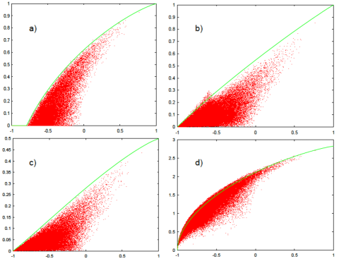
Figure 1: (Color online) Plot of the dependency of a) concurrence, b) quantum discord, c) geometric discord and c) maximum violation of CHSH Bell inequality vs. the minimum of the negative quantities in (4) in units of $\ln 2$, for a sample of $10^{6}$ random states. In all cases, we appreciate a strong correlation. The solid (green) line depicts the case for Werner states. See text for details.

What is depicted in Fig. 1 are several quantum correlation measures versus the minimum of both two quantities appearing in the definition of conditional entropies. From the figure, we can see that the areas with low values of quantum correlations are strongly populated with states that violate the entropic inequalities (negative horizontal axis). Although considerably less, one can find states (very few) not violating any entropic inequality (positive horizontal axis) with high values of quantum correlations, which proves that entropic criteria fail considerably. The functional dependency between violation of entropic inequalities and existence of non-zero quantum correlations must be interpreted as follows: states violating the entropic criteria lie very close to zero or small quantum correlation values. Staying within the negative horizontal axis, as we move to the right, we tend to find less population of states with higher and higher values of quantal correlations. Therefore, the correlation between entropic measures (their violation) and quantum measures should be better understood if we restrict ourselves to the negative horizontal axis.

The numerical survey over all states (a sample of a million mixed states in our case) displays very interesting results when i) the whole set of states is considered, and when ii) states are discriminated according to their degree of mixture $R=1/Tr(\rho^{2})$. We could have used the so-called purity $Tr(\rho^{2})$ instead as a degree of mixture. However, one being the inverse of the other, they provide the same information regarding the degree of mixture $R$ of the state $\rho$. When we consider the probability that the entropic criteria and any other measure providing the same answer, we arrive at these corresponding results:

• entropic inequalities and entanglement: there is a probability of $64.3\%$ that an arbitrary state either violates (fulfills) the entropic inequalities with non-zero (null) entanglement.

• entropic inequalities and the CHSH Bell inequality: there is a probability of $99.4\%$ that an arbitrary state either violates (fulfills) the entropic inequalities with maximal CHSH violation less than –that is, local– (greater than –that is, nonlocal–) two.

In addition, it is seen that both entanglement and nonlocality have a concomitant probability of $64.6\%$ of coincidence.

When we use a particular family of states, the Bell diagonal states, the situation becomes the following:

• entropic inequalities and entanglement: there is a probability of $83.6\%$ that an arbitrary state either violates (fulfills) the entropic inequalities with non-zero (null) entanglement.

• entropic inequalities and the CHSH Bell inequality: there is a probability of $99.4\%$ that an arbitrary state either violates (fulfills) the entropic inequalities with maximal CHSH violation less than –that is, local– (greater than –that is, nonlocal–) two.

Entanglement and nonlocality have a concomitant probability of $84.2\%$ of coincidence. As it can be appreciated, there is a considerable, almost perfect correlation between entropic inequalities and nonlocality, whereas the coincidence is lower when comparing with entanglement.

When states are generated with a given value of $R$, the concomitant probabilities of coincidence display a very surprising behavior. In Fig. 2, the probability of both entropic criterion and entanglement leading to the same answer (lower curve) and the same thing for entropic and nonlocality (upper curve) are depicted, respectively. It is apparent from our calculations that all states with degree of mixture $R$ between 2 and 3 do not violate any entropic inequality, and the same thing happens for nonlocality: all states are local as well, that is, their maximal CHSH Bell quantity is always less than or equal to 2. Thus, both entropic and Bell inequalities provides the same answer in the aforementioned region. Therefore, the probability of coincidence is exactly 1.

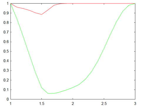
Figure 2: (Color online) Probability of coincidence between concurrence and entropic inequalities (lower curve), and coincidence between CHSH Bell inequalities and entropic inequalities (upper curve) vs. $R$. In the latter case, small discrepancies appear nearby pure states ($R=1$). Every point has been obtained generating $10^{6}$ random states with the same mixture $R$ (see Appendix II). See text for details.

Now we are going to summarize and to prove the previous facts with respect to all states with a given degree of mixture, either given by $R$ or the maximum eigenvalue $\lambda_{m}$ of a state $\rho$, in the following theorems:

Proposition 1: If the participation ratio $R=1/Tr(\rho^{2})$ is given to be $R\in[2,4]$, then the maximum eigenvalue $\lambda_{m}$ of $\rho$ is bounded inside $\lambda_{m}\in[\frac{1}{4},1/\sqrt{2}\approx 0.7)$.

Proof: The condition $R\geq 2$ is equivalent to $\lambda_{1}^{2}+\lambda_{2}^{2}+\lambda_{3}^{2}+\lambda_{4}^{2}\leq 1/2$. Now, the minimum value for $\lambda_{1}$ is clearly 1/4 because no eigenvalue is greater that their arithmetic mean. The maximum is obtained as follows: From the squares of the eigenvalues, it is plain that $\lambda_{1}^{2}<1/2$, or $\lambda_{1}<0.7$. Thus, $\lambda_{1}\in[\frac{1}{4},0.7)$ $\blacksquare$

Proposition 2: If the maximum eigenvalue of a state $\rho$ is given to be $\lambda_{m}\leq 1/2$, then we have $R\in[2,4]$.

Proof: If $\lambda_{1}\leq 1/2$, then the same condition applies to all the rest $\lambda_{i}\leq 1/2$. Therefore, we can define the quantities $\lambda_{i}(1/2-\lambda_{i})$ to be obviously positive. When developing them, we have $\frac{1}{2}\lambda_{i}\geq\lambda_{i}^{2}$. By adding the whole set of inequalities $i=1..4$, we encounter that $\lambda_{1}^{2}+\lambda_{2}^{2}+\lambda_{3}^{2}+\lambda_{4}^{2}\leq 1/2$, which is tantamount as having $R\geq 2$ $\blacksquare$

With these two propositions, we are about to prove one of the major results of the present work for two qubit states.

Theorem 1 ($R$-language) For all mixed states $\rho$ fulfilling $R\in[2,4]$, these two statements are equivalent:

• There is no violation of the entropic inequalities

• No Bell inequality is violated (specifically, the CHSH inequality)

Proof: Let us proof the first statement. The non-violation of entropic inequalities requires $S(\rho_{AB})-S(\rho_{A})\geq 0$ and $S(\rho_{AB})-S(\rho_{B})\geq 0$. Suppose that $\lambda_{1}>\lambda_{2}>\lambda_{3}>\lambda_{4}$ is the set of eigenvalues of an arbitrary state of two qubits. Formally, we have that $-\lambda_{1}\ln\lambda_{1}-\lambda_{2}\ln\lambda_{2}-\lambda_{3}\ln\lambda_{3}-\lambda_{4}\ln\lambda_{4}-(-\alpha\ln\alpha-(1-\alpha)\ln(1-\alpha))\geq 0$, where $\alpha$ and $1-\alpha$ are the eigenvalues of the reduced density matrices ($\alpha\in[0,1]$). The same expression can be written more compactly as

$$\lambda_{1}^{\lambda_{1}}\lambda_{2}^{\lambda_{2}}\lambda_{3}^{\lambda_{3}}\lambda_{4}^{\lambda_{4}}\leq\alpha^{\alpha}(1-\alpha)^{(1-\alpha)}$$ (8)

$\alpha^{\alpha}(1-\alpha)^{(1-\alpha)}$ is a monotonically decreasing function of $\alpha$, ranging from 1 to 1/2 for $\alpha\in[0,1]$. Since, according to Proposition 1, we have that the maximum eigenvalue $\lambda_{1}\leq 0.7$, then all other eigenvalues $\lambda_{i}$ must also be less than 0.7. Plugging the aforementioned values into (8), we have

$$0.7^{0.7}\cdot 0.7^{0.7}\cdot 0.7^{0.7}\cdot 0.7^{0.7}<0.37<\alpha^{\alpha}(1-\alpha)^{(1-\alpha)}<1.$$ (9)

That is, no violation of the entropic inequalities occurs $\blacksquare$

Let us prove the second statement. It will be suitable to have the arbitrary state of two qubits written in the Bloch representation

$$4\rho=\mathcal{I}\otimes\mathcal{I}+\sum_{u=1}^{3}x_{u}\sigma_{u}\otimes\mathcal{I}+\sum_{u=1}^{3}y_{u}\mathcal{I}\otimes\sigma_{i}+\sum_{u,v=1}^{3}T_{uv}\sigma_{u}\otimes\sigma_{v},$$ (10)

with $x_{u}=Tr(\rho(\sigma_{u}\otimes\mathcal{I}))$, $y_{u}=Tr(\rho(\mathcal{I}\otimes\sigma_{u}))$, and $T_{uv}=Tr(\rho(\sigma_{u}\otimes\sigma_{v}))$. These parameters form the correlation matrix (30). Let us multiply the state by itself and take the trace. Then $Tr(\rho^{2})=\frac{1}{4}[1+\sum_{i}x_{i}^{2}+\sum_{i}y_{i}^{2}+\sum_{i,j}T_{ij}^{2}]$, which is equal to $1/R$. $R\geq 2$ implies $1/R\leq 1/2$, which combined with the previous quantities gives us

$$\sum_{i}x_{i}^{2}+\sum_{i}y_{i}^{2}+\sum_{i,j}T_{ij}^{2}\leq 1.$$ (11)

The former fact implies that

$$\sum_{i,j}T_{ij}^{2}\leq 1-(\sum_{i}x_{i}^{2}+\sum_{i}y_{i}^{2}),$$ (12)

which it has to be a positive quantity. From the work developed by Horodecki et al in HoroBell regarding necessary and sufficient conditions for the violation of the CHSH Bell inequality, we have that the quantity $M(\rho)\equiv max_{\bf{c},\bf{c^{\prime}}}\big{(}||T\bf{c}||^{2}+||T\bf{c^{\prime}}||^{2}$, where $T$ is the matrix defined by $T_{ij}$ ($\bf{c,c^{\prime}}$ are suitable unit vectors), has to be less than 1 in order not to violate the CHSH Bell inequality. Since the bound $M(\rho)\leq\sum_{i,j}T_{ij}^{2}$ holds, it is plain from (12) that $M(\rho)\leq 1-(\sum_{i}x_{i}^{2}+\sum_{i}y_{i}^{2})<1$, which finishes the proof $\blacksquare$

As we can appreciate, the previous result is similar to the one relating unentangled states for all $R\geq 3$, although in our case we deal with nonlocality. Thus, if a state is mixed enough, it will not possess any nonlocality from $R=2$ onward, yet it can be entangled. However, if it is is much more mixed, then all entanglement disappears.

If we measure the degree of mixture by the maximum eigenvalue of the state, then we shall have a similar theorem:

Theorem 2 ($\lambda_{m}$-language) For all mixed states $\rho$ fulfilling $lambda_{m}\leq 1/2$, these two statements are equivalent:

• There is no violation of the entropic inequalities

• No Bell inequality is violated (specifically, the CHSH inequality)

Proof: The first sentence can be easily proved in the same fashion that in Theorem 1. Substituting $0.7$ by $0.5$ the bound still holds and that finishes the proof $\blacksquare$

The second sentence is proved in a straightforward manner. Owing to Proposition 2, $\lambda_{m}\leq 1/2$ implies $R\geq 2$, which constitutes the second statement of Theorem 1 $\blacksquare$

We can summarize the situation in the following way:

• For $R\in[1,2)$ nonlocality, violation of entropic inequalities and entanglement coexist

• For $R\in[2,3]$ nonlocality disappears, entropic inequalities are not violated and entanglement is still present

• For $R\in[3,4]$ neither nonlocality, nor violation of entropic inequalities nor entanglement are present

or use the $\lambda_{m}$ approach instead: for any state with $\lambda_{m}\leq 2$ both non violation of entropic inequalities and CHSH Bell inequalities occur. For $\lambda>1/2$, Bell inequalities can be violated (they are in all cases for Bell diagonal states), whereas entanglement is not always present (certainly it is in the Bell diagonal case only). It is worth mentioning that when discriminating the values for the conditional entropies for all states vs. either $R$ or $\lambda_{m}$, there appear several regions that are bounded by certain states, which will be described somewhere else.

Summing up, we have described a positive correlation between usual quantum measures such as discord, entanglement or nonlocality and the violation of entropic inequalities, quantified by the conditional entropy of each subsystem A and B. In addition, in the simplest case of two qubits, the degree of coincidence between entropic and Bell inequalities is surprisingly high, which is surprising taking into account the different nature of the magnitudes being represented. This previous fact allow us to shed new light on the classical nature of entropic inequalities for witnessing entanglement and the concomitant relation with nonlocality, given by the violation of the CHSH Bell inequality.

II.2 Three qubits

In the case of three qubits, no other measure similar to discord exists. Only entanglement and nonlocality, which is given by the maximum violation of the Mermin inequality, described in Appendix II along with the concomitant optimization techniques. The Mermin, Ardehali, Belinskii and Klyshko (MABK) inequalities (for $n=3$, the Mermin one) are not the only existing Bell inequalities for $n$ qubits MABKnew ; Ref1 ; Ref2 , but they constitute a simple generalization of the CHSH one to the multipartite case. Accordingly, it will suffice to use these particular inequalities to illustrate the basic results of the present work, as far as non-locality is concerned.

For three qubits, the entropic inequalities read

$$S(\rho_{ABC})-S(\rho_{A}) \geq 0$$ (13)

$$S(\rho_{ABC})-S(\rho_{B}) \geq 0$$ (14)

$$S(\rho_{ABC})-S(\rho_{C}) \geq 0,$$ (15)

where $S$ is the usual von Neumann entropy $S_{1}$. When developing into the corresponding states and reduced states, we have the corresponding expression for the spectra of eigenvalues

$$\lambda_{1}^{\lambda_{1}}\lambda_{2}^{\lambda_{2}}\lambda_{3}^{\lambda_{3}}\lambda_{4}^{\lambda_{4}}\lambda_{5}^{\lambda_{5}}\lambda_{6}^{\lambda_{6}}\lambda_{7}^{\lambda_{7}}\lambda_{8}^{\lambda_{8}} \leq \alpha^{\alpha}(1-\alpha)^{1-\alpha}$$ (16)

$$\lambda_{1}^{\lambda_{1}}\lambda_{2}^{\lambda_{2}}\lambda_{3}^{\lambda_{3}}\lambda_{4}^{\lambda_{4}}\lambda_{5}^{\lambda_{5}}\lambda_{6}^{\lambda_{6}}\lambda_{7}^{\lambda_{7}}\lambda_{8}^{\lambda_{8}} \leq \beta^{\beta}(1-\beta)^{1-\beta}$$ (17)

$$\lambda_{1}^{\lambda_{1}}\lambda_{2}^{\lambda_{2}}\lambda_{3}^{\lambda_{3}}\lambda_{4}^{\lambda_{4}}\lambda_{5}^{\lambda_{5}}\lambda_{6}^{\lambda_{6}}\lambda_{7}^{\lambda_{7}}\lambda_{8}^{\lambda_{8}} \leq \gamma^{\gamma}(1-\gamma)^{1-\gamma},$$ (18)

where we can assume similar conditions ($n=2$ qubits) for the eigenvalues $\{\lambda_{i}\}$ of the state $\rho_{ABC}$ and those ones $\{\alpha,1-\alpha,\beta,1-\beta,\gamma,1-\gamma\}$ for the reduced density matrices.

Our numerical survey taken on the whole set of mixed states of three qubits shows that for $R\leq 1.5$ all states violate (13). We are going to provide a rough estimate for the boundary as follows. Suppose that we relax the conditions in (16) such that all reduced eigenvalues can be reduced to a single expression. In addition, let us remember that the maximum eigenvalue of $\rho_{ABC}$ is given by $\lambda_{1}$. Then, all other eigenvalues would be less that $\lambda_{1}$, which leads us to the following inequality to fulfill the entropic inequalities:

$$\lambda_{1}^{\lambda_{1}}\lambda_{2}^{\lambda_{2}}\lambda_{3}^{\lambda_{3}}\lambda_{4}^{\lambda_{4}}\lambda_{5}^{\lambda_{5}}\lambda_{6}^{\lambda_{6}}\lambda_{7}^{\lambda_{7}}\lambda_{8}^{\lambda_{8}}<(\lambda_{1}^{\lambda_{1}})^{8}\leq\alpha^{\alpha}(1-\alpha)^{1-\alpha}<1.$$ (19)

Let us find $\lambda_{1}$ such that the inequality is independent of $\alpha$ by setting the equation $(\lambda_{1}^{\lambda_{1}})^{8}=1/2$ (recall that $\alpha^{\alpha}(1-\alpha)^{1-\alpha}$ is bounded between 1/2 and 1). The solutions to the previous transcendental equation are 0.90909 and 0.0229, but only the first one is valid because $\lambda_{1}>1/8$. It can be easily proved that $\lambda_{1}=0.90909$ implies a maximum $R\approx 1.2$. Thus, a rough estimate of the minimum $R$ such that all states do not violate (13) is found, which is a bit smaller than the numerically observed 1.5.

Not much is know about nonlocality and entanglement in more than two parties. However, some important results have been obtained which are relevant. Following the exact treatment of maximum nonlocality in multiqubit states JPhysAnostro2011 , it is found that

$$Mermin^{\max}(R)\propto\sqrt{\frac{8-R}{8R}},$$ (20)

where the constant in (20) is obtained by requiring $Mermin^{\max}$ to be equal to 4 for pure states ($R=1$). One class of states that possess the previous optimal value is $\rho^{diag}=(1-7x,x,x,x,x,x,x,x)$, which is, interestingly enough, the generalized Werner state for three qubits

$$\rho_{W}^{n=3}=\tilde{x}|GHZ\rangle\langle GHZ|+\frac{1-\tilde{x}}{8}I_{8},$$ (21)

where $I_{8}$ is the $8\times 8$ identity matrix, and $\tilde{x}=1-8x$. Notice that this was not the case for the two qubit instance.

This interesting feature enables us to discuss the different ranges for $R$ where to compare nonlocality and presence of genuine tripartite entanglement. On the one hand, from (20) we obtain the nonlocality critical value $R_{1}=32/11\approxeq 2.9$: no three qubit states possess any nonlocality for participation ratios $R\geq R_{1}$. On the other hand, the special nature of generalized Werner states allow us to compute the separability threshold between entanglement and separability WernerThreshold . From Ref. WernerThreshold , the contribution $\tilde{x}$ in (21) is such that $x\leq 1/5$ involves absence of entanglement. Translated into $R$-language, it implies a second critical value $R_{2}=25/4=6.25$: no three qubit states possess entanglement for participation ratios $R\geq R_{2}$.

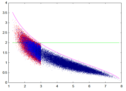
Figure 3: (Color online) Plot of the maximum violation of the Mermin inequality for $n=3$ qubits vs. $R$. The region between $R=1$ and $R=3$ has been enhanced so that it can be appreciate that all states beyond $R_{1}=32/11\approxeq 2.9$ are local. See text for details.

Therefore, the range of $R$-values splits into three regions: i) between 1 (pure states) and $R_{1}$, maximum amounts of nonlocality imply the presence of entanglement; ii) between $R_{1}$ and $R_{2}$ we have no violation of the Mermin inequality, yet there exists entanglement; finally, iii) region between $R_{2}$ and $R=8$ (maximally mixed state) displays absence of both magnitudes. We have to mention that our numerical survey for all state agrees with the nonlocality boundary described previously. In Fig. 3 a sample of states is shown where the maximum violation of the Mermin inequality is depicted vs. the degree of mixture $R$. The solid line corresponds to (20). Notice that the Mermin inequality is violated for values greater than 2.

When gathering the results obtained from the entropic inequalities, the whole situation looks quite interesting, as depicted in Fig. 4. The boundaries for entropic inequalities are not strictly defined analytically, whereas the nonlocality region is exact. The region with zero entanglement is estimated via the only known result for three qubits, that is, the Werner state. Therefore it is likely that $R_{2}$ could be a bit bigger than the actual (unknown) value. In any case, we can appreciate the great extraordinary coincidence between the non-violation of the classical entropic inequalities and the non-violation of the Mermin Bell inequality, in addition to a hierarchy of criteria entropic-nonlocality-entanglement as the degree of mixture increases. In other words, if classicality is described by fulfilling the entropic inequalities and locality by not violating any Local Variable Model bound, we have found here that both quantities coincide to a very great extend, although being very different in nature. Only for states quite close to pure states most quantum measures coincide.

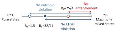
Figure 4: (Color online) Plot of the situation regarding locality, reality and entanglement ranges when states of three qubits are discriminated according to their degree of mixture $R$. See text for details.

II.3 Four qubits

When discussing higher number multiqubit states, our knowledge about quantum correlations is very limited. Alas, no real measure for entanglement exists and only violation of maximum Bell inequalities can be performed. Furthermore, the application of the entropic inequalities becomes quantitatively more involved, since a set of $2^{n-1}-1$ inequalities must be studied, which correspond to all bipartite divisions of the state $\rho$ into subsystems.

However, our numerical exploration shows in Fig. 5 that all states are likely to fulfill the concomitant entropic inequalities for $R\in[3,16]$, whereas all states seem to fulfill the locality requirements for the corresponding MABK Bell inequality for $R\in[4,16]$. What we see again is a great coincidence between locality and classicality, the same hierarchy as in previous cases and a dilatation of the regions where they both appear. It seems plausible to think that the tendency for higher $n$ systems is that the region where locality and classicality coincide extends, which provides a useful tool for ascertaining nonlocality (and entanglement) through the use of a simple, classical entropic criteria. And, indeed, this is the case.

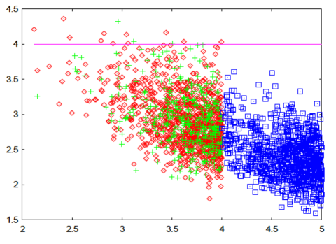
Figure 5: (Color online) Plot of the maximum violation of the MABK inequality for $n=4$ qubits vs. $R$. It is apparent that beyond $R=4$ no MABK violation occurs. See text for details.

Although the study of arbitrary quantum correlations in higher dimensions becomes really involved, if we take the easy case of generalized Werner states, the maximum violation of the concomitant MABK Bell inequalities (let us consider $n$ the number of qubits to be an even number, the well-known “Ardehali” MABK Bell inequality) can be obtained. It is $2^{\frac{n+1}{2}}\cdot p$, linear with the weight $p\in[0,1]$, corresponding to $|GHZ\rangle_{n}$. Now, when finding the value for the critical value $p_{c}$ such that below this value no violation occurs (we suppose an idealized case with efficiency of all detectors $\eta=1$), we find that it is exactly the inverse of the amount by which quantum mechanics exceeds LVM predictions, which is an exponentially large factor. Therefore, when considering the number of qubits $n$ large enough, we encounter that $p_{c}\rightarrow 0$ . That is, as we increase the number of qubits, generalized Werner states tend to have no violation of the concomitant MABK Bell inequalities or, in other words, the range where nonlocality can be found is infinitesimally closer to pure states ($R=1$). This previous fact does not imply that a nonlocal state could be found for $R>1$, but certainly the general trend will be that nonlocality will be found only very close to pure states. And if that is the case, we shall expect both classical entropic inequalities and MABK Bell inequalities to provide the same answer for a given state $\rho$. Summing up, when we are dealing with mixed states, as the number of qubits increases, locality and classicality become identical.

III Conclusions

We have explored the whole set of states for different multiqubit systems and have discovered an intimate relationship between locality and classicality. The concomitant results shed new light on the strange connection existing between them when the whole set of states is considered and, in particular, when they are compared with states with the same amount of mixedness. The overall overlap of regions where we have states $\rho$ with no entropic violation - no nonlocality - no entanglement as we increase their mixture is quite surprising, although a bit expected for the increasing tendency of states towards maximally mixed ones suggests that no quantum correlations survive. This tendency is checked to extend as we increase the number of parties and, eventually, for higher enough subsystems, they become almost identical. Thus, the non violation of entropic inequalities constitute a close first approximation to detecting quantum correlations and, therefore, reducing the usual number of computations either for Bell correlations or quantum tomography for entanglement-like measurements.

APPENDIX I: Definition and calculation of quantal measures

For the quantum discord QD, a minimization takes place for two parameters only, whereas non-locality $MABK_{N}^{\max}$ requires an exploration among their corresponding unit vectors defining the observers’ settings. In any case, we have performed a two-fold search employing i) an amoeba optimization procedure, where the optimal value is obtained at the risk of falling into a local minimum and ii) the well known simulated annealing approach kirkpatrick83 . The advantage of this computational ’duplicity’ is that we can be confident regarding the final results reached. Indeed, the second recipe contains a mechanism that allows for local searches that eventually can escape local optima.

III.1 Quantum discord

Quantum discord olli constitutes a quantitative measure of the “non-classicality” of bipartite correlations as given by the discrepancy between the quantum counterparts of two classically equivalent expressions for the mutual information. More precisely, quantum discord is defined as the difference between two ways of expressing (quantum mechanically) such an important entropic quantifier. If $S$ stands for the von Neumann entropy, for a bipartite state $A-B$ of density matrix $\rho$ and reduced (“marginals”) ones $\rho_{A}$-$\rho_{B}$, the quantum mutual information (QMI) $M_{q}$ reads olli

$$M_{q}(\rho)=S(\rho_{A})+S(\rho_{B})-S(\rho),$$ (22)

which is to be compared to its associated classical notion $M_{class}(\rho)$, that is expressed using conditional entropies. If a complete projective measurement $\Pi_{j}^{B}$ is performed on B and (i) $p_{i}$ stands for $Tr_{AB}\,\Pi_{i}^{B}\,\rho$ and (ii) $\rho_{A||\Pi_{i}^{B}}$ for $[\Pi_{i}^{B}\,\rho\,\Pi_{i}^{B}/p_{i}]$, then our conditional entropy becomes

$$S(A|\,\{\Pi_{j}^{B}\})=\sum_{i}\,p_{i}\,S(\rho_{A||\Pi_{i}^{B}}),$$ (23)

so that $M_{class}(\rho)$ adopts the appearance

$$M_{class}(\rho)_{\{\Pi_{j}^{B}\}}=S(\rho_{A})-S(A|\,\{\Pi_{j}^{B}\}).$$ (24)

Now, if we minimize over all possible $\Pi_{j}^{B}$ the difference $M_{q}(\rho)-M_{class}(\rho)_{\{\Pi_{j}^{B}\}}$ we obtain the quantum discord $\Delta$, that quantifies non-classical correlations in a quantum system, including those not captured by entanglement. The most general parameterization of the corresponding local measurements that can be implemented on one qubit (let us call it B) is of the form $\{\Pi_{B}^{0^{\prime}}=I_{A}\otimes|0^{\prime}\rangle\langle 0^{\prime}|,\Pi_{B}^{1^{\prime}}=I_{A}\otimes|1^{\prime}\rangle\langle 1^{\prime}|\}$. More specifically we have

$$|0^{\prime}\rangle \leftarrow \cos\alpha^{\prime}|0\rangle+e^{i\beta^{\prime}}\sin\alpha^{\prime}|1\rangle$$ (25)

$$|1^{\prime}\rangle \leftarrow e^{-i\beta^{\prime}}\sin\alpha^{\prime}|0\rangle-\cos\alpha^{\prime}|1\rangle,$$ (26)

which is obviously a unitary transformation –rotation in the Bloch sphere defined by angles $(\alpha^{\prime},\beta^{\prime})$– for the B basis $\{|0\rangle,|1\rangle\}$ in the range $\alpha^{\prime}\in[0,\pi]$ and $\beta^{\prime}\in[0,2\pi)$. The previous computation of the QD has to be carried out numerically, unless the two qubit states belong to the class of the so called X-states, where QD is analytic Xstates . One notes then that only states with zero $\Delta$ may exhibit strictly classical correlations.

III.2 Geometric quantum discord

Despite increasing evidences for relevance of the quantum discord (Qd) in describing non-classical resources in information processing tasks, there was until quite recently no straightforward criterion to verify the presence of discord in a given quantum state. Since its evaluation involves an optimization procedure and analytical results are known only in a few cases, such criteria become clearly desirable. Recently, Datta advanced a condition for nullity of quantum discord datta , and progress was also achieved in geom by introducing an interesting geometric measure of quantum discord (GQD). Let $\chi$ be a generic $\Delta=0-$state. The GQD measure is then given by

$$D(\rho)={\rm Min}_{\chi}[||\rho-\chi||^{2}],$$ (27)

where the minimum is over the set of zero-discord states $\chi$. We deal then with the square of Hilbert-Schmidt norm of Hermitian operators, $||\rho-\chi||^{2}=Tr[(\rho-\chi)^{2}]$ . Dakic et al. show how to evaluate this quantity for an arbitrary two-qubit state geom ; luo . Moreover, they demonstrate the their geometric distance contains all relevant information associated to the notion of quantum discord. This was a remarkable feat given that, despite robust evidence for the pertinence of the Qd-notion, its evaluation involves optimization procedures, with analytic results being known only in a few cases.

Now, given the general form of an arbitrary two-qubits’ state in the Bloch representation

$$4\rho=\mathcal{I}\otimes\mathcal{I}+\sum_{u=1}^{3}x_{u}\sigma_{u}\otimes\mathcal{I}+\sum_{u=1}^{3}y_{u}\mathcal{I}\otimes\sigma_{i}+$$ (28)

$$+\sum_{u,v=1}^{3}T_{uv}\sigma_{u}\otimes\sigma_{v},$$ (29)

with $x_{u}=Tr(\rho(\sigma_{u}\otimes\mathcal{I}))$, $y_{u}=Tr(\rho(\mathcal{I}\otimes\sigma_{u}))$, and $T_{uv}=Tr(\rho(\sigma_{u}\otimes\sigma_{v}))$, it is found in Ref. geom that a necessary and sufficient criterion for witnessing non-zero quantum discord is given by the rank of the correlation matrix

$$\frac{1}{4}\left(\begin{array}[]{cccc}1&y_{1}&y_{2}&y_{3}\\ x_{1}&T_{11}&T_{12}&T_{13}\\ x_{2}&T_{21}&T_{22}&T_{23}\\ x_{3}&T_{31}&T_{32}&T_{33}\end{array}\right),$$ (30)

that is, a state $\rho$ of the form (28) exhibits finite quantum discord iff the matrix (30) has a rank greater that two. It is seen that the geometric measure (27) is of the final form geom

$$D(\rho)=\frac{1}{4}\bigg{(}||{\bf x}||^{2}+||T||^{2}-\lambda_{\max}\bigg{)}=$$ (31)

$$=\frac{1}{R}-\frac{1}{4}-\frac{1}{4}\bigg{(}||{\bf y}||^{2}+\lambda_{\max}\bigg{)},$$ (32)

where $||{\bf x}||^{2}=\sum_{u}x_{u}^{2}$, and $\lambda_{\max}$ is the maximum eigenvalue of the matrix $(x_{1},x_{2},x_{3})^{t}(x_{1},x_{2},x_{3})+TT^{t}$. Here the superscript $t$ denotes either vector or matrix transposition. The second expression emphasizes the natural dependence of $D$ on the participation ratio $R=1/Tr(\rho^{2})$. Notice that this measure is intimately connected with the quantities appearing in (30).

III.3 Violation of MABK inequalities

Most of our knowledge on Bell inequalities and their quantum mechanical violation is based on the CHSH inequality CHSH . With two dichotomic observables per party, it is the simplest Collins (up to local symmetries) nontrivial Bell inequality for the bipartite case with binary inputs and outcomes. Let $A_{1}$ and $A_{2}$ be two possible measurements on A side whose outcomes are $a_{j}\in\{-1,+1\}$, and similarly for the B side. Mathematically, it can be shown that, following LVM, $|{\cal B}_{CHSH}^{LVM}(\lambda)|=|a_{1}b_{1}+a_{1}b_{2}+a_{2}b_{1}-a_{2}b_{2}|\leq 2$. Since $a_{1}$($b_{1}$) and $a_{2}$($b_{2}$) cannot be measured simultaneously, instead one estimates after randomly chosen measurements the average value ${\cal B}_{CHSH}^{LVM}\equiv\sum_{\lambda}{\cal B}_{CHSH}^{LVM}(\lambda)\mu(\lambda)=E(A_{1},B_{1})+E(A_{1},B_{2})+E(A_{2},B_{1})-E(A_{2},B_{2})$, where $E(\cdot)$ represents the expectation value. Therefore the CHSH inequality reduces to

$$|{\cal B}_{CHSH}^{LVM}|\leq 2.$$ (33)

Quantum mechanically, since we are dealing with qubits, these observables reduce to ${\bf A_{j}}({\bf B_{j}})={\bf a_{j}}({\bf b_{j}})\cdot{\bf\sigma}$, where ${\bf a_{j}}({\bf b_{j}})$ are unit vectors in $\mathbb{R}^{3}$ and ${\bf\sigma}=(\sigma_{x},\sigma_{y},\sigma_{z})$ are the usual Pauli matrices. Therefore the quantal prediction for (33) reduces to the expectation value of the operator ${\cal B}_{CHSH}$

$${\bf A_{1}}\otimes{\bf B_{1}}+{\bf A_{1}}\otimes{\bf B_{2}}+{\bf A_{2}}\otimes{\bf B_{1}}-{\bf A_{2}}\otimes{\bf B_{2}}.$$ (34)

Tsirelson showed Tsirelson that CHSH inequality (33) is maximally violated by a multiplicative factor $\sqrt{2}$ (Tsirelson’s bound) on the basis of quantum mechanics. In fact, it is true that $|Tr(\rho_{AB}{\cal B}_{CHSH})|\leq 2\sqrt{2}$ for all observables ${\bf A_{1}}$, ${\bf A_{2}}$, ${\bf B_{1}}$, ${\bf B_{2}}$, and all states $\rho_{AB}$. Increasing the size of Hilbert spaces on either A and B sides would not give any advantage in the violation of the CHSH inequalities. In general, it is not known how to calculate the best such bound for an arbitrary Bell inequality, although several techniques have been developed Toner .

A good witness of useful correlations is, in many cases, the violation of a Bell inequality by a quantum state. Therefore we shall consider the optimization of the violation of the CHSH inequality over the observer’s settings as a definitive measure for both signaling and quantifying nonlocality in two qubit systems.

We are going to determine which is the maximum expectation value of the CHSH operator (34) that a two qubit mixed state $\rho$ with some degree of mixedness, in this case given by the so called participation ratio $R=1/Tr(\rho^{2})$, may have. Notice that no assumption is needed regarding the state being diagonal or not in the Bell basis. In order to solve the concomitant variational problem (and bearing in mind that $B_{CHSH}=Tr(\rho{\cal B}_{CHSH})$), let us first find the state that extremizes Tr($\rho^{2}$) under the constraints associated with a given value of $B_{CHSH}$, and the normalization of $\rho$. This variational problem can be cast as

$$\delta\big{[}Tr(\rho^{2})+\beta Tr(\rho{\cal B}_{CHSH})-\alpha Tr(\rho)\big{]}=0,$$ (35)

where $\alpha$ and $\beta$ are appropriate Lagrange multipliers. After some algebra, we arrive at the result

$$B_{CHSH}^{\max}=\sqrt{Tr[{\cal B}_{CHSH}^{2}]}\cdot\sqrt{\frac{4-R}{4R}}=4\cdot\sqrt{\frac{4-R}{4R}}.$$ (36)

This result is valid for the range $R\in[2,4]$. In the region $R\in[1,2]$ we obtain

$$B_{CHSH}^{\max}=\sqrt{\frac{8}{R}}.$$ (37)

We shall explore nonlocality in the three qubit case through the violation of the Mermin inequality Mermin . This inequality was conceived originally in order to detect genuine three-party quantum correlations impossible to reproduce via LVMs. The Mermin inequality reads as $Tr(\rho{\cal B}_{Mermin})\leq 2$, where ${\cal B}_{Mermin}$ is the Mermin operator

$${\cal B}_{Mermin}=B_{a_{1}a_{2}a_{3}}-B_{a_{1}b_{2}b_{3}}-B_{b_{1}a_{2}b_{3}}-B_{b_{1}b_{2}a_{3}},$$ (38)

with $B_{uvw}\equiv{\bf u}\cdot{\bf\sigma}\otimes{\bf v}\cdot{\bf\sigma}\otimes{\bf w}\cdot{\bf\sigma}$ with ${\bf\sigma}=(\sigma_{x},\sigma_{y},\sigma_{z})$ being the usual Pauli matrices, and ${\bf a_{j}}$ and ${\bf b_{j}}$ unit vectors in $\mathbb{R}^{3}$. Notice that the Mermin inequality is maximally violated by Greenberger-Horne-Zeilinger (GHZ) states. As in the bipartite case, we shall define the following quantity

$$Mermin^{\max}\equiv\max_{\bf{a_{j}},\bf{b_{j}}}\,\,Tr(\rho{\cal B}_{Mermin})$$ (39)

as a measure for the nonlocality of the state $\rho$. While in the bipartite the CHSH inequality was the strongest possible one, this is not the case for three qubits. The Mermin inequality is not the only existing Bell inequality for three qubits, but it constitutes a simple generalization of the CHSH one to the tripartite case. Therefore, it will suffice to use this particular inequality to illustrate the basic results of the present work.

The first Bell inequality for four qubits was derived by Mermin, Ardehali, Belinskii and Klyshko MABK . It constitutes of four parties with two dichotomic outcomes each, being maximum for the generalized GHZ state $(|0000\rangle+|1111\rangle)/\sqrt{2}$. The Mermin-Ardehali-Belinskii-Klyshko (MABK) inequality reads as $Tr(\rho{\cal B}_{MABK})\leq 4$, where ${\cal B}_{MABK}$ is the MABK operator

$$\begin{split}B_{1111}&-B_{1112}-B_{1121}-B_{1211}-B_{2111}-B_{1122}-B_{1212}\\ &-B_{2112}-B_{1221}-B_{2121}-B_{2211}+B_{2222}+B_{2221}\\ &+B_{2212}+B_{2122}+B_{1222},\end{split}$$ (40)

with $B_{uvwx}\equiv{\bf u}\cdot{\bf\sigma}\otimes{\bf v}\cdot{\bf\sigma}\otimes{\bf w}\cdot{\bf\sigma}\otimes{\bf x}\cdot{\bf\sigma}$ with ${\bf\sigma}=(\sigma_{x},\sigma_{y},\sigma_{z})$ being the usual Pauli matrices. As in previous instances, we shall define the following quantity

$$MABK^{\max}\equiv\max_{\bf{a_{j}},\bf{b_{j}}}\,\,Tr(\rho{\cal B}_{MABK})$$ (41)

as a measure for the nonlocality content for a given state $\rho$ of four qubits. ${\bf a_{j}}$ and ${\bf b_{j}}$ are unit vectors in $\mathbb{R}^{3}$. MABK inequalities are such that they constitute extensions of previous inequalities with the requirement that generalized GHZ states must maximally violate them. New inequalities for four qubits have appeared recently (see Ref. MABKnew ) that possess some other states required for optimal violation. In the present study we limit our interest to the MABK inequality, although new ones could be incorporated in order to offer a broader perspective. However, with respect to entanglement, little is know for the quadripartite case, and thus little comparison can be done.

The optimization is taken over the two observers’ settings $\{{\bf a_{j}},{\bf b_{j}}\}$, which are real unit vectors in $\mathbb{R}^{3}$. We choose them to be of the form $(\sin\theta_{k}\cos\phi_{k},\sin\theta_{k}\sin\phi_{k},\cos\theta_{k})$. With this parameterization, the problem consists in finding the supremum of $Tr(\rho{\cal B}_{CHSH})$ over the $\{k=1\dotsm 8\}$ angles of $\{{\bf a_{1}},{\bf b_{1}},{\bf a_{2}},{\bf b_{2}}\}$ that appear in (34).

Optimization of $Mermin^{\max}$ (39) (for states diagonal in the Mermin base of maximally correlated states of three qubits $\rho_{Mermin}^{(diag)}$) is carried out in the same fashion as in the previous bipartite case. Once the observers’ settings $\{{\bf a_{j}},{\bf b_{j}}\}$, which are real unit vectors in $\mathbb{R}^{3}$, are parameterized in spherical coordinates $(\sin\theta_{k}\cos\phi_{k},\sin\theta_{k}\sin\phi_{k},\cos\theta_{k})$, the problem consists in finding the supremum of (39) over the set of $\{k=1\dotsm 12\}$ possible angles for $\{{\bf a_{1}},{\bf b_{1}},{\bf a_{2}},{\bf b_{2}},{\bf a_{3}},{\bf b_{3}}\}$ in (38).

Now, in the case of multiqubit systems, one must instead use a generalization of the CHSH inequality to N qubits. This is done in natural fashion by considering an extension of the CHSH or Mermim inequality to the multipartite case. The first Bell inequality (BI) for four qubits was derived by Mermin, Ardehali, Belinskii, and Klyshko MABK . One deals with four parties with two dichotomic outcomes each, the BI being maximum for the generalized GHZ state $(|0000\rangle+|1111\rangle)/\sqrt{2}$. The Mermin-Ardehali-Belinskii-Klyshko (MABK) inequalities are of such nature that they constitute extensions of older inequalities, with the requirement that generalized GHZ states must maximally violate them. To concoct an extension to the multipartite case, we shall introduce a recursive relation that will allow for more parties. This is easily done by considering the operator

$$B_{N+1}\propto[(B_{1}+B_{1}^{\prime})\otimes B_{N}+(B_{1}-B_{1}^{\prime})\otimes B_{N}^{\prime}],$$ (42)

with $B_{N}$ being the Bell operator for N parties and $B_{1}={\bf v}\cdot{\bf\sigma}$, with ${\bf\sigma}=(\sigma_{x},\sigma_{y},\sigma_{z})$ and ${\bf v}$ a real unit vector. The prime on the operator denotes the same expression but with all vectors exchanged. The concomitant maximum value

$$MABK_{N}^{\max}\equiv\max_{\bf{a_{j}},\bf{b_{j}}}\,\,Tr(\rho{B_{N}})$$ (43)

will serve as a measure for the non-locality content of a given state $\rho$ of N qubits if ${\bf a_{j}}$ and ${\bf b_{j}}$ are unit vectors in $\mathbb{R}^{3}$. The non-locality measure (43) will be maximized by generalized GHZ states, $2^{\frac{N+1}{2}}$ being the corresponding maximum value.

APPENDIX II. Generation of two-qubits states with a fixed value of the participation ratio $R$

The two-qubits case ($N=2\times 2$) is the simplest quantum mechanical system that exhibits the feature of quantum entanglement. One given aspect is that as we increase the degree of mixture, as measured by the so called participation ratio $R=1/$Tr[$\rho^{2}$], the entanglement diminishes (on average). As a matter of fact, if the state is mixed enough, that state will have no entanglement at all. This is fully consistent with the fact that there exists a special class of mixed states which have maximum entanglement for a given $R$ MJWK01 (the maximum entangled mixed states MEMS). These states have been reported to be achieved in the laboratory MEMSexp using pairs of entangled photons. Thus for practical or purely theoretical purposes, it may happen to be relevant to generate mixed states of two-qubits with a given participation ratio $R$.

Here we describe a numerical recipe to randomly generate two-qubit states, according to a definite measure and with a given, fixed value of $R$. Suppose that the states $\rho$ are generated according to the product measure $\nu=\mu\times{\cal L}_{N-1}$, where $\mu$ is the Haar measure on the group of unitary matrices ${\cal U}(N)$ and the standard normalized Lebesgue measure ${\cal L}_{N-1}$ on ${\cal R}^{N-1}$ provides a reasonable computation of the simplex of eigenvalues of $\rho$. In this case, the numerical procedure we are about to explain owes its efficiency to the following geometrical picture which is valid only if the states are supposed to be distributed according to measure $\nu$). We shall identify the simplex $\Delta$ with a regular tetrahedron of side length 1, in ${\cal R}^{3}$, centered at the origin. Let ${\bf r}_{i}$ stand for the vector positions of the tetrahedron’s vertices. The tetrahedron is oriented in such a way that the vector ${\bf r}_{4}$ points towards the positive $z$-axis and the vector ${\bf r_{2}}$ is contained in the $(x,z)$-semiplane corresponding to positive $x$-values. The positions of the tetrahedron’s vertices correspond to the vectors

$$\bf{r_{1}} = (-\frac{1}{2\sqrt{3}},-\frac{1}{2},-\frac{1}{4}\sqrt{\frac{2}{3}})$$

$$\bf{r_{2}} = (\frac{1}{\sqrt{3}},0,-\frac{1}{4}\sqrt{\frac{2}{3}})$$

$$\bf{r_{3}} = (-\frac{1}{2\sqrt{3}},\frac{1}{2},-\frac{1}{4}\sqrt{\frac{2}{3}})$$

$$\bf{r_{4}} = (0,0,\frac{3}{4}\sqrt{\frac{2}{3}}).$$ (44)

The mapping connecting the points of the simplex $\Delta$ (with coordinates $(\lambda_{1},\ldots,\lambda_{4})$) with the points $\bf r$ within tetrahedron is given by the equations

$$\lambda_{i}\, = \,2({\bf r}\cdot{\bf r}_{i})\,+\,\frac{1}{4}\,\,\,\,i=1,\dots,4,$$ (45)

$${\bf r}\, = \,\sum_{i=1}^{4}\lambda_{i}{\bf r}_{i}$$ (46)

The degree of mixture is characterized by the quantity $R^{-1}\equiv Tr(\rho^{2})=\sum_{i}\lambda_{i}^{2}$. This quantity is related to the distance $r=\mid{\bf r}\mid$ to the centre of the tetrahedron $T_{\Delta}$ by

$$r^{2}\,=\,-\frac{1}{8}\,+\,\frac{1}{2}\sum_{i=1}^{4}\lambda_{i}^{2}.$$ (47)

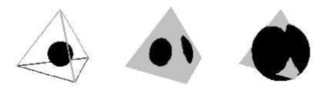
Figure 6: (Color online) Geometric picture of the simplex of eigenvalues (tetrahedron) and a sphere whose radius is related to the degree of mixture $R$. Different growing situations correspond to different regions with definite $R$. See text for details.

Thus, the states with a given degree of mixture lie on the surface of a sphere $\Sigma_{r}$ of radius $r$ concentric with the tetrahedron $T_{\Delta}$. To choose a given $R$ is tantamount to define a given radius of the sphere. There exist three different possible regions (see Fig.6):

• region I: $r\in[0,h_{1}]$ ($R\in[4,3]$), where $h_{1}\equiv h_{c}={1\over 4}\sqrt{2\over{3}}$ is the radius of a sphere tangent to the faces of the tetrahedron $T_{\Delta}$. In this case the sphere $\Sigma_{r}$ lies completely within the tetrahedron $T_{\Delta}$. Therefore we only need to generate at random points over its surface. The Cartesian coordinates for the sphere are given by

  $$x_{1} = r\,\sin\theta\,\cos\phi$$

  $$x_{2} = r\,\sin\theta\,\sin\phi$$

  $$x_{3} = r\,\cos\theta,$$ (48)

  Denoting rand_u() a random number uniformly distributed between 0 an 1, the random numbers $\phi=2\pi$rand_u() and $\theta=\arccos(2$rand_u()$-1)$ (its probability distribution being $P(\theta)=\frac{1}{2}\sin(\theta)$) define an arbitrary state $\rho$ on the surface inside $T_{\Delta}$. The angle $\theta$ is defined between the center of the tetrahedron (the origin) and the vector ${\bf r_{4}}$, and any point aligned with the origin. Substitution of ${\bf r}=(x_{1},x_{2},x_{3})$ in (45) provides us with the eigenvalues $\{\lambda_{i}\}$ of $\rho$, with the desired $R$ as prescribed by the relationship (47). With the subsequent application of the unitary matrices $U$ we obtain a random state $\rho=UD(\Delta)U^{{\dagger}}$ distributed according to the usual measure $\nu=\mu\times{\cal L}_{N-1}$.

• region II: $r\in[h_{1},h_{2}]$ ($R\in[3,2]$), where $h_{2}\equiv\sqrt{h^{2}_{c}+(\frac{D}{2})^{2}}={\sqrt{2}\over 4}$ denotes the radius of a sphere which is tangent to the sides of the tetrahedron $T_{\Delta}$. Contrary to the previous case, part of the surface of the sphere lies outside the tetrahedron. This fact means that we are able to still generate the states $\rho$ as before, provided we reject those ones with negative weights $\lambda_{i}$.

• region III: $r\in[h_{2},h_{3}]$ ($R\in[2,1]$), where $h_{3}\equiv\sqrt{h^{2}_{c}+D^{2}}={\sqrt{6}\over 4}$ is the radius of a sphere passing through the vertices of $T_{\Delta}$. The generation of states is a bit more involved in this case. Again $\phi=2\pi$rand_u(), but the available angles $\theta$ now range from $\theta_{c}(r)$ to $\pi$. It can be shown that $w\equiv\cos(\theta_{c})$ results from solving the equation $3r^{2}w^{2}-\sqrt{\frac{3}{2}}rw+\frac{3}{8}-2r^{2}=0$. Thus, $\theta(r)=\arccos(w(r))$, with $w(r)=\cos\theta_{c}(r)+(1-\cos\theta_{c}(r))$rand_u(). Some states may be unacceptable ($\lambda_{i}<0$) still, but the vast majority are accepted.

Combining these three previous regions, we are able to generate arbitrary mixed states $\rho$ endowed with a given participation ratio $R$.

References

- (1) Hoi-Kwong Lo, S. Popescu and T. Spiller (Editors), Introduction to Quantum Computation and Information (World Scientific, River-Edge, 1998).
- (2) A. Galindo and M. A. Martín-Delgado, Rev. Mod. Phys. 74, 347 (2002).
- (3) M. A. Nielsen and I. L. Chuang, Quantum Computation and Quantum Information (Cambridge University Press, Cambridge, 2000).
- (4) C. P. Williams and S.H. Clearwater, Explorations in Quantum Computing (Springer, New York, 1997).
- (5) C. P. Williams (Editor), Quantum Computing and Quantum Communications (Springer, Berlin, 1998).
- (6) A. Ekert, Phys. Rev. Lett. 67, 661 (1991).
- (7) C.H. Bennett, G. Brassard, C. Crepeau, R. Jozsa, A. Peres and W. K. Wootters, Phys. Rev. Lett. 70, 1895 (1993).
- (8) C. H. Bennett and S. J. Wiesner, Phys. Rev. Lett. 69, 2881 (1993).
- (9) A. Ekert and R. Jozsa, Rev. Mod. Phys. 68, 773 (1996).
- (10) G. P. Berman, G. D. Doolen, R. Mainieri, and V. I. Tsifrinovich, Introduction to Quantum Computers (World Scientific, Sinagapore, 1998).
- (11) B. M. Terhal, Theor. Comp. Sci. 287, 313 (2002).
- (12) R. F. Werner, Phys. Rev. A 40, 4277 (1989).
- (13) A. Peres, Quantum Theory: Concepts and Methods (Kluwer, Dordrecht, 1993).
- (14) M. A. Nielsen and J. Kempe, Phys. Rev. Lett. 86, 5184 (2001).
- (15) M. Horodecki and P. Horodecki, Phys. Rev. A 59, 4206 (1999)
- (16) K. G. H. Vollbrecht and M. M. Wolf, J. Math. Phys. 43, 4299 (2002).
- (17) R. Horodecki, P. Horodecki, M. Horodecki, Phys. Lett. A 210, 377 (1996).
- (18) R. Horodecki, M. Horodecki, Phys. Rev. A 54, 1838 (1996).
- (19) N. Cerf, C. Adami Phys. Rev. Lett. 79, 5194 (1997).
- (20) A. Vidiella-Barranco, Phys. Lett. A 260, 335 (1999).
- (21) C. Tsallis, S. Lloyd, M. Baranger, Phys. Rev. A 63, 042104 (2001).
- (22) C. Tsallis, P.W. Lamberti, D. Prato, Physica A 295, 158 (2001).
- (23) S. Abe, Phys. Rev. A 65, 052323 (2002).
- (24) H. Ollivier and W. H. Zurek, Phys. Rev. Lett. 88, 017901 (2001).
- (25) B. Dakic, V. Vedral and C. Brukner, Phys. Rev. Lett. 105, 190502 (2010).
- (26) A. Ferraro, L. Aolita, D. Cavalcanti, F. M. Cucchietti and A. Acín, Phys. Rev. A 81, 052318 (2010)
- (27) Datta S 2008 Phys. Rev. Lett. 100 050502
- (28) S. Lu and S. Fu, Phys. Rev. A 82, 034302 (2010).
- (29) C. Brukner , M. Zukowski and A. Zeilinger, Phys. Rev. Lett. 89, 197901 (2002).
- (30) J. Barrett J, L. Hardy and A. Kent, Phys. Rev. Lett. 95, 010503 (2005); A. Acín, N. Gisin and Ll. Masanes, Phys. Rev. Lett. 97, 120405 (2006); A. Acín et al. Phys. Rev. Lett. 98, 230501 (2007).
- (31) Karol Bartkiewicz, Bohdan Horst, Karel Lemr, and Adam Miranowicz, Phys. Rev. A 88, 052105 (2013).
- (32) J. F. Clauser, M. A. Horne, A. Shimony, and R. A. Holt, Phys. Rev. Lett. 23, 880 (1969).
- (33) D. Collins and N. Gisin, J. Phys. A: Math. Gen. 37, 1775 (2004).
- (34) R. Horodecki et al., Phys. Lett. A 200, 340 (1995).
- (35) V. Scarani, A. Acín, E. Schenck, and M. Aspelmeyer, Phys. Rev. A 71, 042325 (2005).
- (36) R. F. Werner and M. M. Wolf, Phys. Rev. A 64, 032112 (2001).
- (37) M. Zukowski and C. Brukner, Phys. Rev. Lett. 88, 210401 (2002).
- (38) J. Batle and M. Casas, Phys. Rev. A 82, 062101 (2010); J. Batle and M. Casas, J. Phys. A: Math. Theor. 44, 445304 (2011).
- (39) A. O. Pittenger and M. H. Rubin, Phys. Rev. A 62, 032313 (2006).
- (40) S. Kirkpatrick, C. D. Gelatt Jr., M. P. Vecchi, Science 220, 671 (1983).
- (41) M. Ali, A. R. P. Rau, G. Alber, Phys. Rev. A 81, 042105 (2010).
- (42) S. Datta, arXiv [quant-ph] 1003.5256.
- (43) D. Collins and N. Gisin, J. Phys. A 37, 1775 (2004).
- (44) B. S. Tsirelson, Lett. Math. Phys. 4, 93 (1980); B. S. Tsirelson, J. Soviet Math. 36, 557 (1987); B. S. Tsirelson, Hadronic Journal Supplement 8, 329 (1993).
- (45) B. Toner, Proc. R. Soc. A 465, 59 (2009)
- (46) N. D. Mermin, Phys. Rev. Lett. 65, 1838 (1990).
- (47) N. D. Mermin, Phys. Rev. Lett. 65, 1838 (1990); M. Ardehali, Phys. Rev. A 46, 5375 (1992); A. V. Belinskii and D. N. Klyshko, Phys. Usp. 36, 653 (1993).
- (48) W.J. Munro, D.F.V. James, A.G. White, and P.G. Kwiat, Phys. Rev. A 64 (2001) 030302.
- (49) N. A. Peters, J. B. Altepeter, D. Branning, E. R. Jeffrey, T.-C. Wei, and P. G. Kwiat, Phys. Rev. Lett. 92, 133601 (2004).