On the validity of the Euler product inside the critical strip

Abstract

The Euler product formula relates Dirichlet $L(s,\chi)$ functions to an infinite product over primes, and is known to be valid for $\Re(s)>1$, where it converges absolutely. We provide arguments that the formula is actually valid for $\Re(s)>1/2$ in a specific sense. Namely, the logarithm of the Euler product, although formally divergent, is meaningful because it is Cesàro summable, and its Cesàro average converges to $\log L(s,\chi)$. Our argument relies on the prime number theorem, an Abel transform, and a central limit theorem for the Random Walk of the Primes, the series $\sum_{n=1}^{N}\cos\left(t\log p_{n}\right)$, and its generalization to other Dirichlet $L$-functions. The significance of ${\Re(s)>1/2}$ arises from the $\sqrt{N}$ growth of this series, since it satisfies a central limit theorem. $L$-functions based on principal Dirichlet characters, such as the Riemann $\zeta$-function, are exceptional due to the pole at $s=1$, and require $\Im(s)\neq 0$ and a truncation of the Euler product. Compelling numerical evidence of this surprising result is presented, and some of its consequences are discussed.

I Introduction and Summary

The Riemann $\zeta$-function was originally defined by the series

$$\zeta(s)=\sum_{n=1}^{\infty}\dfrac{1}{n^{s}}$$ (1)

where $s=\sigma+it$ is a complex number. This series converges absolutely for $\Re(s)>1$. It can be analytically continued to the entire complex plane by extending an integral representation valid for $\Re(s)>1$, except for the simple pole at $s=1$. Using only the unique prime factorization theorem, one can derive the Euler product formula, which is the equality

$$\zeta(s)={\rm{\cal P}}(s)\equiv\prod_{n=1}^{\infty}\left(1-\dfrac{1}{p_{n}^{\,s}}\right)^{-1}$$ (2)

and $p_{n}$ is the $n$th prime number. It is this formula which is the key to Riemann’s result Riemann that relates the distribution of primes, namely the prime number counting function $\pi(x)$, to a series involving an infinite sum over zeros $\rho$ of the $\zeta$-function inside the critical strip $0<\Re(s)<1$. Henceforth, it is implicit that $\zeta(s)$ inside the strip is defined by analytic continuation in the standard way.

The product (2) also converges absolutely only for $\Re(s)>1$, and is known not to even conditionally converge for $\Re(s)\leq 1$. However, in their own studies, Berry and Keating used the Euler product inside the strip Berry . Away from the real line, in some region of the critical strip, the phases $e^{i\,t\log p_{n}}$ can be such that one can make sense of the infinite product, and this is the main idea studied in this article. Just to illustrate, if one introduces alternating signs into the series (1), it converges for $\Re(s)>0$ and is the Dirichlet $\eta$-function. In this case, it converges by the simple alternating series test. But if the signs were not strictly alternating, convergence would be difficult to disprove or prove.

The Riemann $\zeta$-function is the simplest, trivial example of $L$-functions based on Dirichlet characters $\chi$, and it will be important to consider the full class of such $L$-functions. Here the Euler product formula takes the form

$$L(s,\chi)=\sum_{n=1}^{\infty}\dfrac{\chi(n)}{n^{s}}={\cal P}(s,\chi)\equiv\prod_{n=1}^{\infty}\left(1-\dfrac{\chi(p_{n})}{p_{n}^{\,s}}\right)^{-1}.$$ (3)

In this article we provide strong arguments (although not a strict mathematical proof) that the Euler product formula is valid in a concrete sense for $\Re(s)>1/2$, i.e. on the right-half of the critical strip. Our argument invokes the prime number theorem, an Abel transformation (summation by parts), and the Central Limit Theorem (CLT) for the particular series (4) below. The most important ingredient is the CLT, and the significance of $\Re(s)=1/2$ comes from the $\sqrt{N}$ growth of the series (4). We emphasize that we do not introduce any probabilistic aspect to the original problem, and this work is not in the realm of so-called probabilistic number theory. The CLT is only invoked as a tool in order to establish this $\sqrt{N}$ growth; the original series is a unique deterministic member of the ensembles of the CLT. We will also provide compelling numerical evidence of this surprising result.

The Euler product (2) was previously studied inside the critical strip by Gonek, Hughes, and Keating Gonek . They proved that $\zeta(s)$ can be well-approximated by a truncated hybrid Euler-Hadamard product for $\sigma>0$; $\zeta(s)={\cal P}_{X}(s)\,Z_{X}(s)\big{(}1+o(1)\big{)}$ where $\log{\cal P}_{X}(s)=\sum_{n\leq X}\Lambda(n)/(n^{s}\log n)$ with $X<t^{1-\epsilon}$ and $|s-1|>10^{-1}$. This sum is related to a truncated Euler product (2) through the relation $\tfrac{d}{ds}\log\zeta(s)=\sum_{n\geq 1}\Lambda(n)n^{-s}$, valid for $\sigma>1$, but it was extended into the strip by Titchmarsh Titchmarsh . The function $Z_{X}(s)$ is a Hadamard product that depends on all non-trivial zeros of $\zeta(s)$. This result was also extended to Dirichlet $L$-functions Keating1 ; Keating2 ; Keating3 . Gonek Gonek1 improved on the result Gonek by introducing a smoothed sum, $\log{\cal P}_{X}(s)=\sum_{n\leq X^{2}}\Lambda_{X}(n)/(n^{s}\log n)$, and also proved that assuming the Riemann Hypothesis (RH), there is no contribution from the Hadamard product for $\sigma>1/2$, i.e. $Z_{X}(s)\to 1$, and then $\zeta(s)={\cal P}_{X}(s)\big{(}1+O(\log^{(1-C)/2}t)\big{)}$ with $2\leq X\leq t^{2}$, $|s-1|\geq 1/10$ and $1/2+C\log_{2}(2|t|+4)/\log X\leq\sigma\leq 1$, for some constant $C>1$. Thus, under the RH, a short truncation of the Euler product (2) approximates $\zeta(s)$ into the right-half part of the critical strip, but not too close to the critical line. In this paper, we are going to analyze the Euler product from a different perspective, namely, we are going to analyze the convergence behaviour of (2) directly, using properties of the primes. In other words, our starting point is not the formula $\zeta(s)\approx{\cal P}_{X}(s)Z_{X}(s)$ since we assume nothing about the zeros, and we have no analog of $Z_{X}(s)$. Furthermore, we will not assume the RH.

It is important to mention that partial Euler products on the critical line of more general $L$-functions was also considered by Conrad Conrad , and in the case of nontrivial Dirichlet $L$-functions an interesting theorem equivalent to the RH was demonstrated, related to the product at ${s=1/2}$. The behaviour of Euler products of Dirichlet $L$-functions on the critical line was also studied in Kimura .

In this paper we are interested in determining what is the largest region in the critical strip that the Euler product can be meaningful in its most basic sense. We first prove the following in the next section. Consider the series

$$B_{N}(t,\chi)=\sum_{n=1}^{N}\cos(t\log p_{n}-\theta_{n}),\qquad\theta_{n}=-i\log\chi(p_{n}),$$ (4)

which we will refer to as the Random Walk of the Primes (RWP), even though it is a completely deterministic series. If $B_{N}$ grows as $\sqrt{N}$, then $\log{\rm{\cal P}}(s,\chi)$ converges for $\sigma>1/2$ if one takes its Cesàro average. This Cesàro average is not probabilistic, but rather is a smoothing procedure.

This $\sqrt{N}$ growth is robust and universal in statistics and statistical physics. For instance, diffusion grows as the square-root of time. For a random variable with standard deviation $\sigma$, the relative uncertainty goes as $\sigma/N\sim 1/\sqrt{N}$ and thus becomes small for large $N$. This is a consequence of the CLT. We will establish that the CLT applies to (4). The specialty of $\Re(s)=1/2$ is due to this square root. The beauty of this argument is that it does not rely on any details of the primes, on the contrary, it depends on their multiplicative independence, which is reflected in their pseudo-random behaviour Tao . This is analogous to the fact that one does not need to know the exact positions and velocities of $N\sim 10^{24}$ molecules in a gas to predict its pressure. The situation for the RWP is even better compared to this, since the list of primes is very long, especially towards the end.

The Euler product in (2) does not converge inside the critical strip in the conventional sense, since the domains of convergence of Dirichlet series are always half-planes, and due to the pole of $\zeta(s)$ at $s=1$, it implies that it can only converge for $\sigma>1$. However, some divergent series are still meaningful Hardy . A formally divergent series can still be summable, if the divergence simply amounts to fluctuations around a meaningful central value. This is referred to as Cesàro summability, which means that its average converges. More precisely, in the sequel we will provide arguments for the following equality

$$\log L(s,\chi)=\langle\log{\cal P}(s,\chi)\rangle\qquad\mbox{for $\Re(s)>1/2$,}$$ (5)

where $\langle\log{\cal P}(s,\chi)\rangle$ denotes its Cesàro average, and $L(s,\chi)$ is the standard analytic continuation of the series (3) into the critical strip. As we will explain, for $\zeta(s)$ and other principal $L(s,\chi)$, the above equation needs to be refined by introducing a cut-off $N_{c}$, truncating the product, and the $=$ sign should be replaced by $\approx$. The cut-off can only be taken to infinity in the limit $t\to\infty$. This is due to the pole at $s=1$, which does not exist for non-principal Dirichlet $L$-functions.

By EPF let us refer to the Euler product formula (2), or (3), for $\Re(s)>1/2$. If it is indeed valid, even in the average sense described here, there are many consequences. There is one which is immediate. It is well-known that Euler product formula implies that $L(s,\chi)$ has no zeros with $\Re(s)>1$. The same argument applies to (5): if $\langle\log{\cal P}(s,\chi)\rangle$ is finite, then $\log L(s,\chi)$ is never infinite. On the other hand, a zero $\rho$ of $L(s,\chi)$ implies $\log L(\rho,\chi)=-\infty$, thus there are no zeros with $\Re(s)>1/2$. Incidentally, the EPF also gives a new proof of the prime number theorem, which is equivalent to the fact that there are no zeros of $\zeta(s)$ with $\Re(s)=1$. In fact, nothing very special happens while crossing $\Re(s)=1$; in contrast the behavior changes dramatically at $\Re(s)=1/2$. The $\zeta$-function satisfies the functional equation

$$\chi(s)=\chi(1-s)=\pi^{-s/2}\Gamma(s/2)\zeta(s),$$ (6)

and Dirichlet $L$-functions satisfy a similar equation. This then shows there are also no non-trivial zeros with $\Re(s)<1/2$. Thus the EPF combined with the functional equation constrains all non-trivial zeros to be on the critical line $\Re(s)=1/2$, which is of course the Generalized Riemann Hypothesis (GRH).

We are proposing that it is ultimately the multiplicative independence of the primes, together with the strongly multiplicative property of Dirichlet characters, which makes the series (4) behave like a sum of independent random variables, that underlies the validity of the GRH. Other consequences will be discussed in the last section of this article. For one, it provides further validation of the transcendental equations for individual zeros derived in RHLeclair ; FrancaLeclair . It also leads to a formula that relates Riemann zeros to an infinite sum over primes, which is a kind of inverse of Riemann’s result that relates primes to sums over zeros.

We organize our work as follows. In Section II, we give a criterion for the convergence of the average of the Euler product (3). In Section III, we show that (4) obeys a CLT, which implies the bound $B_{N}=O(\sqrt{N})$. We also discuss the difference in behaviour of (4) for non-principal verses principal characters. For the later, we need to introduce a cut-off, truncating the sum. This is fundamentally related to the pole of $L(s,\chi)$ at $s=1$. The same applies to the $\zeta$-function. In Section IV, we discuss some consequences of the Euler product formula inside the right-half part of the critical strip. More precisely, the implications to the transcendental equations for the $n$th non-trivial zero, proposed in FrancaLeclair . This is due essentially to the behaviour of the argument of $L(s,\chi)$ on the critical line, which can then be described through the Euler product. We present our final considerations in Section V. The Appendix A contains numerical results, validating our statements.

II A criterion for finiteness of the Euler Product

The product in (3) converges if the following sum converges

$$\log{\rm{\cal P}}(s,\chi)=-\sum_{n=1}^{\infty}\log\left(1-\dfrac{\chi(p_{n})}{p_{n}^{\,s}}\right)=\sum_{n=1}^{\infty}\left(\dfrac{\chi(p_{n})}{p_{n}^{\,s}}+\dfrac{\chi(p_{n})^{2}}{2p_{n}^{\,2s}}+\dotsm\right).$$ (7)

The second term and higher in (7) converge absolutely for $\sigma>1/2$. Thus convergence of the Euler product depends on the first term, i.e. on the series

$$X(s,\chi)=\lim_{N\to\infty}X_{N}(s,\chi)=\lim_{N\to\infty}\sum_{n=1}^{N}\dfrac{\chi(p_{n})}{(p_{n})^{s}}.$$ (8)

Chernoff Chernoff considered the above series for the trivial character $\chi=1$, with $p_{n}$ replaced by $n\log n$, and showed it could be analytically continued for $\sigma>0$; therefore, the hypothetical zeta function based on this product has no zeros in the entire critical strip. As we will see, it is important not to do this in the phase. For $\chi=1$, the series (8) is known as the Prime Zeta Function, and has a rich pole structure. It can be analytically continued to $\sigma>0$, except for poles on the real line $0<s\leq 1$, and points corresponding to Riemann zeros. The imaginary line $\sigma=0$ is a natural boundary of the function.

Already we saw the role of $\sigma=1/2$, but for elementary reasons that are clearly not enough for our purposes. In the trivial case $\chi=1$ corresponding to the $\zeta$-function, the series (8) only converges absolutely for $\sigma>1$. Actually, it also fails the Dirichlet test of convergence since $|\sum_{n}e^{-it\log p_{n}}|$ is unbounded; if it were bounded then the series would converge for all $\sigma>0$, which is certainly not the case, otherwise this would rule out the known infinite number of Riemann zeros on the critical line, and also the pole at $s=1$. Thus (8) fails the simplest convergence tests.

Let us consider convergence of the real and imaginary parts of (8) separately. Let ${\cal S}(s,\chi)$ denote the real part of (8). Then we have

$${\cal S}(s,\chi)=\lim_{N\to\infty}{\cal S}_{N}(s,\chi)=\lim_{N\to\infty}\sum_{n=1}^{N}a_{n}b_{n}$$ (9)

where

$$a_{n}=p_{n}^{\,-\sigma},\qquad b_{n}=\cos(\lambda_{n}),\qquad\lambda_{n}=t\log p_{n}-\theta_{n},\qquad\theta_{n}=-i\log\chi(p_{n}).$$ (10)

The characters $\chi$ are all either a phase, or zero, thus $\lambda_{n}$ is real. It is implicit that terms corresponding to $\chi(p_{n})=0$ are omitted in the above sum, since they do not contribute to (8). Analogous arguments apply to the imaginary part of (8), with $b_{n}=-\sin(\lambda_{n})$. As stated above, for the $\zeta$-function with $\chi=1$, when $t=0$, then (9) converges only if $\sigma>1$. However, in the general case, the oscillations of $b_{n}$ can conspire to make the series (9) converge for $\sigma\leq 1$. The simplest example to illustrate this is to replace $b_{n}$ by $(-1)^{n}$. In this case the alternating sign test shows that the series converges for $\sigma>0$. For our series (9), the signs of $b_{n}$ can be both positive or negative, but they do not strictly alternate. Rather, the situation here is between the two extremes of strictly alternating signs verses all positive signs, which suggests that (9) may converge for $\sigma>\sigma_{c}$ for some $\sigma_{c}\in(0,\,1]$.

Through an Abel transformation, the partial sum in (9) can be rewritten as

$${\cal S}_{N}=a_{N}B_{N}-\sum_{n=1}^{N-1}B_{n}(a_{n+1}-a_{n})\qquad\mbox{where}\qquad B_{n}=\sum_{k=1}^{n}b_{k}.$$ (11)

This implies

$$|{\cal S}_{N}|<|a_{N}||B_{N}|+\sum_{n=1}^{N-1}|B_{n}||a_{n+1}-a_{n}|.$$ (12)

Now, we have that

$$|a_{n+1}-a_{n}|=\left|\dfrac{1}{(p_{n+1})^{\sigma}}-\dfrac{1}{(p_{n})^{\sigma}}\right|<\sigma{g_{n}\over p_{n}(p_{n+1})^{\sigma}}$$ (13)

where $g_{n}=p_{n+1}-p_{n}$ is the gap between consecutive primes.

Let us now use two aspects of the prime number theorem. The first is that $p_{n}>n\log n$. The second is that on average $\langle p_{n}\rangle=n\log n$, thus the average gap is $\langle g_{n}\rangle=\log n$. Thus, on average

$$\langle|{\cal S}_{N}|\rangle<{|B_{N}|\over(N\log N)^{\sigma}}+\sum_{n=1}^{N-1}\dfrac{\sigma|B_{n}|}{n(n\log n)^{\sigma}}.$$ (14)

For the moment, let us assume that $|B_{N}|$ grows as $\sqrt{N}$, i.e. $B_{N}=O(\sqrt{N})$, which will be justified in the next section. Then, the RHS of the above equation behaves like $\sum_{n}1/n^{\sigma+1/2}$, which implies that the average $\langle{\cal S}_{N}\rangle$ converges for $\sigma>1/2$. There are many ways to define $\langle{\cal S}_{N}\rangle$, since the average is really just a smoothing procedure, but if the central value is meaningful, they should agree. The simplest way is to replace it by its arithmetic average

$$\langle{\cal S}_{N}\rangle=\dfrac{1}{N}\sum_{n=1}^{N}{\cal S}_{n}.$$ (15)

One can easily show that in the limit of large $N$, then $\langle{\cal S}_{N+1}\rangle=\langle{\cal S}_{N}\rangle$. Convergence in this average sense is referred to as Cesàro summability. Henceforth, we will refer to this convergence in an average sense as Cesàro-convergence, and unless otherwise stated, simply convergence for short.

III $\sqrt{N}$ growth of $B_{N}$ from a central limit theorem

In the last section, we showed that if $B_{N}$ grows as $\sqrt{N}$, then the Euler product (3) Cesàro converges on the right-half of the critical strip. In this section we prove that, for non-principal characters, $\lim_{N\to\infty}B_{N}/\sqrt{N}$ is finite by using a version of the central limit theorem. As we will see, for principal characters this statement needs to be refined.

III.1 The general result

The simplest, and original, version of the CLT is for independent and identically distributed (iid) random variables. Let us recall the statement of the theorem in this case. Consider

$$R_{N}=\sum_{n=1}^{N}r_{n}$$ (16)

where $r_{n}$ are iid random variables with zero mean and finite variance. For example, if $r_{n}=\pm 1/\sqrt{2}$, then this series is the standard random walk in one dimension. Below, we will consider $r_{n}$ as a real random variable uniformly distributed on the interval $[-1,1]$. In either case the distribution of $R_{N}/\sqrt{N}$ approaches a gaussian (normal) distribution at large $N$, with zero mean and variance $1/2$, namely

$$\lim_{N\to\infty}\dfrac{R_{N}}{\sqrt{N}}\to{\cal N}_{0,1/2}$$ (17)

where ${\cal N}_{0,1/2}$ is a normal random variable determined by a gaussian density $\tfrac{1}{\sqrt{\pi}}e^{-u^{2}}$. The CLT guarantees that in the limit of large $N$, then $R_{N}/\sqrt{N}$ is finite for any member of the ensembles.

What is important for our purposes is that certain trigonometric series are known to behave as iid random variables and thus satisfy a CLT. Consider the series

$$C_{N}(u)=\sum_{n=1}^{N}\cos(u\,\lambda_{n})$$ (18)

where $u$ is a uniformly distributed real variable on the interval $[0,2\pi]$. A well known example is the lacunary trigonometric series Salem , where $\lambda_{n}$ are integers with gaps that grow fast enough, namely they satisfy the Hadamard gap condition, $\lambda_{n+1}/\lambda_{n}>q>1$ for all $n$. For example, $\lambda_{n}=2^{n}$ satisfies this condition. Clearly, for a fixed $u$, the terms in the series (18) are not iid random variables since the $\lambda_{n}$’s are deterministic and highly correlated, nevertheless the CLT is still valid. Although the theorem originally assumed that $\lambda_{n}$ is an integer, it was later shown that this is an unnecessary restriction Salem2 . Our series $B_{N}$ is equal to $C_{N}(u=1)$ with $\lambda_{n}$ given in (10). Unfortunately, one cannot apply the theorems for lacunary trigonometric series since these $\lambda_{n}$’s do not satisfy the Hadamard gap condition.

Let us first present some heuristic arguments before stating a precise result. The primes are deterministic, nevertheless, it is generally accepted that they behave pseudo-randomly Tao . If the primes were truly random, then since $-1\leq\cos(\lambda_{n})\leq 1$, the series $B_{N}$ should behave like $R_{N}$, with $r_{n}$ uniformly distributed on the interval $[-1,1]$. As we will show, this heuristic argument leads to the correct result. However, the problem with the above argument is that pseudo-randomness of the primes is a somewhat vague concept, and difficult to quantify.

Fortunately, one can prove the desired result using only the multiplicative independence of the primes, and the strongly multiplicative property of Dirichlet characters, which is essential to derive the Euler product formula. It is known that the CLT applies to the series (18) if the $\lambda_{n}$’s are linearly independent over the integers; see for instance (Kac, , pp. 47) and (Billingsley2, , pp. 35). It is easy to show that our $\lambda_{n}$ have this property. For any integer $I>1$, from the unique prime factorization theorem one has

$$I^{\,t}\cdot\chi(I)^{i}=\prod\nolimits_{k}(p_{k})^{t\,n_{k}}\,\chi(p_{k})^{in_{k}}$$ (19)

where $n_{k}$ are integers. Taking the logarithm one finds

$$\sum_{k}n_{k}\left(t\,\log p_{k}+i\log\chi(p_{k})\right)=\sum_{k}n_{k}\,\lambda_{k}\neq 0$$ (20)

where it is implicit that terms with $\chi(p_{k})=0$ are dropped from the sum. Therefore, the $\lambda_{n}$’s in (10) are linearly independent. Thus the series

$$B_{N}(u;t,\chi)=\sum_{n=1}^{N}\cos\left[u(t\log p_{n}-\theta_{n})\right]$$ (21)

satisfies the CLT. The original series (11) of the last section, see also (4), corresponds to $u=1$. It is useful to introduce the additional variable $u\in[0,2\pi]$ since it allows us to study the distribution of $B_{N}(u)$ on a given interval. We emphasize that this is simply a useful device and it does not introduce any additional probabilistic aspect to the original series $B_{N}$, equation (4), which is completely deterministic. The CLT for (21) guarantees that $\lim_{N\to\infty}B_{N}/\sqrt{N}$ is finite for any $u\neq 0$. Thus the Euler product for $L(s,\chi)$ Cesàro converges for $\Re(s)>1/2$, according to the discussion of the previous section.

There is a very important difference between $L(s,\chi)$ with principal verses non-principal characters. The characters can be denoted as $\chi_{k,j}$, where $k$ is the modulus, and $j=1,\ldots,\varphi(k)$ where $\varphi(k)$ is the Euler totient, and equals the number of distinct characters of modulus $k$. For each $k$ there is only one principal character, denoted by $\chi_{k,1}$, which is defined as $\chi_{k,1}(n)=1$ if $k$ and $n$ are coprime, and $\chi_{k,1}(n)=0$ otherwise. The $\zeta$-function corresponds to the Dirichlet $L$-function for the trivial principal character of modulus $k=1$, where $\chi_{1,1}(n)=1$ for every $n$. In fact, the non-trivial zeros of all $L$-functions based on principal characters are the same as for $\zeta(s)$. For a principal character, the terms which contribute to the sum (8) are $\chi(p_{k})=1$, implying that $\lambda_{k}=0$, unless $t\neq 0$. Thus for the principal characters, there is no CLT whatsoever for $t=0$. This implies that for $t=0$ we have the growth $B_{N}=O(N)$, and the series actually (9) diverges.

The origin of the latter divergence is of course the existence of a pole at $s=1$ for principal Dirichlet $L$-functions. On the other hand, the vast majority of Dirichlet $L$-functions are non-principle, since $\varphi(n)$ increases with $n$, and $\lambda_{k}\neq 0$ even when $t=0$. In the case $t=0$, then $\lambda_{k}=i\log\chi(p_{k})$, and they are still linearly independent by (20). Therefore, for all Dirichlet $L$-functions, except for those based on principal characters, the Euler product Cesàro-converges for $\Re(s)>1/2$, including the real line. This is consistent, and in fact predicts, that unlike the $\zeta$-function, these $L$-functions have no poles on the real line $\Re(s)>1/2$, which is known to be the case.

III.2 The natural cut-off for principle characters

Clearly, the CLT holds for non-principal characters as discussed in the previous section. In this case we can take $N$ arbitrarily large, regardless of the value of $t$. This can be intuitively seen as follows. Consider the phase difference between two consecutive waves in (21) (with $u=1$),

$$\Delta\phi=t\log p_{n+1}-t\log p_{n}-(\theta_{n+1}-\theta_{n})\approx t\dfrac{g_{n}}{p_{n}}+\left(\theta_{n}-\theta_{n+1}\right).$$ (22)

For a fixed $t$ and large $N$, $tg_{N}/p_{N}\to 0$. However, for non-principal characters, there is always a difference of phase due to the second term in (22) that allows cancellations between different waves. The waves are not going to suffer a totally constructive interference, and this is the reason for a growth of $B_{N}=O(\sqrt{N})$, instead of $B_{N}=O(N)$. Note that we can even set $t=0$ without problem.

The situation is more complicated for the $\zeta$-function, and also for principal Dirichlet $L$-functions. In these two cases we have $\chi(p_{n})=1$ for all $n$, and the second term $(\theta_{n+1}-\theta_{n})$ is not present in (22). Therefore, there is a subtlety in applying the CLT to the series $B_{N}$ when there is no contribution from the characters, namely the series

$$B_{N}(t)=\sum_{n=1}^{N}\cos(t\log p_{n}).$$ (23)

For unknown reasons, there is no mention of such a subtlety in the original works Kac ; Billingsley . As we now discuss, it is possible to still have $B_{N}=O(\sqrt{N})$ valid below a cut-off $N_{c}$, that depends on $t$. Strictly speaking it is not a CLT since $N$ cannot be taken freely to infinity. The phase difference between consecutive waves in (23) is

$$\Delta\phi=t\log p_{n+1}-t\log p_{n}\approx t\dfrac{g_{n}}{p_{n}}.$$ (24)

When $t=0$, all the cosines in (23) have the same phase, adding up constructively yielding a growth of $B_{N}=O(N)$. This will spoil any convergence according to our previous analysis. When $t\neq 0$, but fixed, when we let $N$ be arbitrarily large, the same thing will happen since $g_{N}/p_{N}\to 0$. Therefore, we expect the CLT to be valid for $t\neq 0$, but only up to a certain range $N\leq N_{c}$, such that for $n\leq N$, $tg_{n}/p_{n}$ is still big enough to create difference in the phases to allow cancellations. We can already see that if $t$ is large enough to compensate the decaying of $g_{n}/p_{n}$, this will be possible. Thus $t$ and $N_{c}$ must be related.

The growth of (23) should be seen even through a smooth approximation. This growth does not come from the fluctuations in the primes. Estimating this series through the PNT we have

$$B_{N}(t)=\int_{2}^{p_{N}}\cos\left(t\log x\right)d\pi(x)\sim\int_{2}^{p_{N}}\cos\left(t\log x\right)\dfrac{dx}{\log x}.$$ (25)

In the limit $x\to\infty$ we have $\tfrac{\pi(x)}{x/\log x}\to 1$, so we should interpret our estimate as being asymptotic and for really large $p_{N}$. The integral (25) is easily solved and equal to

$$\dfrac{1}{2}\left({\rm Ei}\big{[}\alpha(x)\big{]}+\overline{{\rm Ei}\big{[}\alpha(x)\big{]}}\right)\Big{|}_{2}^{p_{N}}\approx\dfrac{1}{2}\left({\rm Ei}\big{[}\alpha(p_{N})\big{]}+\overline{{\rm Ei}\big{[}\alpha(p_{N})\big{]}}\right)$$ (26)

where $\alpha(x)=(1-it)\log x$, and $\overline{{\rm Ei}(z)}={\rm Ei}(\overline{z})$. Using the asymptotic expansion

$${\rm Ei}(z)\sim\dfrac{e^{z}}{z}\left(1+\dfrac{1}{z}+O\left(\dfrac{1}{z^{2}}\right)\right)$$ (27)

we finally obtain

$$B_{N}(t)\sim\dfrac{p_{N}}{\log p_{N}}\dfrac{t}{1+t^{2}}\sin\left(t\log p_{N}\right).$$ (28)

The above approximation describes accurately the growth of the series (23), but only for very large $N>N_{c}$. It cannot describe the series for $N<N_{c}$, since in this range the series is governed by fluctuations in the primes, which the formula (28) does not capture since it is a smooth asymptotic approximation.

Note that the amplitude of (28) grows with $N$, while decays with $t$. To avoid this growth, we need to balance these two variables, which implies a truncation of the series (23) at a specific cut-off $N_{c}$. We can impose the condition $B_{N}=O(\sqrt{N})$, i.e. $|B_{N}|=K\sqrt{N}$ for some constant $K>0$, by constraining the amplitude of (28). Then we have

$$\dfrac{N\log N}{\log\left(N\log N\right)}\dfrac{1}{|t|}=\dfrac{N}{\left(1+\log\log N/\log N\right)}\dfrac{1}{|t|}\approx\dfrac{N}{|t|}<K\sqrt{N}$$ (29)

and thus we obtain

$$N_{c}\sim t^{2}.$$ (30)

Therefore, for principal characters, the upper bound $B_{N}=O(\sqrt{N})$ is valid only in the range $N\leq N_{c}$. For low $t$, $N_{c}$ makes short truncations in the series, while for large $t$ the cut-off allows us to sum many terms without crossing the bound. In other words, $N_{c}$ regularizes our divergent series $B_{N}$. Note that (30) is consistent with Gonek’s result Gonek1 , discussed in the introduction, which was obtained in a different way. Next, we are going to see that the true origin of this cut-off is the pole at $s=1$.

III.3 The connection with the pole

The fundamental origin of the cut-off $N_{c}$ can be understood through the analytic continuation of (8). Let us consider the specific case of the $\zeta$-function, since analogous arguments apply to principal Dirichlet $L$-functions. The analytic continuation of (8), for $\sigma>0$, is given by the formula ZetaP ; ZetaP1

$$X(s)=\sum_{n=1}^{\infty}\dfrac{\mu(n)}{n}\log\zeta(ns).$$ (31)

Since $\zeta(s)$ has a pole at $s=1$, when $s=1/n$, $X(s)$ has a singularity. Note that on the right-half part of the critical strip, we have only two singularities. One at $s=1$ and the other at $s=1/2$. On the left-half part, however, there are an infinite number of singularities and they accumulate near the point $s=0$.

In the region $1/2<\sigma<1$, when $t\to 0$, the cut-off (30) allow us to sum only very few terms, avoiding the divergence for low $t$. Away from the real line, the series for $X(s)$ should behave more and more like a strictly convergent series, then the cut-off (30) allows us to sum a large number of terms. Therefore, $N_{c}$ is fundamentally related to the pole of $\zeta(s)$ at $s=1$, since it is the origin of these divergences on the real line segment $0<s<1$. Away from the pole, for large $t$, the cut-off does not impose severe constraints on a truncation of the series (8).

For non-principal Dirichlet $L$-functions, the analog of the analytic continuation (31) contains $\log L(ns,\chi)$ instead of $\log\zeta(ns)$. Since $L(s,\chi)$ has no pole, all the previous discussion does not apply. In this case there is no need for a cut-off $N_{c}$, and we can take $N\to\infty$ regardless of $t$.

III.4 Numerical verification

The convergence of $B_{N}/\sqrt{N}$ then does not rely on any special detailed properties of the primes, but rather the opposite, on their multiplicative independence. Let us numerically test our previous conclusions for (23), related to the $\zeta$-function. Obviously, the same is true for non-principal Dirichlet $L$-functions through (21). In this case the numerical evidence is even better, and we do not need a cut-off. Let us check the growth for (23) predicted by the previous argument. In Figure 1 we plot the partial sums $|B_{N}|$ and one clearly sees this $\sqrt{N}$ growth. Note that we choose a range $N<N_{c}\sim t^{2}$, as discussed before.

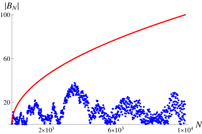
Figure 1: The absolute value of the partial sum $B_{N}=\sum_{n=1}^{N}\cos\left(t\log p_{n}\right)$ versus $N$ for a fixed $t=10^{3}$ (blue dots). The solid red curve is $\sqrt{N}$.

Let us also confirm the gaussian distribution as stated in (17), using the additional freedom that comes from the random variable $u$. It is important to note that $u$ is not chosen independently for each cosine term in the sum; rather one chooses a fixed $u$, randomly, then computes the sum $B_{N}(u)$. In this sense a single sum $B_{N}(u)$ is completely deterministic for a given $u$. Now consider an ensemble $\{B_{N}(u_{i})/\sqrt{N}\}_{i=1}^{E}$, where for each element of the set we choose a random $u_{i}$ in the interval $[0,2\pi]$. Now we can consider its density distribution. In Figure 2 (left) we plot the this density for both $R_{N}/\sqrt{N}$ and $B_{N}/\sqrt{N}$, where $R_{N}$ is given by (16) with $r_{n}$ a random variable on $[-1,1]$. One sees that they are nearly indistinguishable. This is compelling numerical evidence that $B_{N}/\sqrt{N}$ approaches a gaussian distribution at large $N$, with zero mean and variance $1/2$, since $R_{N}/\sqrt{N}$ obeys the CLT with a normal distribution $\tfrac{1}{\sqrt{\pi}}e^{-u^{2}}$. In Figure 2 (right) we can also see that if we use the PNT and replace $p_{n}\approx n\log n$ in (21), we loose this normal distribution. This is expected since with this approximation the $\lambda_{n}$’s will not be linear independent. This shows that the CLT for (21), or (23), comes from fluctuations in the primes, which are not captured by a smooth approximation.

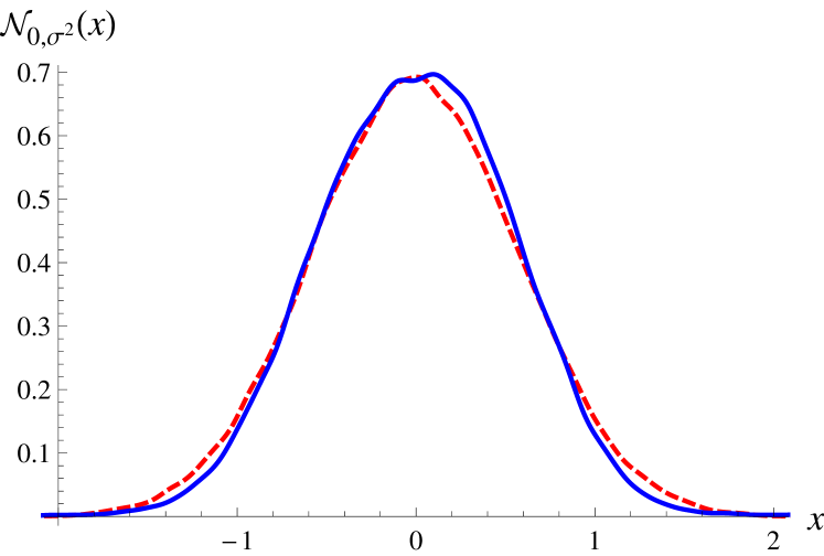
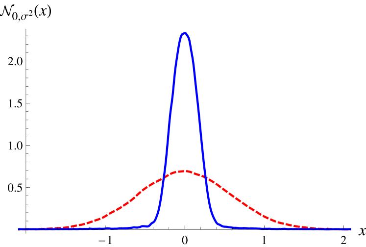
Figure 2: Left: The probability density function of $R_{N}/\sqrt{N}$ (red dashed line) compared with the density of $B_{N}/\sqrt{N}$ (solid blue line). We used $t=10^{3}$, $N=3\cdot 10^{4}$ and $E=8\cdot 10^{4}$ ensembles. Numerically these distributions are a gaussian with variance $\sigma^{2}\approx 0.578$ and approximately zero mean. Right: exactly the same numerical experiment but with the replacement $p_{n}\approx n\log n$ in (21). We clearly see that with this approximation the CLT is no longer valid.

IV Some consequences of the Euler product formula

Having provided analytical arguments and numerical evidence (see Appendix A), in this section we assume the EPF is valid in the sense described above for $\Re(s)>1/2$, and discuss some possible consequences. As already stated in the introduction, one consequence is the validity of the RH, and this extends to the GRH for Dirichlet $L$-functions. For simplicity, we limit this discussion to the $\zeta$-function, however it easily extends, and even more precisely, to the non-principal Dirichlet $L$-functions, since no cut-off $N_{c}$ is required.

IV.1 The function $S(t)$

Let $N(T)$ denote the number of zeros in the entire critical strip, $0<\sigma<1$, up to height $T$, where $T$ is not the ordinate of a zero. There is a known exact formula for $N(T)$ due to Backlund Edwards ,

$$N(T)={1\over\pi}\vartheta(T)+1+S(T),$$ (32)

where $\vartheta(T)$ is the Riemann-Siegel $\vartheta$ function

$$\vartheta(T)=\arg\Gamma(\tfrac{1}{4}+i\,\tfrac{T}{2})-T\log\sqrt{\pi}$$ (33)

and

$$S(T)={1\over\pi}\arg\zeta\left(\tfrac{1}{2}+iT\right).$$ (34)

This result is obtained by the argument principle. Here, $S(T)$ is defined by piecewise integration of $\zeta^{\prime}/\zeta$ from $s=2$, to $2+iT$, then to $1/2+iT$. $N(T)$ is a monotonically increasing staircase function, however it is discontinuous at the ordinates of non-trivial zeros, where it jumps by the multiplicity of the zero. Since $\vartheta(T)$ is smooth, these jumps come from $S(T)$.

Now, if the EPF is valid, then there are no zeros to the right of the critical line. Then $S(T)$ defined by piecewise integration does not encounter any zeros as one approaches the critical line in the piecewise integration, and must be the same as

$$S(T)=\lim_{\delta\to 0^{+}}S_{\delta}(T)$$ (35)

where

$$S_{\delta}(t)\equiv\dfrac{1}{\pi}\arg\zeta\left(\tfrac{1}{2}+\delta+it\right)=-\dfrac{1}{\pi}\lim_{N\to\infty}\Im\left[\sum_{n=1}^{N}\log\left(1-p_{n}^{-1/2-\delta-it}\right)\right].$$ (36)

This is an explicit formula for $S(T)$ expressed as a sum over primes, and for $\delta$ strictly not zero, $S_{\delta}(T)$ is continuous. As explained in FrancaLeclair , $S(t)$ defined by this limiting procedure is also well-defined at the ordinate of a zero on the critical line.

The function $S(T)$ knows about the Riemann zeros since it jumps at each zero. Thus, the expression (32) for $N(T)$, with $S(T)$ replaced by $S_{\delta}(T)$ in (36), which involves a sum over primes, is a relation between Riemann zeros and the primes that is completely the inverse of Riemann’s result for the prime number counting function $\pi(x)$ expressed as a sum over non-trivial zeros. For the latter, one needs to sum over all zeros to identify the primes. Our result is the inverse; to find the zeros, one must sum over all primes. In this sense the distribution of non-trivial zeros on the critical line is explicitly determined by the prime numbers. In Figure 3 we plot equation (32) with $S(T)\to S_{\delta}(T)$, given by (36), with a finite (small) number of primes. The jumps correspond to the nontrivial zeros of $\zeta(s)$. A stronger version of this is presented below; see the discussion following (38). If one replaces $p_{n}\approx n\log n$, then $S_{\delta}(T)$ no longer jumps at the zeros. This indicates that the zeros themselves and their GUE statistics Montgomery ; Odlyzko2 arises from fluctuations in the primes. It would be very interesting to understand the origin of the GUE statistics in this way.

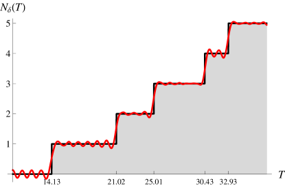
Figure 3: The red line shows a plot of equation (32) with $S(T)$ replaced by $S_{\delta}(T)$ defined in terms of primes in (36), i.e. $N_{\delta}(T)\equiv{1\over\pi}\vartheta(T)+S_{\delta}(T)+1$. Here $\delta=10^{-3}$. We use only $100$ primes in the sum. The solid black line corresponds to the same equation but with the exact $S_{\delta}(T)=\tfrac{1}{\pi}\arg\zeta\left(\tfrac{1}{2}+\delta+iT\right)$. Since $N_{\delta}(T)$ jumps by one at each zero, this indicates that each individual non-trivial zero is related to an infinite sum over primes.

IV.2 A transcendental equation for the $n$-th zero

Let us characterize precisely the zeros on the upper-half of the critical line, $\rho_{n}=\tfrac{1}{2}+it_{n}$ for $n=1,2,3,\dotsc$. In RHLeclair ; FrancaLeclair a transcendental equation for each $t_{n}$ was proposed which depends only on $n$. A more lengthy discussion of this result can be found in our lectures FL3 . This transcendental equation for $t_{n}$ is simple to describe. We are going to consider only the $\zeta(s)$ case to be concise, but the same is easily extended to Dirichlet $L$-functions. Let $\theta(s)=\arg\chi(s)$ where $\chi$ is the completed $\zeta$-function defined in (6). It was argued that the zeros are in one-to-one correspondence to the zeros of $\cos\theta$, namely

$$\lim_{\delta\to 0^{+}}\theta\left(\tfrac{1}{2}+\delta+it_{n}\right)=\left(n-\tfrac{3}{2}\right)\pi.$$ (37)

As explained in FrancaLeclair , if the above equation has a unique solution for every $n$, then the RH is true and all zeros are simple. However, in that work we were unable to prove that this equation has a unique solution for every $n$. As we now describe, the EPF helps to resolve these issues. Let us first provide a different derivation of (37) based on the EPF. Using $S_{\delta}(T)$ in (32), $N(T)$ is now a monotonically increasing staircase function that is smoothed out at the jumps, i.e. it is continuous everywhere (see Figure 3). Since it jumps at the ordinate of a zero $t_{n}$, and the EPF implies there are no zeros off the critical line, one can use $N(T)$ to find an equation for $t_{n}$. Assume for the moment that all zeros are simple. (The derivation of the equation (37) in FrancaLeclair did not assume this.) Then one simply replaces $T\to t_{n}$ and $N\to n-\tfrac{1}{2}$ in $N(T)$:

$$\vartheta\left(t_{n}\right)+\pi\lim_{\delta\to 0^{+}}S_{\delta}\left(t_{n}\right)=\left(n-\tfrac{3}{2}\right)\pi.$$ (38)

This equation is identical to (37). The small $\delta$ is required to be positive because the EPF is only valid to the right of the critical line. The EPF combined with the properties of $N(T)$ implies that the left hand side of the above equation is monotonic and continuous, thus there is a unique solution to (38) for every $n$.

Using the above definition (36) for $S_{\delta}$ in terms of primes, the above equation (38) no longer makes any reference to the $\zeta$-function itself. This indicates that every single individual zero depends on all of the primes. We were actually able to calculate zeros from (38) and (36). For instance, for the $n=10^{5}$, with $N=10^{4}$ primes, we obtained $t_{n}\approx 74920.826$ whereas the actual value is $t_{n}\approx 74920.827$.

The $S_{\delta}(t)$ term in (38) fluctuates and is very small compared with the $\vartheta(t)$ term for large $t$. If one ignores it, and uses Stirling’s approximation for the $\Gamma$-function, then the solution to the resulting equation can be expressed in terms of the Lambert $W$-function FrancaLeclair :

$$t_{n}\approx{2\pi(n-\tfrac{11}{8})\over W[e^{-1}(n-\tfrac{11}{8})]}.$$ (39)

The equation (38) was used to numerically calculate many zeros to very high accuracy, thousands of digits, up to the billion-th zero FrancaLeclair . The approximation (39) is also quite accurate; generally the integer part is correct, but it is smooth and does not capture the fluctuations that satisfy GUE statistics. This is clear since this approximation does not capture any sum over primes. This suggests that the GUE statistics of the zeros originates from the fluctuations of the primes.

As previously stated, the equation (38) is identical to the equation (37) which comes from $\cos\theta=1$. In RHLeclair ; FrancaLeclair the argument which led to (38) was entirely different than the one presented here, i.e. it did not assume the RH nor the simplicity of the zeros, and did not rely on the EPF nor knowledge of $N(T)$. It was obtained directly on the critical line using the functional equation.

The above discussion extends to Dirichlet $L$-functions. The analogs of the above transcendental equations and the Lambert $W$ approximation for Dirichlet $L$-functions, and $L$-functions based on modular forms, were already presented in FrancaLeclair .

IV.3 A Counterexample

A well-known counterexample to the RH is based on the Davenport-Heilbronn function ${\cal D}(s)$, which is a linear combination of two Dirichlet $L$-functions of modulus $k=5$, i.e. $L(s,\chi_{5,2})$ and $L(s,\overline{\chi}_{5,2})$. It satisfies a functional equation like (6). This function is known to have an infinite number of zeros on the critical line, but also has non-trivial zeros off the critical line and inside the critical strip. The Dirichlet $L$-functions each have an Euler product, however the sum does not. The analog of (38) was studied for this function in FrancaLeclair ; FL3 . It was found that the analog of $S_{\delta}(t)$, i.e. $S_{{\cal D}}(t)=\tfrac{1}{\pi}\lim_{\delta\to 0^{+}}\arg{\cal D}\left(\tfrac{1}{2}+\delta+i\,t\right)$, becomes ill-defined in the vicinity of ordinates $t$ corresponding to zeros off of the critical line, and there are no solutions to the analog of (38) at these points. This is now perfectly clear, since there is no Euler product formula to smooth out $S_{\cal D}$ here.

This example provide further evidence that the validity of the RH depends on both the functional equation (6) and the Euler Product Formula (2).

V Conclusions

In this paper we provided arguments that the average, or more specifically the Cesàro average, of the Euler product converges into the right-half part of the critical strip. This implies that the Euler product itself is meaningful in this region. Extensive numerical support for our statements are presented in Appendix A.

The most important, and delicate, argument, is the central limit theorem applied to the random walk of the primes, the series (4). This sum behaves like a normal random variable because of the multiplicative independence of the primes, and the strongly multiplicative property of Dirichlet characters. Furthermore, for non-principal Dirichlet characters, the central limit holds as stated, allowing an arbitrarily large $N$ limit. However, the situation is more subtle for principal Dirichlet $L$-functions, including the $\zeta(s)$ function. In these cases, there is no contribution from the character to (4), and because the gaps between primes get smaller in comparison to the primes, we need to introduce a cut-off, truncating the series (30). However, for large $t$, the cut-off does not impose severe constraints since $N_{c}\sim t^{2}\to\infty$. The cut-off avoids the regime where the cosines sum up constructively. Note that this regime is not due to fluctuations in the primes, but rather the opposite. Furthermore, the cut-off is intimately related to the pole at $s=1$. Our analysis in effect predicts the existence of a pole. Since non-principal Dirichlet $L$-functions have no such a pole, there is no need for a cut-off in this case.

We also discussed some consequences assuming that the Euler product formula is valid for $\Re(s)>1/2$. The most important one, is that the function $S(t)=\tfrac{1}{\pi}\arg\zeta(1/2+\delta+it)$ becomes smooth through the $\delta\to 0^{+}$ limit, and thus we expect the transcendental equation (38) to have a unique solution for every $n$ FrancaLeclair . The same argument applies to Dirichlet $L$-functions, with their respective transcendental equations, also presented in FrancaLeclair .

Appendix A Numerical studies

We have provided arguments that the logarithm of the Euler product Cesàro-converges in the region $\sigma>1/2$, subject to the qualification for principle characters described in the last section. We now present compelling numerical evidence of the validity of this result. Throughout this section we plot the Euler product itself, rather than its average, since the resolution of the plots is not high enough to see the small fluctuations, so that these plots are indistinguishable from the plots of the average. In other words, we provide evidence for the following equality

$$L(s,\chi)=\lim_{N\to\infty}\langle{\cal P}_{N}(s,\chi)\rangle,\qquad{\cal P}_{N}(s,\chi)=\prod_{n=1}^{N}\left(1-\dfrac{\chi(p_{n})}{p_{n}^{\,s}}\right)^{-1},$$ (40)

where $\langle{\cal P}_{N}(s,\chi)\rangle$ is its arithmetic average over $N$:

$$\langle{\cal P}_{N}(s,\chi)\rangle=\dfrac{1}{N}\sum_{n=1}^{N}{\cal P}_{n}(s,\chi).$$ (41)

The above arithmetic average of the product should converge for the same reasons that the arithmetic average of $\log{\cal P}(s,\chi)$ converges, since averaging is just a smoothing procedure.

A.1 Riemann $\zeta$-function

In Figure 4 one can see how the partial product in (40) converges to the $\zeta(s)$ function as we increase $N$. For higher $N$ the curves are indistinguishable. Note, however, that we cannot go beyond the cut-off (30) for a given $t$. Let us also verify convergence for $\arg\zeta$, which plays a central role for the zeros on the critical line (see the Section IV). Using the EPF we have equation (36), whose equality is verified in Figure 5. This assures that both the real and imaginary parts of the Euler product converge. As we approach the critical line $\sigma\to 1/2^{+}$ higher $N$ is of course required.

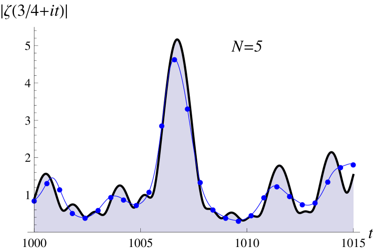
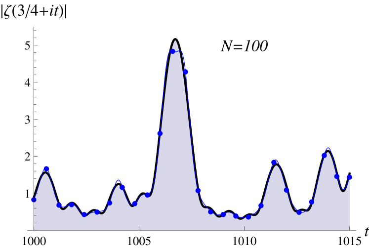
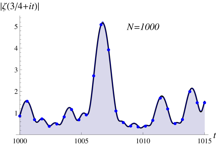
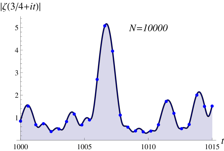
Figure 4: The black line is the actual $|\zeta(3/4+it)|$, analytically continued into the strip, and the blue line is the partial product $|{\cal P}_{N}(3/4+it)|$. Dots are added to the line to aid visualization.

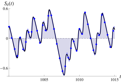
Figure 5: The black line is the actual $\tfrac{1}{\pi}\arg\zeta\left(\tfrac{1}{2}+\delta+it\right)$, and the blue line is the RHS of (36). Dots are added to the line to aid in visualization. We used $\delta=10^{-1}$ and $N=10^{5}$.

One can clearly see how the Euler product formula is not valid for $\sigma\leq 1/2$ from Figure 6. The curves only match for $\sigma>1/2$ and the dramatic change in behavior is abrupt at $\sigma=1/2$, as predicted. The divergences shown in Figure 6 (right) get worse for higher $N$.

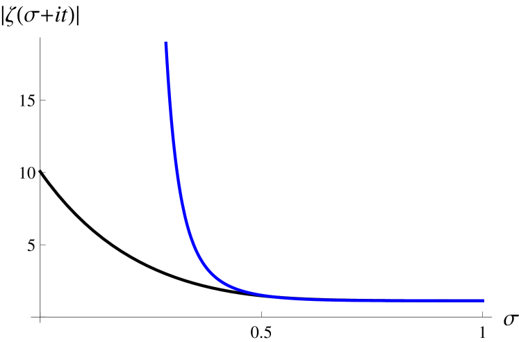
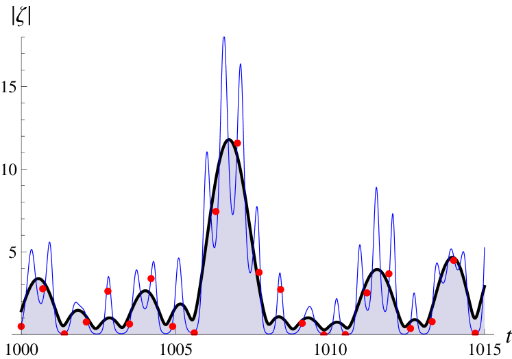
Figure 6: Left: the black line corresponds to $|\zeta(\sigma+it)|$ against $0<\sigma<1$, for $t=500$. The blue line is the partial product $|{\cal P}_{N}(\sigma+it)|$ with $N=10^{4}$. Right: the black line is the exact $|\zeta|$, and the blue line is the partial product $|{\cal P}_{N}|$ (with $N=8\cdot 10^{3}$), against $t$. We took $\sigma=0.4$. The red dots are the Cesàro average $|\langle{\cal P}_{N}\rangle|$. If we increase $N$ the results are even worse.

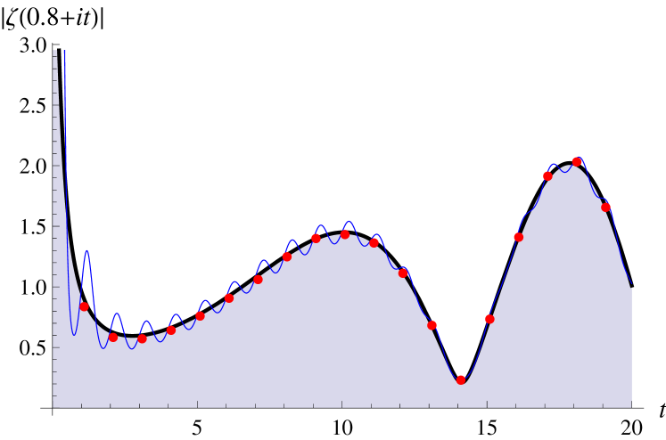
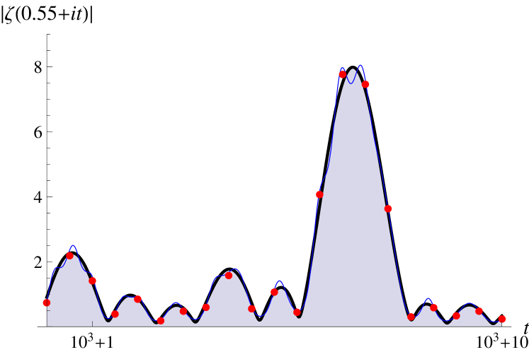
Figure 7: Left: the black line is $|\zeta(0.8+it)|$, and the blue line is $|{\cal P}_{N}|$, with $N=10^{2}$, and the red dots correspond to the Cesàro average $|\langle{\cal P}_{N}\rangle|$. Right: here we have $\zeta(0.55+it)$, and we used $N=4\cdot 10^{4}$. The convergence close to the critical line requires very large $N$.

As we discussed before, there is no convergence on the real line $t=0$ due to the pole at $s=1$. It is exactly because of this divergence that we had to introduce the cut-off (30). However, for short truncations of the product, i.e. not so high $N$, we can describe the $\zeta$-function quite accurately even for low $t$, as shown in Figure 7 (left). We can see that the oscillations get stronger close to $t=0$, but the Cesàro average is still well-behaved and closer to the actual value of $\zeta(s)$ than the partial product itself. The convergence close to the critical line is very slow, and requires very high $N$. Thus to test the results close to the critical line, we also have to choose high $t$ due to the cut-off relation (30). One can see from Figure 7 (right) that the Cesàro average approximates $\zeta(s)$ correctly, even close to the critical line.

In Table 1 we show some values of the average $|\langle{\cal P}_{N}\rangle|$ and the product $|{\cal P}_{N}|$ itself. The convergence is slow, but one can see that $\langle{\cal P}_{N}(s)\rangle\approx\zeta(s)$ as we increase $N$, whereas the unaveraged ${\cal P}_{N}(s)$ continues to oscillate around $\zeta(s)$. With $N=10^{5}$ we obtain nearly $5$ digit accuracy for $t=100$. Note that the results eventually start to get worse for very high $N$, here roughly $10^{8}$. We are increasing $N$ much beyond the cut-off predicted by (30). We can do this since we are not close to the critical line.

$N$	$|\langle{\cal P}_{N}\rangle|$	$|{\cal P}_{N}|$
$1\cdot 10^{3}$	$0.976752$	$0.972210$
$2\cdot 10^{3}$	$0.976690$	$0.981506$
$3\cdot 10^{3}$	$0.977653$	$0.976654$
$4\cdot 10^{3}$	$0.977865$	$0.975735$
$5\cdot 10^{3}$	$0.977926$	$0.984674$
$6\cdot 10^{3}$	$0.977463$	$0.977893$
$7\cdot 10^{3}$	$0.978208$	$0.976510$
$8\cdot 10^{3}$	$0.977593$	$0.978773$
$9\cdot 10^{3}$	$0.978290$	$0.981781$
$1\cdot 10^{4}$	$0.977900$	$0.971017$
$1\cdot 10^{5}$	$0.977703$	$0.971203$
$1\cdot 10^{6}$	$0.977925$	$0.971491$
$1\cdot 10^{7}$	$0.978168$	$0.978027$
$1\cdot 10^{8}$	$0.977823$	$0.984481$
$2\cdot 10^{8}$	$0.956304$	$0.885545$
$3\cdot 10^{8}$	$0.924928$	$0.794254$
$|\zeta(0.95+i\,20)|=0.977848$

$N$	$|\langle{\cal P}_{N}\rangle|$	$|{\cal P}_{N}|$
$1\cdot 10^{3}$	$1.690988$	$1.694894$
$2\cdot 10^{3}$	$1.692350$	$1.694156$
$3\cdot 10^{3}$	$1.692590$	$1.690354$
$4\cdot 10^{3}$	$1.692399$	$1.688480$
$5\cdot 10^{3}$	$1.691996$	$1.687150$
$6\cdot 10^{3}$	$1.691666$	$1.689158$
$7\cdot 10^{3}$	$1.691508$	$1.688145$
$8\cdot 10^{3}$	$1.691400$	$1.691700$
$9\cdot 10^{3}$	$1.691381$	$1.692973$
$1\cdot 10^{4}$	$1.691345$	$1.690480$
$1\cdot 10^{5}$	$1.691373$	$1.692136$
$1\cdot 10^{6}$	$1.691429$	$1.691577$
$1\cdot 10^{7}$	$1.691414$	$1.691703$
$1\cdot 10^{8}$	$1.691385$	$1.693287$
$2\cdot 10^{8}$	$1.745257$	$1.923738$
$3\cdot 10^{8}$	$1.852499$	$2.203470$
$|\zeta(0.95+i\,100)|=1.691397$

Table 1: Convergence $\langle{\cal P}_{N}\rangle$, and ${\cal P}_{N}$, for the $\zeta$-function. Note that even for $N\gg N_{c}\sim t^{2}$ the results are good, but eventually it starts to deviate from the correct value as shown in the two last entries.

A.2 Non-principle Dirichlet $L$-functions

Let us consider a concrete example with the primitive character of modulus $7$, shown below:

$$n$$

(42)

In Figure 8 (left) we plot the absolute value of the partial Euler product for $L(s,\chi_{7,2})$, and we can see how it fits the $L$-function on the right-half part of the critical strip, even at the real line $t=0$, since there is no pole. This is in clear contrast with Figure 7 where the Euler product for $\zeta(s)$ is not even finite on the line segment $1/2<s\leq 1$. Thus one clearly sees that $\zeta(s)$ is exceptional, along with the other principal Dirichlet $L$-functions. The convergence of the Euler product for non-principal Dirichlet $L$-functions is much better behaved. In fact one may check that the analog of Figure 1 has smaller fluctuations and resembles even more the standard random walk. As explained, in this case there is no cut-off $N_{c}$, and we can take $N$ as large as desirable. In Figure 8 (right) we see the Cesàro average in comparison with the actual value of $L(s,\chi_{7,2})$, closer to the critical line.

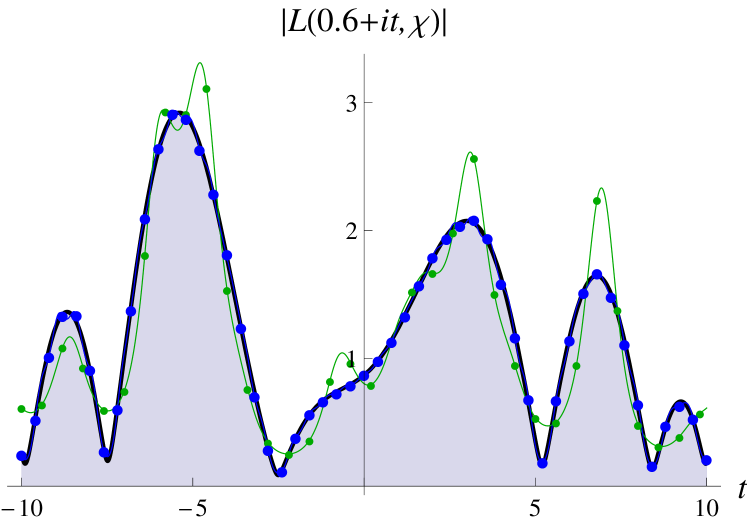
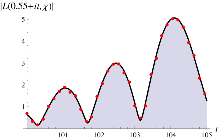
Figure 8: Left: we have $s=0.6+it$. The black line is $|L(s,\chi)|$ with $\chi=\chi_{7,2}$ given in (42). The green line is the partial product $|{\cal P}_{N}(s,\chi)|$ obtained with only $N=5$, while the blue line with $N=10^{4}$. We can see that the results get better as we increase $N$. We can also see that there are no divergences on the real line $t=0$, in contrast with Figure 7. Right: here we are closer to the critical line, $s=0.55+it$. The black line is $|L(s,\chi)|$, and the red dots correspond to the Cesàro average $|\langle{\cal P}_{N}(s,\chi)\rangle|$ with $N=5\cdot 10^{6}$.

In Table 2 we compute the partial product, and its Cesàro average, for $L(s,\chi_{7,2})$. We can see how the last digits fluctuate but the numbers are close to the actual value of $|L(s,\chi_{7,2})|$. Note that, contrary to the $\zeta(s)$ case where we are limited in accuracy by the cut-off $N\leq N_{c}$, for non-principal Dirichlet $L$-functions we expect the results to get better and better as we arbitrarily increase $N$.

$N$	$|\langle{\cal P}_{N}\rangle|$	$|{\cal P}_{N}|$
$1\cdot 10^{3}$	$0.8940791$	$0.8949042$
$2\cdot 10^{3}$	$0.8947639$	$0.8951913$
$3\cdot 10^{3}$	$0.8948319$	$0.8946522$
$4\cdot 10^{3}$	$0.8947869$	$0.8950135$
$5\cdot 10^{3}$	$0.8948144$	$0.8946950$
$6\cdot 10^{3}$	$0.8947834$	$0.8945271$
$7\cdot 10^{3}$	$0.8947674$	$0.8948700$
$8\cdot 10^{3}$	$0.8947783$	$0.8947044$
$9\cdot 10^{3}$	$0.8947768$	$0.8948476$
$1\cdot 10^{4}$	$0.8947921$	$0.8950163$
$1\cdot 10^{5}$	$0.8949043$	$0.8949518$
$|L\left(0.95,\chi\right)|=0.89492570$

$N$	$|\langle{\cal P}_{N}\rangle|$	$|{\cal P}_{N}|$
$1\cdot 10^{3}$	$0.6183514$	$0.6208759$
$2\cdot 10^{3}$	$0.6195137$	$0.6202016$
$3\cdot 10^{3}$	$0.6199206$	$0.6211404$
$4\cdot 10^{3}$	$0.6201229$	$0.6205615$
$5\cdot 10^{3}$	$0.6202306$	$0.6207769$
$6\cdot 10^{3}$	$0.6202884$	$0.6205089$
$7\cdot 10^{3}$	$0.6203365$	$0.6207366$
$8\cdot 10^{3}$	$0.6203860$	$0.6207027$
$9\cdot 10^{3}$	$0.6204248$	$0.6207634$
$1\cdot 10^{4}$	$0.6204524$	$0.6207338$
$1\cdot 10^{5}$	$0.6207878$	$0.6209509$
$|L\left(0.95+i\,100,\chi\right)|=0.62101132$

Table 2: Numerical results for the Euler product and its Cesàro average for $\chi=\chi_{7,2}$, shown in (42). We expect the results to be more accurate as we increase $N$. We choose $t=0$ in the left table to explicitly show that there are no divergences on the real line.

References

- (1) B. Riemann. Ueber die Anzahl der Primzahlen unter einer gegebenen Grösse. Monatsberichte der Berliner Akademie. In Gesammelte Werke, Teubner, Leipzig, 1982.
- (2) M. V. Berry and J. P. Keating. The Riemann Zeros and Eigenvalue Asymptotics. SIAM Rev., 41(2):236–266, 1999.
- (3) S. M. Gonek, C. P. Hughes, and J. P. Keating. A Hybrid Euler-Hadamard product formula for the Riemann zeta function. Duke Math. J, 136(3):507–549, 2007.
- (4) E. C. Titchmarsh. The Theory of the Riemann Zeta-Function. Oxford University Press, ”New York”, 1988.
- (5) H. M. Bui and J. P. Keating. On the Mean Values of Dirichlet -functions. Proc. London Math. Soc., 95(3):273–298, 2007.
- (6) H. M. Bui and J. P. Keating. On the Mean Values of -functions in Orthogonal and Symplectic Families. Proc. London Math. Soc., 96(3):335–366, 2008.
- (7) S. M. Gonek and J. P. Keating. Mean Values of Finite Euler Products. Proc. London Math. Soc., 82(2):763–786, 2010.
- (8) S. M. Gonek. Finite Euler products and the Riemann hypothesis. Trans. Amer. Math. Soc., 364(4):2157–2191, 2011.
- (9) K. Conrad. Partial Euler products on the critical line. Canad. J. Math., 57:267–297, 2005.
- (10) T. Kimura, S.-Y. Koyama, and N. Kurokawa. Euler products beyond the boundary. Lett. Math. Phys., 104:1–19, 2014.
- (11) T. Tao. Structure and randomness in the prime numbers. In Dierk Schleicher and Malte Lackmann, editors, An Invitation to Mathematics, pages 1–7. Springer-Verlag, Berlin Heidelberg, 2011.
- (12) G. H. Hardy. Divergent Series. American Mathematical Society, New York, 1992.
- (13) A. LeClair. An electrostatic depiction of the validity of the Riemann hypothesis and a formula for the -th zero at large . Int. J. Mod. Phys. A, 28(30):1350151, 2013. arXiv:1305.2613 [math-ph].
- (14) G. França and A. LeClair. Transcendental equations satisfied by the individual zeros of Riemann , Dirichlet and modular -functions. Comm. Number Theory and Phys., 9(1):1–49, 2015. arXiv:1502.06003v1 [math.NT], arXiv:1307.8395 [math.NT] and arXiv:1309.7019 [math.NT].
- (15) P. R. Chernoff. A pseudo zeta function and the distribution of primes. PNAS, 97(14):7697–7699, 2000.
- (16) R. Salem and A. Zygmund. On lacunary trigonometric series. PNAS, 33(11):333–338, 1947.
- (17) R. Salem and A. Zygmund. On lacunary trigonometric series, II. PNAS, 34(2):54–62, 1948.
- (18) M. Kac. Statistical Independence in Probability, Analysis and Number Theory. The Mathematical Association of America, New Jersey, 1959.
- (19) P. Billingsley. Convergence of Probability Measures. John Wiley & Sons, Inc., New York, 1999.
- (20) P. Billingsley. Probability and Measure. John Wiley & Sons, Inc., New York, 1995.
- (21) C-E. Fröberg. On the Prime Zeta Function. Nordisk Tidskr. Informationsbehandling (BIT), 8(3):187–202, 1968.
- (22) E. Muñoz García and R. Pérez Marco. The Product Over All Primes is . Commun. Math. Phys, 277(1):69–81, 2008.
- (23) H. M. Edwards. Riemann’s Zeta Function. Dover Publications Inc., Mineola, New York, 1974.
- (24) H. Montgomery. The pair correlation of zeros of the zeta function. In Analytic number theory, Proc. Sympos. Pure Math. XXIV, page 181D193, Providence, R.I.: AMS, 1973.
- (25) A. M. Odlyzko. On the distribution of spacings between zeros of the zeta function. Math. Comp., 48:273–308, 1987.
- (26) G. França and A. LeClair. A theory for the zeros of Riemann Zeta and other -functions. Lectures delivered by A. LeClair at “Riemann Master School on Zeta Functions” at Leibniz Universität, Hannover, Germany, June 10-14, arXiv:1407.4358 [math.NT], 2014.