Abstract

We consider the task of fitting a regression model involving interactions among a potentially large set of covariates, in which we wish to enforce strong heredity. We propose FAMILY, a very general framework for this task. Our proposal is a generalization of several existing methods, such as VANISH (Radchenko and James, 2010), hierNet (Bien et al., 2013), the all-pairs lasso, and the lasso using only main effects. It can be formulated as the solution to a convex optimization problem, which we solve using an efficient alternating directions method of multipliers (ADMM) algorithm. This algorithm has guaranteed convergence to the global optimum, can be easily specialized to any convex penalty function of interest, and allows for a straightforward extension to the setting of generalized linear models. We derive an unbiased estimator of the degrees of freedom of FAMILY, and explore its performance in a simulation study and on an HIV sequence data set.

1 Introduction

1.1 Modeling Interactions

In this paper, we model a response variable with a set of main effects and second-order interactions. The problem can be formulated as follows: we are given a response vector $y$ for $n$ observations, an $n\times p_{1}$ matrix $X$ of covariates and another $n\times p_{2}$ matrix $Z$ of covariates. In what follows, the notation $X_{.,j}$ and $Z_{.,k}$ will denote the $j^{th}$ column of $X$ and $k^{th}$ column of Z, respectively. The goal is to fit the model

$$y_{i}=B_{0,0}+\sum_{j=1}^{p_{1}}B_{j,0}X_{i,j}+\sum_{k=1}^{p_{2}}B_{0,k}Z_{i,k}+\sum_{j=1}^{p_{1}}\sum_{k=1}^{p_{2}}B_{j,k}X_{i,j}Z_{i,k}+\varepsilon_{i},\ \ i=1,\ldots,n,$$ (1)

where $B$ is a $(p_{1}+1)\times(p_{2}+1)$ matrix of coefficients, of which the rows and columns are indexed from 0 to $p_{1}$ and 0 to $p_{2}$ for the variables $X$ and $Z$, respectively. In the special case where $X=Z$, the coefficient of the $(j,k)^{th}$ interaction is $B_{j,k}+B_{k,j}$, and the coefficient of the $j^{th}$ main effect is $B_{0,j}+B_{j,0}$.

For brevity, we re-write model (1) using array notation. We construct the $n\times(p_{1}+1)\times(p_{2}+1)$ array $W$ as follows: for $i\in\{1,\ldots,n\},j\in\{0,\ldots,p_{1}\},k\in\{0,\ldots,p_{2}\},$

$$W_{i,j,k}=\begin{cases}X_{i,j}Z_{i,k}&\mbox{ for }j\not=0\mbox{ and }k\not=0\\ X_{i,j}&\mbox{ for }k=0\mbox{ and }j\not=0\\ Z_{i,k}&\mbox{ for }j=0\mbox{ and }k\not=0\\ 1&\mbox{ for }j=k=0\end{cases}.$$ (2)

Then (1) is equivalent to the model

$$y=W*B+\varepsilon,$$ (3)

where $B$ is the matrix of coefficients as in (1), and $W*B$ denotes the $n$-vector whose $i^{th}$ element takes the form $(W*B)_{i}\equiv\sum_{j=0}^{p_{1}}\sum_{k=0}^{p_{2}}W_{i,j,k}B_{j,k}$. The model is displayed in the left panel of Figure 1.

In fitting models with interactions, we may wish to impose either strong or weak heredity (Hamada and Wu, 1992; Yates, 1978; Chipman, 1996; Joseph, 2006), defined as follows:

• Strong Heredity: If an interaction term is included in the model, then both of the corresponding main effects must be present. That is, if $B_{j,k}\not=0$, then $B_{j,0}\not=0$ and $B_{0,k}\not=0$.

• Weak Heredity: If an interaction term is included in the model, then at least one of the corresponding main effects must be present. That is, if $B_{j,k}\not=0$, then either $B_{j,0}\not=0$ or $B_{0,k}\not=0$.

Such constraints facilitate model interpretation (McCullagh, 1984), improve statistical power (Cox, 1984), and simplify experimental designs (Bien et al., 2013). In this paper we propose a general convex regularized regression approach which naturally and efficiently enforces strong heredity.

1.2 Summary of Previous Work

A number of authors have considered the task of fitting interaction models under strong or weak heredity constraints. Constraints to enforce heredity (Peixoto, 1987; Friedman, 1991; Bickel et al., 2010; Park and Hastie, 2008; Wu et al., 2010) have been applied to conventional step-wise model selection techniques (Montgomery et al., 2012, chap. 10). Chipman (1996) and George and McCulloch (1993) proposed Bayesian methods. In more recent work, Hao and Zhang (2014) proposed iFORM, an approach that performs forward selection on the main effects, and allows interactions into the model once the main effects have already been selected. iFORM  has a number of attractive properties, including suitability for the ultra-high-dimensional setting, computational efficiency, as well as proven theoretical guarantees.

In this paper, we take a regularization approach to inducing strong heredity. A number of regularization approaches for this task have already been proposed in the literature; in fact, a strength of our proposal is that it provides a unified framework (and associated algorithm) of which several existing approaches can be seen as special cases. Choi et al. (2010) propose a non-convex approach, which amounts to a lasso (Tibshirani, 1996) problem with re-parametrized coefficients. Alternatively, some authors have enforced strong or weak heredity via convex penalties or constraints. Jenatton et al. (2011) and Zhao et al. (2009) describe a set of penalties that can be applied to a broad class of problems. As a special case they consider interaction models with strong or weak heredity; this has been further developed by Bach et al. (2012). Radchenko and James (2010), Lim and Hastie (2013) and Bien et al. (2013) propose penalties specifically designed for interaction models with sparsity and strong heredity. We now describe the latter two approaches in greater detail.

1.2.1 hierNet (Bien et al., 2013)

The hierNet approach of Bien et al. (2013) fits the model (1) with $X=Z$ and $p_{1}=p_{2}=p$. In the case of strong heredity, using the notation of (3), they consider the problem

$$\begin{split}\underset{B\in\mathbb{R}^{(p+1)\times(p+1)},\ \beta^{\pm}\in\mathbb{R}^{p}}{\text{minimize}}\ &\frac{1}{2}\|y-W*B\|_{2}^{2}+\lambda\sum_{j=1}^{p}(\beta_{j}^{+}+\beta_{j}^{-})+\frac{\lambda}{2}\|B_{-0,-0}\|_{1}\\ \text{subject to }&B=B^{T},\ B_{0,-0}=\beta^{+}-\beta^{-}\\ &\|B_{j,-0}\|_{1}\leq\beta_{j}^{+}+\beta_{j}^{-},\ \beta_{j}^{+}\geq 0,\beta_{j}^{-}\geq 0\text{ for }j=1,\ldots,p.\end{split}$$ (4)

Using this notation, the coefficient for the $j^{th}$ main effect is ${B}_{0,j}+{B}_{j,0}$, and the coefficient for the $(j,k)^{th}$ interaction is ${B}_{j,k}+{B}_{k,j}$. Strong heredity is imposed by the constraint $\|B_{j,-0}\|_{1}\leq\beta_{j}^{+}+\beta_{j}^{-}$.

1.2.2 glinternet (Lim and Hastie, 2013)

Like hierNet, the glinternet proposal of Lim and Hastie (2013) fits (1) with $X=Z$ and $p_{1}=p_{2}=p$. In order to describe this approach, we introduce some additional notation. Let $\alpha_{k}$ be the coefficient of the $k^{th}$ main effect. We decompose $\alpha_{k}$ into $p$ parameters, i.e. $\alpha_{k}=\alpha_{k}^{(0)}+\alpha_{k}^{(1)}+\ldots+\alpha_{k}^{(k-1)}+\alpha_{k}^{(k+1)}+\ldots+\alpha_{k}^{(p)}$. We let $\alpha_{jk}+\alpha_{kj}$ denote the coefficient for the interaction between $X_{j}$ and $X_{k}$. Lim and Hastie (2013) propose to solve the optimization problem

$$\begin{split}\underset{\parbox{115.63243pt}{ $\alpha_{0},\{\alpha_{ij}\}_{i\not=j;i,j\not=0},\\ \{\alpha_{i}^{(j)}\}_{j\not=i}\in\mathbb{R}$ }}{\text{minimize}}&\left\|y-\alpha_{0}-\sum_{k=1}^{p}\sum_{j\not=k}\alpha_{k}^{(j)}X_{.,k}-\sum_{j\not=k}\alpha_{jk}\left(X_{.,j}*X_{.,k}\right)\right\|_{2}^{2}\\ &+\lambda\left(\sum_{j=1}^{p}|\alpha^{(0)}_{j}|+\sum_{j\neq k}\sqrt{\left(\alpha_{j}^{(k)}\right)^{2}+\left(\alpha_{k}^{(j)}\right)^{2}+\alpha^{2}_{jk}}\right),\end{split}$$ (5)

where $X_{.,j}*X_{.,k}$ denotes element-wise multiplication. Strong heredity is enforced via the group lasso (Yuan and Lin, 2006) penalties: if either $\alpha_{jk}$ or $\alpha_{kj}$ is estimated as non-zero, then $\alpha_{j}^{(k)}$ and $\alpha_{k}^{(j)}$ will be estimated to be non-zero, and hence so will $\alpha_{j}$ and $\alpha_{k}$.

1.3 Organization of Paper

The rest of this paper is organized as follows. In Section 2, we provide details of FAMILY, our proposed approach for modeling interactions. An unbiased estimator for its degrees of freedom is in Section 3, and an extension to weak heredity is in Section 4. We explore FAMILY’s empirical performance in simulation in Section 5, and in an application to an HIV data set in Section 6. The Discussion is in Section 7.

2 Modeling Interactions with FAMILY

We propose a framework for modeling interactions with a convex penalty (FAMILY). The FAMILY  approach is the solution to a convex optimization problem, which (using the notation of Section 1.1) takes the form

$$\begin{split}\underset{B\in\mathbb{R}^{(p_{1}+1)\times(p_{2}+1)}}{\text{minimize}}\frac{1}{2n}\|y-W*B\|_{2}^{2}+\lambda_{1}\sum_{j=1}^{p_{1}}P_{r}(B_{j,.})+\lambda_{2}\sum_{k=1}^{p_{2}}P_{c}(B_{.,k})+\lambda_{3}\|B_{-0,-0}\|_{1}.\end{split}$$ (6)

Here, $\lambda_{1}$, $\lambda_{2}$, and $\lambda_{3}$ are non-negative tuning parameters. $P_{r}$ and $P_{c}$ are convex penalty functions on the rows and columns of the coefficient matrix $B$. The $\|B_{-0,-0}\|_{1}$ term denotes the element-wise $\ell_{1}$-norm on the interactions, which enforces sparsity on the interaction coefficients when $\lambda_{3}$ is large. The right panel of Figure 1 demonstrates the action of each penalty on the matrix $B$.

As we will see, the choice of $P_{r}$ and $P_{c}$ will determine the type of structure (such as strong heredity) enforced on the fitted model. In the examples that follow, we take $P_{r}=P_{c}$; however, in principle, these two penalty functions need not be equal. For instance, if the features in $Z$ are known to be of scientific importance, we might choose to perform feature selection on the main effects of $X$ only. In this case, we might choose to use $P_{r}(b)=\|b\|_{2}$ and $P_{c}(b)=0$.

We suggest standardizing the columns of $X$ and $Z$ to have mean zero and variance one before solving (6), in order to ensure that the main effects and interactions are on the same scale, as is standard practice for penalized regression estimators (Hastie et al., 2009). We take this approach in Sections 5 and 6.

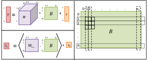
Figure 1: Left: The model (1), for all $n$ observations (top) and for the $i^{th}$ observation (bottom). The notation $\langle W_{i,\cdot,\cdot},B\rangle$ denotes the inner product, $\sum_{j,k}W_{i,j,k}B_{j,k}$. Right: In (6), the $(p_{1}+1)\times(p_{2}+1)$ coefficient matrix $B$ is penalized by applying the $P_{r}$ and $P_{c}$ penalties to each of the $p_{1}$ rows () and each of the $p_{2}$ columns (), respectively. The $\ell_{1}$ penalty is applied to each of the $p_{1}p_{2}$ interactions ().

2.1 Connections to Lasso (Tibshirani, 1996)

The main effects lasso can be viewed as a special case of (6) where $P_{c}$ and $P_{r}$ are $\ell_{1}$ penalties,

$$\begin{split}\underset{B\in\mathbb{R}^{(p_{1}+1)\times(p_{2}+1)}}{\text{minimize}}&\frac{1}{2n}\|y-W*B\|_{2}^{2}+\lambda_{1}\sum_{j=1}^{p_{1}}\|B_{j,.}\|_{1}+\lambda_{2}\sum_{k=1}^{p_{2}}\|B_{.,k}\|_{1}+\lambda_{3}\|B_{-0,-0}\|_{1},\end{split}$$ (7)

and where $\lambda_{3}$ is chosen sufficiently large as to shrink all of the interaction terms to 0. In this case, the lasso penalties on the rows and columns are applied only to the main effects.

In contrast, if we take $\lambda_{3}=0$, $\lambda_{1}=\lambda_{2}=\lambda$, and $P_{c}(b)=P_{r}(b)=|b_{1}|+1/2\|b_{-1}\|_{1}$, where $b=(b_{1},b_{-1}^{T})^{T}$, then (6) yields the all-pairs lasso, which applies a lasso penalty to all main effects and all interactions. In this case, (6) can be re-written more simply as

$$\begin{split}\underset{B\in\mathbb{R}^{(p_{1}+1)\times(p_{2}+1)}}{\text{minimize}}\frac{1}{2n}\|y-W*B\|_{2}^{2}&+\lambda\|B\|_{1}.\end{split}$$ (8)

However, our main interest in this paper is to develop a convex framework for modeling interactions that obeys strong heredity. Clearly, the all-pairs lasso does not satisfy strong heredity, and the main effects lasso does so only in a trivial way (by setting all interaction coefficient estimates to zero).

2.2 FAMILY with Strong Heredity

We now consider three choices of $P_{r}$ and $P_{c}$ in (6) that yield an estimator that obeys strong heredity. In Section 2.2.1, we consider the case where $P_{r}$ and $P_{c}$ are group lasso penalties. In Section 2.2.2, we consider the case where they are $\ell_{\infty}$ penalties. We consider a hybrid between an $\ell_{1}$ and an $\ell_{\infty}$ norm in Section 2.2.3. The unit norm balls corresponding to these three penalties are displayed in Figure 2.

2.2.1 FAMILY with an $\ell_{2}$ Penalty

We first consider (6) in the case where $P_{r}(b)=P_{c}(b)=\|b\|_{2}$, which we will refer to as FAMILY.l2. The resulting optimization problem takes the form

$$\underset{B\in\mathbb{R}^{(p_{1}+1)\times(p_{2}+1)}}{\text{minimize}}\frac{1}{2n}\|y-W*B\|_{2}^{2}+\lambda_{1}\sum_{j=1}^{p_{1}}\|B_{j,.}\|_{2}+\lambda_{2}\sum_{k=1}^{p_{2}}\|B_{.,k}\|_{2}+\lambda_{3}\|B_{-0,-0}\|_{1}.$$ (9)

This formulation will induce strong heredity, in the sense that an interaction between $X_{j}$ and $X_{k}$ can have a non-zero coefficient estimate only if both of the corresponding main effects are non-zero.

Problem 9 is closely related to VANISH, an approach for non-linear interaction modeling (Radchenko and James, 2010). In fact, if we take $X=Z$ and assume that all main effects and interactions are scaled to have norm one in (9), and consider the case of VANISH with only linear main effects and interactions, then VANISH and (9) coincide exactly.

Radchenko and James (2010) attempt to solve the VANISH optimization problem via block coordinate descent. However, due to non-separability of the groups, their algorithm is not guaranteed convergence to the global optimum. In contrast, the algorithm in Section 2.3 is guaranteed convergence to the global optimum of (6) for any convex penalty, and can be extended to the case of generalized linear models.

2.2.2 FAMILY with an $\ell_{\infty}$ Penalty

We now consider (6) in the case where $P_{r}(b)=P_{c}(b)=\|b\|_{\infty}$; we refer to this in what follows as FAMILY.linf. We refer the reader to Duchi and Singer (2009) for a discussion of the properties of the $\ell_{\infty}$ norm, and its merits relative to the $\ell_{2}$ norm in inducing group sparsity. In this case, (6) takes the form

$$\underset{B\in\mathbb{R}^{(p_{1}+1)\times(p_{2}+1)}}{\text{minimize}}\frac{1}{2n}\|y-W*B\|_{2}^{2}+\lambda_{1}\sum_{j=1}^{p_{1}}\|B_{j,.}\|_{\infty}+\lambda_{2}\sum_{k=1}^{p_{2}}\|B_{.,k}\|_{\infty}+\lambda_{3}\|B_{-0,-0}\|_{1}.$$ (10)

This formulation also induces strong heredity.

2.2.3 FAMILY with a Hybrid $\ell_{1}$/$\ell_{\infty}$ Penalty

Finally, we consider (6) with $P_{r}(b)=P_{c}(b)=\max(|b_{1}|,\|b_{-1}\|_{1})$. In this case, (6) takes the form

$$\small\underset{B\in\mathbb{R}^{(p_{1}+1)\times(p_{2}+1)}}{\text{minimize}}\frac{1}{2n}\|y-W*B\|_{2}^{2}+\lambda_{1}\sum_{j=1}^{p_{1}}\max(|B_{j,0}|,\|B_{j,-0}\|_{1})+\lambda_{2}\sum_{k=1}^{p_{2}}\max(|B_{0,k}|,\|B_{-0,k}\|_{1})+\lambda_{3}\|B_{-0,-0}\|_{1}.$$ (11)

In the special case where $X=Z$, $\lambda_{1}=\lambda_{2}=\lambda$, and $\lambda_{3}=\lambda/2$, (11) is in fact equivalent to the hierNet proposal of Bien et al. (2013). Details of this equivalence are given in Bien et al. (2013).

Bien et al. (2013) propose to solve hierNet via an ADMM algorithm which applies a generalized gradient descent loop within each update. This leads to computational inefficiency, especially for large $p$. In Section 2.3, we propose a simple, stand-alone ADMM algorithm for solving (6), which can be easily applied to solve (11), and consequently also the hierNet optimization problem.

Given its connection to Bien et al. (2013), we refer to (11) as FAMILY.hierNet.

2.2.4 Dual Norms

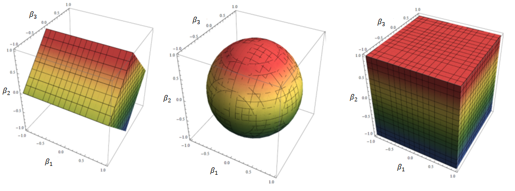
Figure 2: A graphical representation of the region $P(\beta)\leq 1$, where $P(\beta)=\max\left(|\beta_{1}|,|\beta_{2}|+|\beta_{3}|\right)$ (left); $P(\beta)=\sqrt{\beta_{1}^{2}+\beta_{2}^{2}+\beta_{3}^{2}}$ (center); or $P(\beta)=\max(|\beta_{1}|,|\beta_{2}|,|\beta_{3}|)$ (right).

Here we further consider the $l_{2},\ l_{\infty}$ and $l_{1}/l_{\infty}$ hybrid penalties discussed in Sections 2.2.1-2.2.3. For an arbitrary penalty, the proximal operator is the solution to the optimization problem

$$\underset{\beta}{\text{minimize}}\ \ \frac{1}{2}\|y-\beta\|^{2}+\lambda P(\beta).$$ (12)

We begin by presenting a well-known lemma (see e.g. Proposition 1.1, Bach et al. (2011)).

Lemma 2.1.

Let $P(y)$ be a norm of $y$ with dual norm $P_{*}(y)\equiv\max_{z}\ \{z^{T}y:P(z)\leq 1\}$. Then $\hat{\beta}=0$ solves (12) if and only if $P_{*}(y)\leq\lambda$.

It is well-known that the $\ell_{2}$ norm is its own dual norm, and that the $\ell_{1}$ norm is dual to the $\ell_{\infty}$ norm. We now derive the dual norm for the FAMILY.hierNet penalty. This lemma is proven in Appendix B.

Lemma 2.2.

The dual norm of $P(\beta)=\max\{|\beta_{1}|,\|\beta_{-1}\|_{1}\}$ takes the form

$$P_{*}(\beta)=|\beta_{1}|+\|\beta_{-1}\|_{\infty}.$$ (13)

Lemmas 2.1 and 2.2 provide insight into the values of $y$ for which all variables are shrunken to zero in (12). The dual norm balls for the hybrid $\ell_{1}$/$\ell_{\infty}$, $\ell_{2}$, and $\ell_{\infty}$ norms are displayed in Figure 3. By Lemma 2.1, any $y$ inside the dual norm ball leads to a zero solution of (12). For the hybrid $\ell_{1}$/$\ell_{\infty}$ norm, the shape of the dual norm ball implies that the first element of $y$ plays an outsize role in whether or not the coefficient vector is shrunken to zero. Consequently, the main effects play a larger role than the interactions in determining whether sparsity is induced. In contrast, for the $\ell_{\infty}$ and $\ell_{2}$ norms, the main effect and interactions play an equal role in determining whether the coefficients are shrunken to zero.

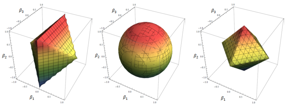
Figure 3: A graphical representation of the region $P_{*}(\beta)\leq 1$, where $P_{*}(\beta)$ is the dual norm for $P(\beta)=\max\left(|\beta_{1}|,|\beta_{2}|+|\beta_{3}|\right)$ (left); $P(\beta)=\sqrt{\beta_{1}^{2}+\beta_{2}^{2}+\beta_{3}^{2}}$ (center); or $P(\beta)=\max(|\beta_{1}|,|\beta_{2}|,|\beta_{3}|)$ (right).

2.3 Algorithm for Solving FAMILY

A step-by-step ADMM algorithm for solving FAMILY is provided in Appendix A.2. Here, we present an overview of this algorithm. A gentle introduction to ADMM is provided in Appendix A.1.

2.3.1 ADMM Algorithm for Solving FAMILY

We now develop an ADMM algorithm to solve (6). We define the variable $\Theta=(D|E|F)$, with $D,E,F\in\mathbb{R}^{(p_{1}+1)\times(p_{2}+1)}$. That is, $\Theta$ is a $(p_{1}+1)\times 3(p_{2}+1)$ matrix, which we partition into $D,\ E$, and $F$ for convenience. Then (6) can be re-written as

$$\underset{\parbox{108.405pt}{ $B\in\mathbb{R}^{(p_{1}+1)\times(p_{2}+1)},\\ \Theta\in\mathbb{R}^{(p_{1}+1)\times 3(p_{2}+1)}$ }}{\text{minimize }}\left\{\frac{1}{2n}\|{y}-{W}*B\|_{2}^{2}+\lambda_{1}\sum_{j=1}^{p_{1}}P_{r}(D_{j,.})+\lambda_{2}\sum_{k=1}^{p_{2}}P_{c}(E_{.,k})+\lambda_{3}\|F_{-0,-0}\|_{1}\right\}$$

$$\mathrm{subject\;to\;}\qquad B(I_{(p_{2}+1)\times(p_{2}+1)}|I_{(p_{2}+1)\times(p_{2}+1)}|I_{(p_{2}+1)\times(p_{2}+1)})=\Theta.$$ (14)

The augmented Lagrangian corresponding to (14) takes the form

$$\small\begin{split}L_{\rho}(B,\Theta,\Gamma)&=\frac{1}{2n}\|{y}-{W}*B\|_{2}^{2}+\lambda_{1}\sum_{j=1}^{p_{1}}P_{r}({D}_{j,.})+\lambda_{2}\sum_{k=1}^{p_{2}}P_{c}({E}_{.,k})+\lambda_{3}\|{F}_{-0,-0}\|_{1}\\ &+\text{trace}\left(\Gamma^{T}({B}({I}|{I}|{I})-{\Theta})\right)+\rho/2\|{B}({I}|{I}|{I})-{\Theta}\|_{F}^{2},\end{split}$$ (15)

where $\Gamma$ is a $(p_{1}+1)\times 3(p_{2}+1)$-dimensional dual variable. For convenience, we partition $\Gamma$ as follows: $\Gamma=(\Gamma_{1}|\Gamma_{2}|\Gamma_{3})$ where $\Gamma_{i}$ is a $(p_{1}+1)\times(p_{2}+1)$ matrix for $i=1,2,3$.

The augmented Lagrangian (15) can be rewritten as

$$\begin{split}L_{\rho}({B,\Theta,\Gamma})&=\frac{1}{2n}\|{y}-{W}*B\|_{2}^{2}+\lambda_{1}\sum_{j=1}^{p_{1}}P_{r}({D}_{j,.})+\lambda_{2}\sum_{k=1}^{p_{2}}P_{c}({E}_{.,k})+\lambda\|{F}_{-0,-0}\|_{1}\\ &+\langle\Gamma_{1},{B}-{D}\rangle+\langle\Gamma_{2},{B}-{E}\rangle+\langle\Gamma_{3},{B}-{F}\rangle\\ &+\rho/2\|{B}-{D}\|_{F}^{2}+\rho/2\|{B}-{E}\|_{F}^{2}+\rho/2\|{B}-{F}\|_{F}^{2}.\end{split}$$ (16)

In order to develop an ADMM algorithm to solve (6), we must now simply figure out how to minimize (16) with respect to $B$ with $\Theta$ held fixed, and how to minimize (16) with respect to $\Theta$ with $B$ held fixed. Minimizing (16) with respect to $B$ amounts simply to a least squares problem. In order to minimize (16) with respect to $\Theta$, we note that (16) can simply be minimized with respect to $D$, $E$, and $F$ separately. Minimizing (16) with respect to $F$ amounts simply to soft-thresholding (Friedman et al., 2007). Minimizing (16) with respect to $D$ or with respect to $E$ amounts to solving a problem that is equivalent to (12). We consider that problem next.

Details of the ADMM algorithm for solving (6) are given in Appendix A.2.

2.3.2 Solving (12) for $\ell_{2}$, $\ell_{\infty}$, and Hybrid $\ell_{1}$/$\ell_{\infty}$ Penalties

We saw in the previous section that the updates for $D$ and $E$ in the ADMM algorithm amount to solving the problem (12). For $P(\beta)=\|\beta\|_{2}$, (12) amounts to soft-shrinkage (Simon et al., 2013; Yuan and Lin, 2006), for which a closed-form solution is available. For $P(\beta)=\|\beta\|_{\infty}$, an efficient algorithm was proposed by Duchi and Singer (2009). We now present an efficient algorithm for solving (12) for $P(\beta)=\max\{|\beta_{1}|,\|\beta_{-1}\|_{1}\}$.

Lemma 2.3.

Let $\hat{\beta}$ denote the solution to (12) with $P(\beta)=\max\{|\beta_{1}|,\|\beta_{-1}\|_{1}\}$. Then $\hat{\beta}=y-\hat{u}$, where $\hat{u}$ is the solution to

$$\begin{split}\underset{u\in\mathbb{R}^{p},\ \lambda_{1}\in\mathbb{R}}{\mathrm{minimize}}\ &\frac{1}{2}\|y-u\|^{2}\\ \mathrm{subject\;to\;}&|u_{1}|\leq\lambda_{1},\ \|u_{-1}\|_{\infty}\leq\lambda-\lambda_{1},\ \ 0\leq\lambda_{1}\leq\lambda.\end{split}$$ (17)

We established in Section 2.2.4 that if $\lambda\geq|y_{1}|+\|y_{-1}\|_{\infty}$, then the solution to (12) is zero. Therefore, we now restrict our attention to the case $\lambda<|y_{1}|+\|y_{-1}\|_{\infty}$. For a fixed $\lambda_{1}\in[0,\lambda]$, we can see by inspection that the solution to (17) is given by

$$u_{1}(\lambda_{1})=\left\{\begin{array}[]{cc}y_{1}&|y_{1}|\leq\lambda_{1}\\ \lambda_{1}\mathrm{sgn}(y_{1})&|y_{1}|>\lambda_{1}\end{array}\right.\text{and }u_{i}(\lambda_{1})=\left\{\begin{array}[]{cc}y_{i}&|y_{i}|\leq\lambda-\lambda_{1}\\ (\lambda-\lambda_{1})\mathrm{sgn}(y_{i})&|y_{i}|>\lambda-\lambda_{1}\end{array}\right.,$$ (18)

for $i=2,\ldots,p$. Thus, (17) is equivalent to the problem

$$\begin{split}\underset{\lambda_{1}\in[0,\lambda]}{\text{minimize}}&\ \frac{1}{2}\|y-u(\lambda_{1})\|^{2}.\end{split}$$ (19)

Theorem 2.4.

Let $z$ denote the $(p-1)$-vector whose $i^{th}$ element is $\lambda-|y_{i+1}|$. Then the solution to problem (19) is given by

$$\hat{\lambda}_{1}=\left\{\begin{array}[]{cc}\lambda&\mathrm{if}\;\min_{j}\left\{\frac{|y_{1}|+\sum_{i=1}^{j}z_{(i)}}{j+1}\right\}\geq\lambda\\ 0&\mathrm{if}\;\min_{j}\left\{\frac{|y_{1}|+\sum_{i=1}^{j}z_{(i)}}{j+1}\right\}\leq 0\\ \min_{j}\left\{\frac{|y_{1}|+\sum_{i=1}^{j}z_{(i)}}{j+1}\right\}&\mathrm{otherwise}\end{array}\right.\ .$$ (20)

Combining Theorem 2.4 and Lemma 2.3 gives us a solution for (12) with the hybrid $\ell_{1}$/$\ell_{\infty}$ penalty. Proofs are given in Appendix B.

2.3.3 Convergence, Computational Complexity, and Timing Results

As mentioned in Section A.1, ADMM’s convergence to the global optimum is guaranteed for the convex, closed and proper objective function (6) (Boyd et al., 2011). The computational complexity of the algorithm depends on the form of the penalty functions used.

The update for $B$ is typically the most computationally-demanding step of the ADMM algorithm for (6). As pointed out in Appendix A.2, this can be done very efficiently. We perform the singular value decomposition for a $n\times(p_{1}+1)(p_{2}+1)$-dimensional matrix once, given the data matrix $W$. Then, in each iteration of the ADMM algorithm, the update for $B$ requires simply an efficient matrix inversion using the Woodbury matrix formula.

We now report timing results for our R-language implementation of FAMILY, available in the package FAMILY  on CRAN, on an Intel®  Xeon®  E5-2620 processor. We considered an example with $n=350$ and $p_{1}=p_{2}=500$ (for a total of $251,000$ features). Using the parametrization (33), running FAMILY.l2  with $\alpha=0.7$ and a grid of 10 $\lambda$ values takes a median time of 330 seconds, and running FAMILY.linf takes a median time of 416 seconds.

2.4 Extension to Generalized Linear Models

The FAMILY optimization problem (6) can be extended to the case of a general convex loss function $l(\cdot)$,

$$\begin{split}\underset{B\in\mathbb{R}^{(p_{1}+1)\times(p_{2}+1)}}{\text{minimize}}&\frac{1}{n}l(B)+\lambda_{1}\sum_{j=1}^{p_{1}}P_{r}(B_{j,.})+\lambda_{2}\sum_{k=1}^{p_{2}}P_{c}(B_{.,k})+\lambda_{3}\|B_{-0,-0}\|_{1}.\end{split}$$ (21)

For instance, in the case of a binary response variable $y$, we could take $l$ to be the negative log likelihood under a binomial model. Then (21) corresponds to a penalized logistic regression problem with interactions. An ADMM algorithm for (21) can be derived just as in Section 2.3.1, with a modification to the update for $B$. This is discussed in Appendix A.3.

2.5 Uniqueness of the FAMILY Solution

The FAMILY optimization problem (6) is convex, and the algorithm presented in Section 2.3 is guaranteed to yield a solution that achieves the global minimum. But (6) is not strictly convex: this means that the solution might not be unique, in the sense that more than one value of $B$ might achieve the global minimum. However, uniqueness of the fitted values resulting from (6) is straightforward. This is formalized in the following lemma. The proof is as in Lemma 1(ii) of Tibshirani et al. (2013).

Lemma 2.5.

For a convex penalty function $P(\cdot)$, let $\hat{B}$ denote the solution to the problem

$$\underset{B\in\mathbb{R}^{(p_{1}+1)\times(p_{2}+1)}}{\text{minimize}}\ \frac{1}{2n}\|y-W*B\|^{2}+P(B).$$ (22)

The fitted values $W*\hat{B}$ are unique.

3 Degrees of Freedom

3.1 Review of Degrees of Freedom

Consider the linear model $y=X\beta+\epsilon$, with fixed $X$, and $\epsilon\sim\mathcal{N}_{n}(0,\sigma^{2}\boldsymbol{I}_{n})$. Then the degrees of freedom of a model-fitting procedure is defined as (Stein, 1981; Efron, 1986)

$$\mathrm{df}=\frac{1}{\sigma^{2}}\sum_{i=1}^{n}\text{Cov}(y_{i},\hat{y}_{i}),$$ (23)

where $\hat{y}_{i}$ are the fitted response values. If certain conditions hold, then

$$\mathrm{df} =E\left[\sum_{i=1}^{n}\frac{\partial\hat{y}_{i}}{\partial y_{i}}\right].$$ (24)

Therefore, $\sum_{i=1}^{n}\frac{\partial\hat{y}_{i}}{\partial y_{i}}$ is an unbiased estimator for the degrees of freedom of the model-fitting procedure.

Before presenting the main results of this section, we state a useful lemma.

Lemma 3.1.

Given a vector $x\in\mathbb{R}^{p}$, and an even positive integer $q$,

$$\frac{d^{2}\|x\|_{q}}{dx^{2}}=(q-1)\mathrm{diag}\left[\left(\frac{x}{\|x\|_{q}}\right)^{q-2}\right]\times\left[\frac{I}{\|x\|_{q}}-\frac{x(x^{T})^{q-1}}{\|x\|_{q}^{q+1}}\right],$$ (25)

where $\mathrm{diag}(x)$ is the diagonal matrix with $x$ on the diagonal, and $(x)^{q}$ denotes the element-wise exponentiation of the vector $x$.

3.2 Degrees of Freedom for a Penalized Regression Problem

We now consider the degrees of freedom of the estimator that solves the problem

$$\underset{\beta\in\mathbb{R}^{p}}{\text{minimize}}\ \frac{1}{2}\|y-X\beta\|_{2}^{2}+\sum_{d}\lambda_{d}P_{d}(A_{d}\beta),$$ (26)

where $P_{d}(\cdot)$ is an $\ell_{q}$ norm for a positive $q$, and $A_{d}$ is a $p\times p$ diagonal matrix with ones and zeros on the main diagonal. We define the active set to be $\mathcal{A}=\{j:\hat{\beta}_{j}\not=0\}$, the set of non-zero coefficient estimates. Let ${\hat{\beta}}_{\mathcal{A}}$ denote the coefficients of the active set, and let $X_{\mathcal{A}}$ denote the matrix with columns corresponding to elements of the active set. Furthermore, we define $A_{d}^{\mathcal{A}}$ to be the sub-matrix of $A_{d}$ with rows and columns in $\mathcal{A}$.

Claim 3.2.

An unbiased estimator of the degrees of freedom of $\hat{\beta}$, the solution to (26), is given by

$$\widehat{\mathrm{df}}=\mathrm{trace}\left(X_{\mathcal{A}}\left[X^{T}_{\mathcal{A}}X_{\mathcal{A}}+\sum_{d}\lambda_{d}\left(A_{d}^{\mathcal{A}}\right)^{T}\ddot{P}_{d}(A_{d}^{\mathcal{A}}\hat{\beta}_{\mathcal{A}})\left(A_{d}^{\mathcal{A}}\right)\right]^{-1}X_{\mathcal{A}}^{T}\right),$$ (27)

where $\ddot{P}_{d}(\cdot)$ is the Hessian of the function $P_{d}(\cdot)$, and where $\mathcal{A}$ is the active set.

The derivation for Claim 3.2 is outlined in Appendix C.

3.3 Degrees of Freedom for FAMILY

In this section we present estimates for the degrees of freedom of FAMILY.l2 and FAMILY.linf. An estimate of the degrees of freedom of FAMILY.hierNet  is given in Bien et al. (2013).

3.3.1 FAMILY.l2

We write FAMILY.l2 in the form of (26),

$$\frac{1}{2}\|y-\widetilde{W}\widetilde{B}\|_{2}^{2}+n\lambda_{1}\sum_{j=1}^{p_{1}}\|A_{j}\widetilde{B}\|_{2}+n\lambda_{2}\sum_{k=p_{1}+1}^{p_{1}+p_{2}}\|A_{k}\widetilde{B}\|_{2}+n\lambda_{3}\|A_{I}\widetilde{B}\|_{1},$$ (28)

where $\widetilde{B}$ is the vectorized version of $B$, and $\widetilde{W}$ is the $n\times(p_{1}+1)(p_{2}+1)$-dimensional matrix version of $W$. We apply Claim 3.2 in order to obtain an unbiased estimate for FAMILY.l2:

$$\footnotesize\widehat{\mathrm{df}}_{\ell_{2}}=\mathrm{trace}\left(\widetilde{W}_{\mathcal{A}}\left[\widetilde{W}^{T}_{\mathcal{A}}\widetilde{W}_{\mathcal{A}}+n\lambda_{1}\sum_{j=1}^{p_{1}}(A_{j}^{\mathcal{A}})^{T}\left[\ddot{P}(A_{j}^{\mathcal{A}}\hat{\widetilde{B}}_{\mathcal{A}})\right](A_{j}^{\mathcal{A}})+n\lambda_{2}\sum_{k=p_{1}+1}^{p_{1}+p_{2}}(A_{k}^{\mathcal{A}})^{T}\left[\ddot{P}(A_{k}^{\mathcal{A}}\hat{\widetilde{B}}_{\mathcal{A}})\right](A_{k}^{\mathcal{A}})\right]^{-1}\widetilde{W}^{T}_{\mathcal{A}}\right),$$ (29)

where $\ddot{P}(v_{0})=\left.\frac{d^{2}\|v\|_{2}}{dv^{2}}\right|_{v=v_{0}}$ is of the form given in Lemma 3.1.

3.3.2 FAMILY.linf 

The $\ell_{\infty}$ norm is not differentiable, and thus we cannot apply Claim 3.2 directly. Instead, we make use of the fact that $\lim\limits_{q\to\infty}\|\beta\|_{q}=\|\beta\|_{\infty}$ in order to apply Claim 3.2 to a modified version of FAMILY.linf  in which the $\ell_{\infty}$ norm is replaced with an $\ell_{q}$ norm for a very large value of $q$. This yields the estimator

$$\footnotesize\widehat{\mathrm{df}}_{\ell_{\infty}}=\mathrm{trace}\left(\widetilde{W}_{\mathcal{A}}\left[\widetilde{W}^{T}_{\mathcal{A}}\widetilde{W}_{\mathcal{A}}+n\lambda_{1}\sum_{j=1}^{p_{1}}(A_{j}^{\mathcal{A}})^{T}\left[\ddot{P}(A_{j}^{\mathcal{A}}\hat{\widetilde{B}}_{\mathcal{A}})\right](A_{j}^{\mathcal{A}})+n\lambda_{2}\sum_{k=p_{1}+1}^{p_{1}+p_{2}}(A_{k}^{\mathcal{A}})^{T}\left[\ddot{P}(A_{k}^{\mathcal{A}}\hat{\widetilde{B}}_{\mathcal{A}})\right](A_{k}^{\mathcal{A}})\right]^{-1}\widetilde{W}^{T}_{\mathcal{A}}\right),$$ (30)

where $\ddot{P}(v_{0})=\left.\frac{d^{2}\|v\|_{q}}{dv^{2}}\right|_{v=v_{0}}$ is of the form given in Lemma 3.1. We use $q=500$ in Section 3.4.

3.4 Numerical Results

We now consider the numerical performance of our estimates of the degrees of freedom of FAMILY in a simple simulation setting. We use a fixed design matrix $X$, with $n=100$ rows and $p=10$ main effects, and we let $X=Z$. We randomly selected 15 true interaction terms. We generated 100 different response vectors $y^{(1)},\ldots,y^{(100)}$ using independent Gaussian noise. We computed the true degrees of freedom as well as the estimated degrees of freedom from (29) and (30), averaged over the 100 simulated data sets. In Figure 4, we see almost perfect agreement between the true and estimated degrees of freedom.

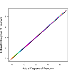
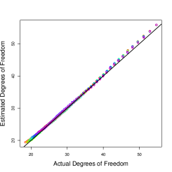
Figure 4: The estimated degrees of freedom as a function of the actual degrees of freedom, for (Left:) FAMILY.l2  and (Right:) FAMILY.linf. To estimate the degrees of freedom for FAMILY.linf, we used $q=500$ in (30). Several values of $\alpha$ in were used in the FAMILY optimization problem (using the reparametrization in (33)); each is shown in a different color. Each point corresponds to a different value of $\lambda$ in the FAMILY optimization problem.

4 Extension to Weak Heredity

We now consider a modification to the FAMILY optimization problem, (6), that imposes weak heredity. We assume that the main effects, interactions, and response have been centered to have mean zero.

In order to enforce weak heredity, we take an approach motivated by the latent overlap group lasso of Jacob et al. (2009). We let $W^{X}$ denote the $n\times p_{1}\times(p_{2}+1)$ array defined as follows: for $i\in\{1,\ldots,n\},\ j\in\{1,\ldots,p_{1}\},\ k\in\{0,\ldots,p_{2}\},$

$$W^{X}_{i,j,k}=\begin{cases}X_{i,j}Z_{i,k}&\mbox{ for }k\not=0\\ X_{i,j}&\mbox{ for }k=0\\ \end{cases}.$$ (31)

We let $W^{Z}$ denote the $n\times(p_{1}+1)\times p_{2}$ array defined in an analogous way. We take $B^{X}$ to be a $p_{1}\times(p_{2}+1)$ matrix, and $B^{Z}$ to be a $(p_{1}+1)\times p_{2}$ matrix.

We propose to solve the optimization problem

$$\begin{split}\underset{\parbox{101.17755pt}{ $B^{X}\in\mathbb{R}^{p_{1}\times(p_{2}+1)}\\ B^{Z}\in\mathbb{R}^{(p_{1}+1)\times p_{2}}$ }}{\text{minimize}}\ &\frac{1}{2n}\left\|y-W^{X}*B^{X}-W^{Z}*B^{Z}\right\|_{2}^{2}\\ &+\lambda_{1}\sum_{j=1}^{p_{1}}P_{r}(B^{X}_{j,.})+\lambda_{2}\sum_{k=1}^{p_{2}}P_{c}(B^{Z}_{.,k})+\lambda_{3}(\|B^{X}_{.,-0}\|_{1}+\|B^{Z}_{-0,.}\|_{1}).\end{split}$$ (32)

Then the coefficient for the $j^{th}$ main effect of $X$ is ${B}^{X}_{j,0}$, the coefficient for the $k^{th}$ main effect of $Z$ is ${B}^{Z}_{0,k}$, and the coefficient for the $(j,k)$ interaction is ${B}^{X}_{j,k}+{B}^{Z}_{j,k}$. If we take $P_{r}$ and $P_{c}$ to be either $\ell_{2}$, $\ell_{\infty}$, or hybrid $\ell_{1}$/$\ell_{\infty}$ penalties, then (32) imposes weak heredity: if the $k$th column of $B_{Z}$ has a zero estimate, then the $(j,k)^{th}$ interaction coefficient estimate need not be zero. However, if the $j^{th}$ row of $B_{X}$ and the $k^{th}$ column of $B_{Z}$ have zero estimates, then the $(j,k)^{th}$ interaction coefficient estimate is zero.

Problem (32) can be solved using an ADMM algorithm similar to that of Section 2.3. Since the focus of this paper is on enforcing strong heredity, we leave the details of an algorithm for (32), as well as a careful numerical study, to future work.

5 Simulation Study

We compare the performance of FAMILY.l2 and FAMILY.linf to the all-pairs lasso (APL), the hierNet proposal of Bien et al. (2013), and the glinternet proposal of Lim and Hastie (2013). APL can be performed using the glmnet R package, and hierNet and glinternet are implemented in R packages available on CRAN. We also include the oracle model (Fan and Li, 2001) — an unpenalized model that uses only the main effects and interactions that are non-zero in the true model — in our comparisons.

The forward selection proposal of Hao and Zhang (2014), iFORM, is a fast screening approach for detecting interactions in ultra-high dimensional data. iFORM is intended for the setting in which the true model is extremely sparse. In our simulation setting, we consider moderately sparse models, which fails to highlight the advantages of iFORM. Thus, we do not include results for iFORM in our simulation study.

To facilitate comparison with hierNet and glinternet, which require $X=Z$, we take $X=Z$ in our simulation study. Similar empirical results are obtained in simulations with $X\neq Z$; results are omitted due to space constraints.

We consider squared error loss in Section 5.1, and logistic regression loss in Section 5.2.

5.1 Squared Error Loss

5.1.1 Simulation Set-up

We created a coefficient matrix $B$, with $p=30$ main effects and ${p\choose 2}=435$ interactions, for a total of $465$ features. The first 10 main effects have non-zero coefficients, assigned uniformly from the set $\{-5,-4,\ldots,-1,1,\ldots,5\}$. The remaining main effects’ coefficients equal zero. We consider three simulation settings, in which we randomly select 15, 30 or 45 non-zero interaction coefficients, chosen to obey strong heredity. The values for the non-zero coefficients were selected uniformly from the set $\{-10,-8,\ldots,-2,2,\ldots,8,10\}$. Figure 5 displays $B$ in each of the three simulation settings.

We generated a training set, a test set, and a validation set, each consisting of 300 observations. Each observation of $X=Z$ was generated independently from a $\mathcal{N}_{p}(0,I)$ distribution; $W$ was then constructed according to (2). For each observation we generated an independent Gaussian noise term, with variance adjusted to maintain a signal-to-noise ratio of approximately 2.5 to 3.5. Finally, for each observation, a response was generated according to (3).

We applied glinternet and hierNet for 50 different values of the tuning parameters. For convenience, given that $X=Z$, we reparametrized the FAMILY optimization problem (6) as

$$\begin{split}\underset{B\in\mathbb{R}^{(p+1)\times(p+1)}}{\text{minimize}}\ \frac{1}{2n}\|y-W*B\|_{2}^{2}&+(1-\alpha)\lambda\sqrt{p}\sum_{j=1}^{p}P_{r}(B_{j,.})+(1-\alpha)\lambda\sqrt{p}\sum_{k=1}^{p}P_{c}(B_{.,k})\\ &+\alpha\lambda\|B_{-0,-0}\|_{1}.\end{split}$$ (33)

We applied FAMILY.l2 and FAMILY.linf over a $10\times 50$ grid of $(\alpha,\lambda)$ values, with $\alpha\in(0,1)$ and $\lambda$ chosen to give a suitable range of sparsity.

Figure 5: For the simulation study in Section 5, the heatmap of the matrix $B$ is displayed in the case of 15 (left), 30 (center), and 45 (right) non-zero interactions. The first row and column of each heatmap represent the main effects.

In principle, many methods are available for selecting the tuning parameters $\alpha$ and $\lambda$. These include Bayesian information criterion, generalized cross-validation, and others. Because we do not have an estimator for the degrees of freedom of the glinternet estimator, we opted to use a training/test/validation set approach. In greater detail, we fit each method to the training set, selected tuning parameters based on sum of squared residuals (SSR) on the test set, and then reported the SSR for that choice of tuning parameters on the validation set.

It is well-known that penalized regression techniques tend to yield models with over-shrunken coefficient estimates (Hastie et al., 2009; Fan and Li, 2001). To overcome this problem, we obtained relaxed versions of FAMILY.l2, FAMILY.linf, hierNet, and glinternet, by refitting an unpenalized least squares model to the set of coefficients that are non-zero in the penalized fitted model (Meinshausen, 2007; Radchenko and James, 2010).

We also considered generating the observations of $X$ from a $\mathcal{N}_{p}(0,\Sigma)$ distribution, where $\Sigma$ was an autoregressive or an exchangeable covariance matrix. We found that the choice of covariance matrix $\Sigma$ led to little qualitative difference in the results. Therefore, we display only results for $\Sigma=I$ in Section 5.1.2.

5.1.2 Results

The left panel of Figure 6 displays ROC curves for FAMILY.linf, FAMILY.l2, hierNet, glinternet, and APL. These results indicate that FAMILY.l2 outperforms all other methods in terms of variable selection, especially as the number of non-zero interaction coefficients increases. When there are 45 non-zero interactions, FAMILY.linf outperforms glinternet, hierNet, and APL.

The right panel of Figure 6 displays the test set SSR for all methods, as the tuning parameters are varied. We observe that relaxation leads to improvement for each method: it yields a much sparser model for a given value of the test error. This is not surprising, since the relaxation alleviates some of the over-shrinkage induced by the application of multiple convex penalties. The results further indicate that when relaxation is applied, FAMILY.l2 performs the best, followed by FAMILY.linf and then the other competitors. We once again observe that the improvement of FAMILY.l2 and FAMILY.linf over the competitors increases as the number of non-zero interaction coefficients increases.

Interestingly, the right-hand panel of Figure 6 indicates that though FAMILY.l2 performs the best when relaxation is performed, it performs quite poorly when relaxation is not performed, in that the model with smallest test set SSR contains far too many non-zero interactions. This is consistent with the remark in Radchenko and James (2010) regarding over-shrinkage of coefficient estimates.

In Table 1, we present results on the validation set for the model that was fit on the training set using the tuning parameters selected on the test set, as described in Section 5.1.1. We see that FAMILY.l2 and FAMILY.linf outperform the competitors in terms of SSR, false discovery rate, and true positive rate, especially when relaxation is performed.

15 Non-Zero Interactions

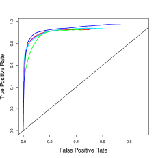
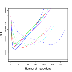
30 Non-Zero Interactions

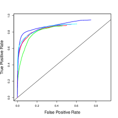
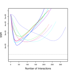
45 Non-Zero Interactions

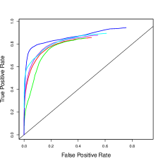
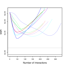
Figure 6: Results for the simulation study of Section 5.1, averaged over 100 simulated datasets. The colored lines indicate the results for glinternet (), hierNet (), APL (), FAMILY.l2 with $\alpha=0.7$ (), and FAMILY.linf with $\alpha=0.83$ (). Left: ROC curves for each proposal, along with the $45^{\circ}$ line. Right: Sum of squared residuals (SSR), evaluated on the test set. Each method is shown with () and without () relaxation. The two horizontal black lines indicate the test set SSR of the true model () and of the oracle model ().

	Method	Relaxed	Relative SSR	FDR	TPR	Num. Inter.
15	FAMILY.l2	No	1.333 (0.012)	0.892 (0.002)	0.931 (0.006)	132.01 (2.3)
		Yes	1.133 (0.010)	0.399 (0.017)	0.837 (0.009)	22.94 (0.8)
	FAMILY.linf	No	1.348 (0.011)	0.855 (0.003)	0.915 (0.006)	97.85 (1.7)
		Yes	1.179 (0.011)	0.304 (0.017)	0.771 (0.010)	17.87 (0.6)
	glinternet	No	1.288 (0.011)	0.786 (0.004)	0.889 (0.007)	64.85 (1.4)
		Yes	1.230 (0.010)	0.209 (0.017)	0.691 (0.011)	14.23 (0.6)
	hierNet	No	1.359 (0.012)	0.816 (0.003)	0.881 (0.007)	73.12 (1.2)
		Yes	1.355 (0.013)	0.382 (0.023)	0.632 (0.013)	19.76 (1.4)
	APL	No	1.341 (0.011)	0.816 (0.004)	0.895 (0.007)	75.90 (1.6)
		Yes	1.308 (0.012)	0.375 (0.019)	0.749 (0.011)	20.65 (1.0)
30	FAMILY.l2	No	1.492 (0.016)	0.841 (0.003)	0.884 (0.006)	172.00 (3.3)
		Yes	1.218 (0.012)	0.352 (0.014)	0.800 (0.010)	39.09 (1.1)
	FAMILY.linf	No	1.476 (0.016)	0.790 (0.004)	0.846 (0.007)	124.00 (2.2)
		Yes	1.276 (0.013)	0.310 (0.016)	0.735 (0.008)	34.11 (1.0)
	glinternet	No	1.487 (0.015)	0.730 (0.005)	0.800 (0.007)	91.75 (1.8)
		Yes	1.446 (0.016)	0.328 (0.017)	0.627 (0.010)	31.07 (1.3)
	hierNet	No	1.567 (0.016)	0.754 (0.003)	0.797 (0.008)	98.95 (1.7)
		Yes	1.677 (0.019)	0.581 (0.013)	0.647 (0.012)	50.90 (1.8)
	APL	No	1.492 (0.016)	0.751 (0.004)	0.821 (0.007)	101.73 (1.8)
		Yes	1.484 (0.018)	0.411 (0.016)	0.676 (0.010)	37.78 (1.4)
45	FAMILY.l2	No	1.562 (0.020)	0.816 (0.003)	0.889 (0.005)	223.29 (4.0)
		Yes	1.219 (0.016)	0.203 (0.016)	0.833 (0.008)	49.09 (1.2)
	FAMILY.linf	No	1.531 (0.019)	0.754 (0.003)	0.841 (0.006)	156.59 (2.6)
		Yes	1.324 (0.023)	0.200 (0.019)	0.756 (0.009)	45.78 (1.5)
	glinternet	No	1.658 (0.021)	0.679 (0.004)	0.776 (0.005)	110.28 (1.4)
		Yes	1.689 (0.025)	0.415 (0.012)	0.610 (0.009)	50.07 (1.7)
	hierNet	No	1.746 (0.023)	0.699 (0.003)	0.772 (0.006)	116.46 (1.5)
		Yes	1.876 (0.027)	0.585 (0.006)	0.650 (0.008)	72.29 (1.5)
	APL	No	1.616 (0.021)	0.693 (0.004)	0.802 (0.005)	119.73 (1.8)
		Yes	1.633 (0.023)	0.456 (0.012)	0.674 (0.008)	59.40 (1.8)

Table 1: Simulation results, averaged over 100 simulated datasets, for the simulation set-up in Section 5.1. Tuning parameters were selected using a training/test/validation set approach, as described in Section 5.1.1. From left to right, the table’s columns indicate the true number of non-zero interactions, the method used, whether or not relaxation was performed, the sum of squared residuals (SSR) on the validation set divided by the SSR of the oracle, the false discovery rate for the detection of non-zero interactions, the true positive rate for the detection of non-zero interactions, and the number of estimated non-zero interactions. Standard errors of the mean are reported in parentheses.

5.2 Logistic regression

5.2.1 Simulation Set-up

We assume that each response $y_{i}$ is a Bernoulli variable with probability $p_{i}$. We then model $p_{i}$ as

$$\log\left(\frac{p_{i}}{1-p_{i}}\right)=(W*B)_{i};\ i=1,\ldots,n,$$ (34)

where $W*B$ is the $n$-vector defined in Section 1.1. The matrices $X$ and $B$ are generated in the exact same manner as in Section 5.1.1, but now with $n=500$ observations in the training and test sets.

Once again, for convenience, we reparametrized FAMILY.l2 and FAMILY.linf according to

$$\begin{split}\underset{B\in\mathbb{R}^{(p+1)\times(p+1)}}{\text{minimize}}&-\frac{1}{n}\sum_{i=1}^{n}\left[y_{i}(W*B)_{i}-\log\left(1+e^{(W*B)_{i}}\right)\right]\\ &+\sqrt{p}(1-\alpha)\lambda\sum_{j=1}^{p}P_{r}(B_{j,.})+\sqrt{p}(1-\alpha)\lambda\sum_{k=1}^{p}P_{c}(B_{.,k})+\alpha\lambda\|B_{-0,-0}\|_{1}.\end{split}$$ (35)

5.2.2 Results

The results for logistic regression are displayed in Figure 7. The ROC curves in the left-hand panel indicate that FAMILY.linf and FAMILY.l2 outperform the competitors in terms of variable selection when there are 30 or 45 non-zero interactions. The SSR curves in the right-hand panel of Figure 7 indicate that the relaxed versions of FAMILY.linf and FAMILY.l2 perform very well in terms of prediction error on the test set, especially as the number of non-zero interactions increases.

15 Non-Zero Interactions

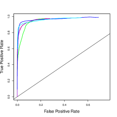
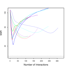
30 Non-Zero Interactions

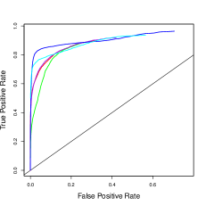
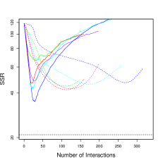
45 Non-Zero Interactions

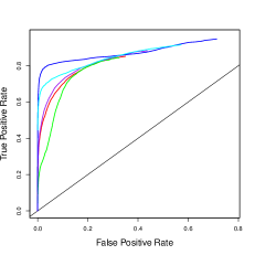
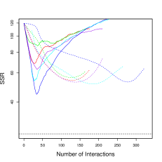
Figure 7: Results for the simulation study of Section 5.2, averaged over 100 simulated data sets. Details are as in Figure 6, but with $\alpha=0.8$ for FAMILY.linf ().

6 Application to HIV Data

Rhee et al. (2006) study the susceptibility of the HIV-1 virus to 6 nucleoside reverse transcriptase inhibitors (NRTIs). The HIV-1 virus can become resistant to drugs via mutations in its genome sequence. Therefore, there is a need to model HIV-1’s drug susceptibility as a function of mutation status. We consider one particular NRTI, 3TC. The data consists of a sparse binary matrix, with mutation status at each of $217$ genomic locations for $n=1057$ HIV-1 isolates. For each of the observations, there is a measure of susceptibility to 3TC. This data set was also studied by Bien et al. (2013).

Rather than working with all $217$ genomic locations, we create bins of ten adjacent loci; this results in a design matrix with $p=22$ features and $n=1057$ observations. We perform the binning because the raw data contains mostly zeros, as most mutations occur in at most a few of the observations; by binning the observations, we obtain less sparse data. This binning is justified under the assumption that mutations in a particular region of the genome sequence result in a change to a binding site, in which case nearby mutations should have similar effects on a binding site, and hence similar associations with drug susceptibility. This binning is also needed for computational reasons, in order to allow for comparison to hierNet (specifically the version that enforces strong heredity) using the R package of Bien et al. (2013). (In Bien et al. (2013), all $217$ genomic locations are analyzed using a much faster algorithm that enforces weak (rather than strong) heredity.)

We split the observations into equally-sized training and test sets. We fit glinternet, hierNet, FAMILY.l2, and FAMILY.linf on the training set for a range of tuning parameter values, and applied the fitted models to the test set. In Figure 8, the test set SSR is displayed as a function of the number of non-zero estimated interaction coefficients, averaged over 50 splits of the data into training and test sets. The figure reveals that all four methods give roughly similar results.

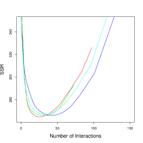
Figure 8: The test set SSR is displayed for the HIV-1 data of Section 6, as a function of the number of non-zero interaction terms. Results are averaged over 50 splits of the observations into a training set and a test set. The colored lines indicate the results for glinternet () , hierNet (), FAMILY.l2 with $\alpha=0.944$ (), and FAMILY.linf with $\alpha=0.944$ ().

Figure 9 displays the estimated coefficient matrix, $\hat{B}$, that results from applying each of the four methods to all $n=1057$ observations using the tuning parameter values that minimized the average test set SSR. The estimated coefficients are qualitatively similar for all four methods. All four methods detect some non-zero interactions involving the 17th feature. Glinternet yields the sparsest model.

(a)                                                      (b)

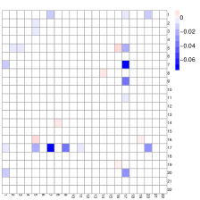
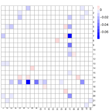
(c)                                                      (d)

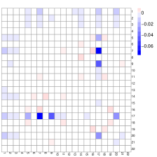
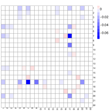
Figure 9: For the HIV-1 data of Section 6, the estimated coefficient matrix $\hat{B}_{-0,-0}$ is shown for (a): glinternet; (b): hierNet; (c): FAMILY.l2 with $\alpha=0.944$; and (d): FAMILY.linf with $\alpha=0.944$. Main effects are not displayed.

7 Conclusion

In this paper, we have introduced FAMILY, a framework that unifies a number of existing estimators for high-dimensional models with interactions. Special cases of FAMILY correspond to the all-pairs lasso, the main effects lasso, VANISH, and hierNet. Furthermore, we have explored the use of FAMILY with $\ell_{2}$, $\ell_{\infty}$, and hybrid $\ell_{1}$/$\ell_{\infty}$ penalties; these result in strong heredity and have good empirical performance.

The empirical results in Sections 5 and 6 indicate that the choice of penalty in FAMILY may be of little practical importance: for instance, FAMILY.l2, FAMILY.linf, and FAMILY.hierNet have similar performance. However, one could choose among penalties using cross-validation or a related approach.

We have presented a simple ADMM algorithm that can be used to solve the FAMILY optimization problem for any convex penalty. It finds the global optimum for VANISH (unlike the proposal in Radchenko and James (2010)), and provides a simpler alternative to the original hierNet algorithm (Bien et al., 2013).

FAMILY could be easily extended to accommodate higher-order interaction models. For instance, to accommodate third-order interactions, we could take $B$ to be a $(p+1)\times(p+1)\times(p+1)$ coefficient array. Instead of penalizing each row and each column of $B$, we would instead penalize each ‘slice’ of the array.

In the simulation study in Section 5, we considered a setting with only $p_{1}=p_{2}=30$ main effects. We did this in order to facilitate comparison to the hierNet proposal, which is very computationally intensive as implemented in the R package of Bien et al. (2013). However, our proposal can be applied for much larger values of $p_{1}$ and $p_{2}$, as discussed in Section 2.3.3.

The R package FAMILY, available on CRAN, implements the methods described in this paper.

Appendix A Alternating Directions Method of Multipliers

A.1 Overview of ADMM

We will solve (6) using the alternating directions method of multipliers (ADMM) algorithm, which we briefly review here. We refer the reader to Boyd et al. [2011] for a detailed discussion.

ADMM provides a simple, general, and efficient approach for solving a problem of the form

$$\underset{x}{\text{minimize }}f_{1}(x)+f_{2}(x),$$ (A.1)

where $f_{1}$ and $f_{2}$ are convex, closed and proper. The key insight behind ADMM is that (A.1) can be re-written as

$$\underset{x,y}{\text{minimize }}\{f_{1}(x)+f_{2}(y)\}\mbox{ subject to }x=y.$$ (A.2)

The augmented Lagrangian corresponding to (A.2) takes the form

$$L_{\rho}(x,y,\gamma)=f_{1}(x)+f_{2}(y)+\gamma(x-y)+(\rho/2)\|x-y\|_{2}^{2},$$

where $\gamma$ is a dual variable and $\rho\in\mathbb{R}$ is a positive constant. The resulting ADMM algorithm involves iterating the following steps until convergence,

$$x^{k+1} =\underset{x}{\text{argmin }}L_{\rho}(x,y^{k},\gamma^{k})$$

$$y^{k+1} =\underset{y}{\text{argmin }}L_{\rho}(x^{k+1},y,\gamma^{k})$$

$$\gamma^{k+1} =\gamma^{k}+\rho(x^{k+1}-y^{k+1})\ ,$$

where $k$ indexes the iterations. Under a few simple conditions, the ADMM algorithm converges to the global optimum [Boyd et al., 2011].

A.2 FAMILY with Squared Error Loss

A.2.1 The ADMM Algorithm

The augmented Lagrangian corresponding to (6) was given in (16). The complete ADMM algorithm is as follows:

1. Initialize ${\rho^{0},\ B^{0},\ \Theta^{0}\text{ and }\Gamma^{0}}$.

2. Choose $\varepsilon^{pri}>0$, $\varepsilon^{dual}>0$.

3. Repeat for $i=1,2,3,...$ until $r^{i}<\varepsilon^{pri}$ and $s^{i}<\varepsilon^{dual}$, where $r^{i}$ and $s^{i}$ are the primal and dual residuals, respectively, defined as

   $$s^{i} =\rho^{i}\|(D^{i}|E^{i}|F^{i})-(D^{i-1}|E^{i-1}|F^{i-1})\|_{F}$$

   $$r^{i} =\|(B^{i}|B^{i}|B^{i})-(D^{i}|E^{i}|F^{i})\|_{F}.$$

   1. Update $\rho^{i}$ as described in Boyd et al. [2011]:

      $$\rho^{i}=\left\{\begin{array}[]{cc}2\rho^{i-1}&\mbox{if}\;\;r^{i-1}>10s^{i-1}\\ \rho^{i-1}/2&\mbox{if}\;\;10r^{i-1}<s^{i-1}\\ \rho^{i-1}&\text{ otherwise }\end{array}\right..$$

   2. Update ${B^{i}}$ as the solution to the least squares problem:

      $$\begin{split}B^{i}=\ &\underset{B}{\text{argmin}}\ \ \frac{1}{2n}\|{y}-{W}*B\|_{2}^{2}\\ &+\frac{3\rho^{i}}{2}\left\|\frac{1}{3\rho^{i}}\left[\rho^{i}(D^{i-1}+E^{i-1}+F^{i-1})-(\Gamma_{1}^{i-1}+\Gamma_{2}^{i-1}+\Gamma_{3}^{i-1})\right]-B\right\|_{F}^{2}.\end{split}$$

   3. Update ${D^{i}}$ and $E^{i}$ using the proximal operators discussed in Section 2.3.2:

      $$D^{i} =\underset{D}{\text{argmin}}\ \ \frac{\rho^{i}}{2}\left\|{D}-\left({B^{i}}+\frac{{\Gamma_{1}^{i-1}}}{\rho^{i}}\right)\right\|_{F}^{2}+\lambda_{1}\sum_{j=1}^{p_{1}}P_{r}({D}_{j,.}),$$

      $$E^{i} =\underset{E}{\text{argmin}}\ \ \frac{\rho^{i}}{2}\left\|{E}-\left({B^{i}}+\frac{{\Gamma^{i-1}_{2}}}{\rho^{i}}\right)\right\|_{F}^{2}+\lambda_{2}\sum_{j=1}^{p_{2}}P_{c}({E}_{.,k})$$

   4. Update $F^{i}$ as follows:

      $${F}^{i}_{0,.} ={B}^{i}_{0,.}+\frac{{\Gamma_{3}}^{i-1}_{0,.}}{{\rho^{i}}},$$

      $${F}^{i}_{.,0} ={B}^{i}_{.,0}+\frac{{\Gamma_{3}}^{i-1}_{.,0}}{\rho^{i}},$$

      $${F}^{i}_{j,k} =\text{sign}\left({B}^{i}_{j,k}+\frac{{\Gamma_{3}}^{i-1}_{j,k}}{{\rho^{i}}}\right)\left(\left|{B}^{i}_{j,k}+\frac{{\Gamma_{3}}^{i}_{j,k}}{{\rho^{i}}}\right|-\frac{\lambda_{3}}{\rho^{i}}\right)_{+}\ \ \text{ for }j\not=0,k\not=0.$$

   5. Update ${\Gamma}^{i}$ as follows:

      $${\Gamma}_{1}^{i} ={\Gamma_{1}}^{i-1}+\rho^{i}\left({B}^{i}-{D}^{i}\right),$$

      $${\Gamma}_{2}^{i} ={\Gamma_{2}}^{i-1}+\rho^{i}\left({B}^{i}-{E}^{i}\right),$$

      $${\Gamma}_{3}^{i} ={\Gamma_{3}}^{i-1}+\rho^{i}\left({B}^{i}-{F}^{i}\right).$$

A.2.2 Update for $B$ in Step 3(b)

The update for $B$ in Step 3(b) is a least squares problem with a $n\times(p_{1}+1)(p_{2}+1)$ design matrix. Here we show that clever matrix algebra can be applied in order to avoid solving this least squares problem in each iteration. For convenience, we omit the superscripts in Step 3(b).

Let $\widetilde{B},\widetilde{D},\widetilde{E},\widetilde{F},\widetilde{\Gamma}_{1},\widetilde{\Gamma}_{2}$, and $\widetilde{\Gamma}_{3}$ denote the vectorized versions of ${B},{D},{E},{F},{\Gamma}_{1},{\Gamma}_{2}$, and ${\Gamma}_{3}$. And let $\widetilde{W}$ denote the $n\times(p_{1}+1)(p_{2}+1)$-dimensional matrix version of $W$. Then the objective of Step 3(b) can be rewritten as

$$\frac{1}{2}\left\|\left[\begin{array}[]{c}\frac{1}{\sqrt{n}}{y}\\ \frac{\rho{(\widetilde{D}+\widetilde{E}+\widetilde{F})}-({\widetilde{\Gamma}_{1}+\widetilde{\Gamma}_{2}+\widetilde{\Gamma}_{3}})}{\sqrt{3\rho}}\\ \end{array}\right]-\left[\begin{array}[]{c}\frac{1}{\sqrt{n}}\widetilde{W}\\ \sqrt{3\rho}{I}_{(1+p_{1})(1+p_{2})}\\ \end{array}\right]\widetilde{B}\right\|_{F}^{2}.$$ (A.3)

Therefore, before performing the ADMM algorithm described in Section A.2, we compute the SVD of $\widetilde{W}$. Then for each iteration of Step 3(b), the Woodbury matrix identity can be very quickly applied in order to minimize (A.3).

A.3 FAMILY for Generalized Linear Models

We now consider the extension of FAMILY to GLMs (Section 2.4). The resulting ADMM algorithm is as in Section A.2, except that the update for $B$ in Step 3(b) now takes the form

$$\footnotesize\underset{B\in\mathbb{R}^{(p_{1}+1)\times(p_{2}+1)}}{\text{argmin }}\ \ \frac{1}{n}l(WB)+\frac{3\rho^{i}}{2}\left\|\frac{1}{3\rho^{i}}\left[\rho^{i}(D^{i-1}+E^{i-1}+F^{i-1})-(\Gamma_{1}^{i-1}+\Gamma_{2}^{i-1}+\Gamma_{3}^{i-1})\right]-B\right\|_{F}^{2}.$$ (A.4)

To solve this problem, we perform a second-order Taylor expansion of (A.4), in which we approximate the Hessian using a multiple of the identity (e.g., for logistic regression, we use the upper bound of $(1/4)I$). Details are omitted in the interest of brevity.

Appendix B Proofs of Results in Section 2

Proof of Lemma 2.2.

The result follows from the definition of the dual norm.

$$P_{*}(z) =\sup\{z^{T}\beta:P(\beta)\leq 1\}$$

$$=\sup\{z^{T}\beta:\max(|\beta_{1}|,\|\beta_{-1}\|_{1})\leq 1\}$$

$$=\sup\{z^{T}\beta:|\beta_{1}|\leq 1\text{ and }\|\beta_{-1}\|_{1}\leq 1\}$$

$$=\sup\{z_{1}\beta_{1}+z_{-1}^{T}\beta_{-1}:|\beta_{1}|\leq 1\text{ and }\|\beta_{-1}\|_{1}\leq 1\}$$

$$=\sup\{z_{1}\beta_{1}:|\beta_{1}|\leq 1\}+\sup\{z_{-1}^{T}\beta_{-1}:\|\beta_{-1}\|_{1}\leq 1\}$$

$$=|z_{1}|+\|z_{-1}\|_{\infty}.$$

∎

Proof of Lemma 2.3.

Consider the series of equalities:

$$\min_{\beta}\ \frac{1}{2}\|y-\beta\|^{2}+\lambda P(\beta) =\min_{\beta}\max_{P_{*}(u)\leq\lambda}\ \frac{1}{2}\|y-\beta\|^{2}+\beta^{T}u$$

$$=\max_{P_{*}(u)\leq\lambda}\min_{\beta}\frac{1}{2}\|y-\beta\|^{2}+\beta^{T}u$$

$$=\max_{P_{*}(u)\leq\lambda}\frac{1}{2}\|y-(y-u)\|^{2}+(y-u)^{T}u$$

$$=\max_{P_{*}(u)\leq\lambda}y^{T}u-\frac{1}{2}\|u\|^{2}$$

$$=\max_{P_{*}(u)\leq\lambda}-\frac{1}{2}\|u-y\|^{2}+constant.$$

This is equivalent to the problem

$$\underset{u\in\mathbb{R}^{p}}{\text{minimize}}\ \frac{1}{2}\|y-u\|^{2}$$

$$\text{subject to }\ |u_{1}|+\|u_{-1}\|_{\infty}\leq\lambda,$$

which, in turn, is equivalent to (17). ∎

B.1 Proof of Theorem 2.4

We consider the function

$$f(\lambda_{1})=\frac{1}{2}\|u(\lambda_{1})-y\|^{2},$$ (B.1)

where $u(\lambda_{1})$ is a vector-valued function of $\lambda_{1}$, as defined in (18). We wish to minimize this function over the interval $[0,\lambda]$. We will prove this theorem using a series of claims.

Claim B.1.

The function $f(\lambda_{1})$ is convex on $\mathbb{R}$.

Proof.

Note that

$$(y_{1}-u_{1}(\lambda_{1}))^{2} =(y_{1}-y_{1})^{2}\boldsymbol{1}(|y_{1}|\leq\lambda_{1})+(y_{1}-\lambda_{1}\mbox{sign}(y_{1}))^{2}\boldsymbol{1}(|y_{1}|>\lambda_{1})$$

$$=(y_{1}-\lambda_{1}\mbox{sign}(y_{1}))^{2}\boldsymbol{1}(|y_{1}|>\lambda_{1})$$ (B.2)

and

$$(y_{i}-u_{i}(\lambda_{1}))^{2} =(y_{i}-(\lambda-\lambda_{1})\mbox{sign}(y_{i}))^{2}\boldsymbol{1}(\lambda_{1}>\lambda-|y_{i}|).$$ (B.3)

By inspection, both (B.2) and (B.3) are convex. The result follows from the fact that the sum of convex functions is convex. ∎

Claim B.2.

The derivative of $f(\lambda_{1})$ is given by

$$\frac{d}{d\lambda_{1}}f(\lambda_{1}) =[\lambda_{1}-|y_{1}|]\boldsymbol{1}(|y_{1}|>\lambda_{1})+\sum_{i=1}^{p-1}\left[\lambda_{1}-z_{(i)}\right]\boldsymbol{1}(\lambda_{1}>z_{(i)}),$$ (B.4)

where $z$ is as defined in Theorem 2.4.

Proof.

Note that $f(\lambda_{1})$ can be rewritten as

$$f(\lambda_{1})=(y_{1}-\lambda_{1}\mbox{sign}(y_{1}))^{2}\boldsymbol{1}(|y_{1}|>\lambda_{1})+\sum_{i=2}^{p}(y_{i}-(\lambda-\lambda_{1})\mbox{sign}(y_{i}))^{2}\boldsymbol{1}(\lambda_{1}>\lambda-|y_{i}|).$$

The result follows by inspection.

∎

Claim B.3.

Define

$$\lambda_{1}(m)=\frac{|y_{1}|+\sum_{j=1}^{m}z_{(j)}}{m+1}.$$ (B.5)

Then

$$\underset{\lambda_{1}\in\mathbb{R}}{\text{argmin}}\ f(\lambda_{1})=\min_{m}\lambda_{1}(m).$$ (B.6)

Proof.

Let $z_{(p)}\equiv\infty$, and define $\lambda_{1}(m)\equiv\frac{|y_{1}|+\sum_{j=1}^{m}z_{(j)}}{m+1}$. The optimality conditions for $f(\lambda_{1})$ guarantee that if $\lambda_{1}(m)\in(z_{(m)},z_{(m+1)}]$, then $\hat{\lambda}_{1}=\lambda_{1}(m)$.

If the set $\arg\min_{m}\lambda_{1}(m)$ contains a single element, then define $k\equiv\arg\min_{m}\lambda_{1}(m)$; otherwise, let $k$ be the smallest element of the set. To complete the proof, it suffices to show that $\lambda_{1}(k)\in(z_{(k)},z_{(k+1)}]$.

First, we will show that $\lambda_{1}(k)>z_{(k)}$. By definition of $\lambda_{1}(k)$, we know that $\lambda_{1}(k)<\lambda_{1}(k-1)$. In other words,

$$\frac{|y_{1}|+\sum_{j=1}^{k}z_{(j)}}{k+1}<\frac{|y_{1}|+\sum_{j=1}^{k-1}z_{(j)}}{k}.$$

Rearranging terms, we find that

$$\left({|y_{1}|+\sum_{j=1}^{k}z_{(j)}}\right)\left(1-\frac{1}{k+1}\right)<{|y_{1}|+\sum_{j=1}^{k-1}z_{(j)}}.$$

Consequently,

$$z_{(k)}-\frac{|y_{1}|+\sum_{j=1}^{k}z_{(j)}}{k+1}<0.$$

This means that $z_{(k)}<\lambda_{1}(k)$.

We now use a similar argument to show that $\lambda_{1}(k)\leq z_{(k+1)}$. By definition of $\lambda_{1}(k)$, we know that $\lambda_{1}(k)\leq\lambda_{1}(k+1)$. In other words,

$$\frac{|y_{1}|+\sum_{j=1}^{k}z_{(j)}}{k+1}\leq\frac{|y_{1}|+\sum_{j=1}^{k+1}z_{(j)}}{k+2}.$$

Rearranging terms, we find that

$$\left({|y_{1}|+\sum_{j=1}^{k}z_{(j)}}\right)\left(1+\frac{1}{k+1}\right)\leq{|y_{1}|+\sum_{j=1}^{k+1}z_{(j)}}=\left(|y_{1}|+\sum_{j=1}^{k}z_{(j)}\right)+z_{(k+1)}.$$

This implies that $\lambda_{1}(k)\leq z_{(k+1)}$. ∎

Since $f(\lambda_{1})$ is convex, its minimizer in the interval $[0,\lambda]$ is simply the projection of its minimizer on $\mathbb{R}$ (given in Claim B.3) into the interval. This completes the proof of Theorem 2.4.

∎

Appendix C Degrees of Freedom for FAMILY

Derivation of Claim 3.2.

As mentioned in the main text, an unbiased estimate for the degrees of freedom of (26) is given by

$$\widehat{\mathrm{df}}=\sum_{i=1}^{n}\frac{\partial\hat{y}_{i}}{\partial y_{i}}=\mathrm{trace}\left(\frac{d\hat{y}}{dy}\right),$$ (C.1)

provided that $\hat{y}(y)$ is almost differentiable. The proof that $\hat{y}(y)$ is almost differentiable follows from arguments similar to those in Tibshirani et al. [2012].

We now derive an explicit form for (C.1). To evaluate $\frac{d\hat{y}}{dy}$, we first note that $\hat{\beta}_{\mathcal{A}}$, the solution of (26) restricted to the active set, takes the form

$$\hat{\beta}_{\mathcal{A}}=\underset{\beta_{\mathcal{A}}}{\text{argmin}}\ \left\{\frac{1}{2}\|y-X_{\mathcal{A}}\beta_{\mathcal{A}}\|_{2}^{2}+\sum_{d}\lambda_{d}P_{d}(A_{d}^{\mathcal{A}}\beta_{\mathcal{A}})\right\}.$$ (C.2)

Therefore, $\hat{\beta}_{\mathcal{A}}$ must satisfy

$$-{X}_{\mathcal{A}}^{T}(y-{X}_{\mathcal{A}}\hat{\beta}_{\mathcal{A}})+\sum_{d}\lambda_{d}(A^{\mathcal{A}}_{d})^{T}\dot{P}_{d}(A^{\mathcal{A}}_{d}\hat{\beta}_{\mathcal{A}})=0.$$ (C.3)

We then differentiate with respect to $y$ and apply the chain rule, to obtain

$$-{X}_{\mathcal{A}}^{T}+{X}_{\mathcal{A}}^{T}{X}_{\mathcal{A}}\frac{d\hat{\beta}_{\mathcal{A}}}{dy}+\sum_{d}\lambda_{d}(A^{\mathcal{A}}_{d})^{T}\ddot{P}_{d}(A^{\mathcal{A}}_{d}\hat{\beta}_{\mathcal{A}})\left(A^{\mathcal{A}}_{d}\right)\frac{d\hat{\beta}_{\mathcal{A}}}{dy}=0.$$ (C.4)

Solving for $\frac{d\hat{\beta}_{\mathcal{A}}}{dy}$ gives us

$$\frac{d\hat{\beta}_{\mathcal{A}}}{dy}=\left[{X}_{\mathcal{A}}^{T}{X}_{\mathcal{A}}+\sum_{d}\lambda_{d}(A^{\mathcal{A}}_{d})^{T}\ddot{P}_{d}(A^{\mathcal{A}}_{d}\hat{\beta}_{\mathcal{A}})(A^{\mathcal{A}}_{d})\right]^{-1}{X}_{\mathcal{A}}^{T}.$$ (C.5)

Form the definition of $\hat{y}=X_{\mathcal{A}}\hat{\beta}_{\mathcal{A}}$, we get

$$\frac{d\hat{y}}{dy}={X}_{\mathcal{A}}\frac{d\hat{\beta}_{\mathcal{A}}}{dy}={X}_{\mathcal{A}}\left[{X}_{\mathcal{A}}^{T}{X}_{\mathcal{A}}+\sum_{d}\lambda_{d}(A^{\mathcal{A}}_{d})^{T}\ddot{P}_{d}(A^{\mathcal{A}}_{d}\hat{\beta}_{\mathcal{A}})(A^{\mathcal{A}}_{d})\right]^{-1}{X}_{\mathcal{A}}^{T}.$$ (C.6)

In order to make this derivation entirely rigorous, we would need to show that $\hat{\beta}$ is unique, and that with probability one, within some neighbourhood of $y$, the active set $\mathcal{A}$ does not change as a function of $y$.

∎

References

- Bach et al. [2011] Francis Bach, Rodolphe Jenatton, Julien Mairal, Guillaume Obozinski, et al. Convex optimization with sparsity-inducing norms. Optimization for Machine Learning, pages 19–53, 2011.
- Bach et al. [2012] Francis Bach, Rodolphe Jenatton, Julien Mairal, Guillaume Obozinski, et al. Structured sparsity through convex optimization. Statistical Science, 27(4):450–468, 2012.
- Bickel et al. [2010] Peter J Bickel, Ya’acov Ritov, Alexandre B Tsybakov, et al. Hierarchical selection of variables in sparse high-dimensional regression. In Borrowing strength: theory powering applications–a Festschrift for Lawrence D. Brown, pages 56–69. Institute of Mathematical Statistics, 2010.
- Bien et al. [2013] Jacob Bien, Jonathan Taylor, and Robert Tibshirani. A lasso for hierarchical interactions. The Annals of Statistics, 41(3):1111–1141, 2013.
- Boyd et al. [2011] Stephen Boyd, Neal Parikh, Eric Chu, Borja Peleato, and Jonathan Eckstein. Distributed optimization and statistical learning via the alternating direction method of multipliers. Foundations and Trends® in Machine Learning, 3(1):1–122, 2011.
- Chipman [1996] Hugh Chipman. Bayesian variable selection with related predictors. Canadian Journal of Statistics, 24(1):17–36, 1996.
- Choi et al. [2010] Nam Hee Choi, William Li, and Ji Zhu. Variable selection with the strong heredity constraint and its oracle property. Journal of the American Statistical Association, 105(489):354–364, 2010.
- Cox [1984] David R Cox. Interaction. International Statistical Review/Revue Internationale de Statistique, pages 1–24, 1984.
- Duchi and Singer [2009] John Duchi and Yoram Singer. Efficient online and batch learning using forward backward splitting. The Journal of Machine Learning Research, 10:2899–2934, 2009.
- Efron [1986] Bradley Efron. How biased is the apparent error rate of a prediction rule? Journal of the American Statistical Association, 81(394):461–470, 1986.
- Fan and Li [2001] Jianqing Fan and Runze Li. Variable selection via nonconcave penalized likelihood and its oracle properties. Journal of the American Statistical Association, 96(456):1348–1360, 2001.
- Friedman et al. [2007] Jerome Friedman, Trevor Hastie, Holger Höfling, Robert Tibshirani, et al. Pathwise coordinate optimization. The Annals of Applied Statistics, 1(2):302–332, 2007.
- Friedman [1991] Jerome H Friedman. Multivariate adaptive regression splines. The annals of statistics, pages 1–67, 1991.
- George and McCulloch [1993] Edward I George and Robert E McCulloch. Variable selection via gibbs sampling. Journal of the American Statistical Association, 88(423):881–889, 1993.
- Hamada and Wu [1992] Michael Hamada and CF Jeff Wu. Analysis of designed experiments with complex aliasing. Journal of Quality Technology, 24(3):130–137, 1992.
- Hao and Zhang [2014] Ning Hao and Hao Helen Zhang. Interaction screening for ultrahigh-dimensional data. Journal of the American Statistical Association, 109(507):1285–1301, 2014.
- Hastie et al. [2009] Trevor Hastie, Robert Tibshirani, Jerome Friedman, T Hastie, J Friedman, and R Tibshirani. The elements of statistical learning, volume 2. Springer, 2009.
- Jacob et al. [2009] Laurent Jacob, Guillaume Obozinski, and Jean-Philippe Vert. Group lasso with overlap and graph lasso. In Proceedings of the 26th Annual International Conference on Machine Learning, pages 433–440. ACM, 2009.
- Jenatton et al. [2011] Rodolphe Jenatton, Jean-Yves Audibert, and Francis Bach. Structured variable selection with sparsity-inducing norms. The Journal of Machine Learning Research, 12:2777–2824, 2011.
- Joseph [2006] V Roshan Joseph. A bayesian approach to the design and analysis of fractionated experiments. Technometrics, 48(2):219–229, 2006.
- Lim and Hastie [2013] Michael Lim and Trevor Hastie. Learning interactions through hierarchical group-lasso regularization. arXiv preprint arXiv:1308.2719, 2013.
- McCullagh [1984] Peter McCullagh. Generalized linear models. European Journal of Operational Research, 16(3):285–292, 1984.
- Meinshausen [2007] Nicolai Meinshausen. Relaxed lasso. Computational Statistics & Data Analysis, 52(1):374–393, 2007.
- Montgomery et al. [2012] Douglas C Montgomery, Elizabeth A Peck, and G Geoffrey Vining. Introduction to linear regression analysis, volume 821. John Wiley & Sons, 2012.
- Park and Hastie [2008] Mee Young Park and Trevor Hastie. Penalized logistic regression for detecting gene interactions. Biostatistics, 9(1):30–50, 2008.
- Peixoto [1987] Julio L Peixoto. Hierarchical variable selection in polynomial regression models. The American Statistician, 41(4):311–313, 1987.