Gene-Mating Dynamic Evolution Theory I:
Fundamental assumptions, exactly solvable models and analytic solutions
Abstract
Fundamental properties of macroscopic gene-mating dynamic evolutionary systems are investigated. A model is studied to describe a large class of systems within population genetics. We focus on a single locus, any number of alleles in a two-gender dioecious population. Our governing equations are time-dependent continuous differential equations labeled by a set of parameters, where each parameter stands for a population percentage carrying certain common genotypes. The full parameter space consists of all allowed parameters of these genotype frequencies. Our equations are uniquely derived from four fundamental assumptions within any population: (1) a closed system; (2) average-and-random mating process (mean-field behavior); (3) Mendelian inheritance; (4) exponential growth and exponential death. Even though our equations are nonlinear with time-evolutionary dynamics, we have obtained an exact analytic time-dependent solution and an exactly solvable model. Our findings are summarized from phenomenological and mathematical viewpoints. From the phenomenological viewpoint, any initial parameter of genotype frequencies of a closed system will eventually approach a stable fixed point. Under time evolution, we show (1) the monotonic behavior of genotype frequencies, (2) any genotype or allele that appears in the population will never become extinct, (3) the Hardy-Weinberg law, and (4) the global stability without chaos in the parameter space. To demonstrate the experimental evidence for our theory, as an example, we show a mapping from the data of blood type genotype frequencies of world ethnic groups to our stable fixed-point solutions. From the mathematical viewpoint, our highly symmetric governing equations result in continuous global stable equilibrium solutions: These solutions altogether consist of a continuous curved manifold as a subspace of the whole parameter space of genotype frequencies. This fixed-point manifold is a global stable attractor known as the Hardy-Weinberg manifold, attracting any initial point in any Euclidean fiber bounded within the genotype frequency space to the fixed point where this fiber is attached. The stable base manifold and its attached fibers form a fiber bundle, which fills in the whole genotype frequency space completely. We can define the genetic distance of two populations as their geodesic distance on the equilibrium manifold. In addition, the modification of our theory under the process of natural selection and mutation is addressed.
pacs:
87.10.-e, 87.23.-n, 83.80.Lz, 05.45.-aI Introduction
Time evolution of population percentages labeled by biological traits or genetic characteristics
in a population
system is a main subject of studies for population genetics and evolutionary
biology (Wright ; Fisher ; Crowbook ; book1 ; book2 ; book3 and references therein).
Their governing laws may involve classical genetics, which can be traced back to Mendel’s seminal work Mendel .
Both the birth rate and death rate of a system will change the
population number. Also the mating mechanism and inheritance laws will determine
the percentage weight of newborn biological traits. There are abundant past researches and advance studying population genetic questions and equations ( Wright ; Fisher ; Crowbook ; book1 ; book2 ; book3 ). For example, Wright and other pioneer researchers Wright favor use of discrete difference equations to label each generation and the reproduction.
However, the difference equation does not manifest the dynamical properties as transparently as the continuous differential equations,
pioneered by Fisher, Crow and Kimura, et al. Fisher ; Crowbook .
In this work, we will formulate a set of exactly solvable nonlinear differential equations with a first-order time derivative to address
population genetic questions.
Out of curiosity, the authors had posed the following questions to ourselves many years ago:111This model presented here is originated from an independent thought of the first author during his undergrad freshman year.
The governing equations and model are derived in 2003.
Substantial work is completed and exact solutions are found in 2006.
The manuscript presented here is a late update of our 2006’s work aiming to contribute to the academic literature.
How should we characterize an ecological or macroscopic biological system consisting
of a large population of many living beings within a mathematical framework?
How can we characterize the time-dependent evolution of genetic diversity and genotype percentage of a population driven by the mating process and population growth?
Is there a mathematical definition of genetic distance between two population groups even within the same species under the biological taxonomy?
For example, can we quantitatively define the mathematical genetic distance of different ethnic groups of Homo sapiens, human beings? What would be the genetic distance of ethnic groups: Taiwanese, Cantonese, Japanese, Jewish, Irish people, etc.? Similarly, can we quantitatively define the relative genetic distances of other animal or plant species (within the same species), such as Darwin’s finches, studied in Charles Darwin’s “On the Origin of Species” origin ?
To our amusement, however,
even without any necessity of deep biological knowledge,
we can independently derive, from scratch, a set of exactly solvable governing equations describing a universal large class of systems addressing the issues of population genetics and evolutionary biology:
Our model contains time-dependent governing equations together with our four fundamental assumptions.
Our theory incorporates exactly solvable models and their mathematical properties describing population genetic systems.
Our theory provides an answer to each of the questions we posed above.
To the best of our knowledge, the analysis closest to ours in the literature is Ref.Nagylaki . In Ref.Nagylaki , some exact solvable models within a gene pool are analyzed, where the monotonic evolutionary behavior is found.
Our model is similar to Ref.Nagylaki ’s model: Ref.Nagylaki ’s studies a single locus for an arbitrary number of alleles with or without distinguishing the sex
(e.g. monoecious or dioecious organisms222See the comparison of
models of one-gender monoecious population, two-gender dioecious population, and multi-gender population in gene2 , and also in Nagylaki and Crow (1974) Nagylaki .;
we study a single locus, arbitrary number alleles in a two-gender dioecious population.
Though Ref.Nagylaki reaches results similar to ours, we find several new ingredients:
(1) The stable equilibrium solutions as a manifold.
(2) The parameterization of the equilibrium manifold.
(3) The experimental evidence of the model, such as the blood type of human ethnic groups.
We present the experimental data of phenotype (Oexp,Aexp,Bexp,ABexp)
in Table.1, 3, 4.
We present our corresponding theoretical prediction of genotype (Ot,AAt, Ait,BBt,Bit,ABi) in
Table.2, 5, 6. See Sec.VIII for figures.
(4) The proposal to define the genetic distance of two populations as their geodesic distance on the equilibrium manifold in the genotype frequency space.
(5) The exact analytic solution in terms of a Euclidean fiber bundle.
(6) Our work may be viewed as
a unified framework
combining the exact analytic solutions of Ref.Nagylaki with
the stability analysis of the Hardy-Weinberg law Hardy ; Weinberg , together with a proper parameterization of stable equilibrium manifold.
We believe that our work adds value to the literature.
We will work out our model step by step.
To characterize a population genetic system, the first step is to find a good biological parameter to label the system.
The biological trait can be a genotype or phenotype.
Here we will use the genotype, the genetic makeup of an individual.
The genotype contains a set of choices of possible alleles.
We will focus on a genotype determined by a single locus and an arbitrary number of alleles.
We will use the genotype frequency, the number of individuals with a given genotype normalized by the total number of individuals in the population.
A set of genotype frequencies provides the normalized parameter to label the given population.
Throughout the text, we may also term this genotype frequency concept as “percentage parameter” or simply “parameter” of the given population.
The full parameter space consists of all allowed genotype frequencies of the population.
Under governing principles, the genotype frequency can evolve under the time evolution.
In this work, we start from four fundamental assumptions in Sec.II.
In Sec.III, IV: we derive the dynamical governing equations under time evolution.
We solve the time-dependent exact analytic solution (see Fig.1 for an illustration)
from a set of coupled nonlinear differential equations with first-order time derivatives.
We are able to show global
stability, monotonic evolution, and no chaos for any population system.
We prove that any genotype or allele that ever presents in the population will never become extinct
and also derive the Hardy-Weinberg law Hardy ; Weinberg in Sec.IV.
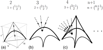
In addition to the analytical work,
we also found experimental data strongly consistent with our study to confirm the validity of our theory.
Specifically, we examine the experimental data
of the
genotype frequency of blood type data for (1) different ethnic groups and (2) different countries, in Sec.III.2. With strong evidence and some expected error bars,
the data can be rigorously fitted into our stable equilibrium solutions of governing equations.
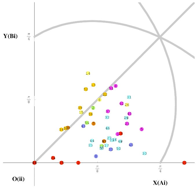
The stable equilibrium manifold can be mapped to a continuous two-dimensional quadrant map. This gives a panorama of how each ethnic group relates to another one. See FIG.2 for an illustration. Our result demonstrates that the laws of inheritance tend to approach stable equilibrium rather than with the usual
chaos or complexity occurring in other nonlinear systems.
In addition to this standard case,
we
further briefly analyze the case incorporating natural selection and mutation.
In Sec. IV.2, we propose that a geodesic distance on the stable fixed-point manifold as a measure of the genetic distance. We comment that the genetic distances have also been studied and proposed in the past in the influential works of cavalli1967phylogenetic nei1972genetic antonelli1977geometry1 , antonelli1977geometry2 , antonelli1977geometry3 , antonelli1978geometry4 , reynolds1983estimation , and see also a recent review dougan2016genetic . However, it is worthwhile to mention that since we have provided an exact analytic stable fixed-point manifold parametrized by Eq.(24) for the general case (Also the Eq.(3) and Eq.(11) for more specific cases), we can precisely solve the geodesic as a continuous path connecting any two points on the stable fixed-point manifold. This has a better advantage to define a continuous measure of genetic distances, while some of the previous work use the discretized measures can only achieve a discretized distance measurement for genetic distances of different populations of the same given species, and cannot obtain a continuous varying distance measurement.
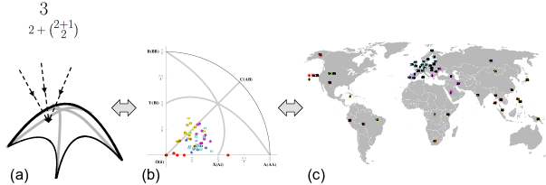
We anticipate that our analytical solutions may be a good starting basis for understanding more sophisticated models.
With the experimental evidence between the
the world-ethnic-group blood type genotype frequency data and our stable solutions, we believe that our stable solutions and exact dynamical analytic solutions
can be applied to other macroscopic population genetic systems (including human ethnic groups as well as other animals or plants), as long as the system is approximately obeying the assumptions we made.
We hope that our parameterization of analytic stable fixed-point solutions can be an efficient map to characterize the stabilized genotype frequencies. Our mapping may find its home in the textbooks of population genetics and evolutionary
biology in the future.
II Four assumptions from fundamental views
Here we start from scratch, by introducing the four fundamental assumptions used to construct our model. Our purpose lies in knowing how the genotype frequencies evolve under the mating process of a certain population system.
First, we focused on a system where the mating process is approximately closed inside itself. Hence, the newborn generation is totally a production from the old generation of the system. We should be aware that it does not matter whether the population locates together geographically. In this way, we could associate our model to different ethnic groups of humans, because the mating process of each ethnic group is approximately closed in each system. Hybrids between different ethnic groups are usually minorities compared to the majority ethnic groups.
Second, to determine the mating procedure, we assume the mating is overall average and random, which is intuitively reasonable under mean-field approximation. This assumption would not be far away from reality, considering the balance within an overall large population system. This assumption states no preference for the mating in a certain system. For example, we consider a system of genotypes. Suppose is the population amount of the genotype , and assume a half-male-half-female population. The random mating mechanism of the male amount mates with all types of the female amount is , where is the total population. We interpret this expression as the male amount multiplied by the probability to meet certain types of female. On the other hand, we have the female amount to meet all types of the male amount . Notice that the interchangeable term counts only once (male with female ); however, counts twice (male with female , and male with female ). The only mating dependence on a certain genotype is the population number of that genotype - if the population number for a certain genotype is large, then, it will have a greater chance to mate and also to be mated with by other genotype; and vice versa. Overall, this mechanism gives quadratic forms to the governing equations. The mating within the same ethnic groups or in a local geographical region plausibly obeys this second assumption.
Third, we consider the simplest inheritance law, the classical genetics: Mendelian inheritance, to relate the transmission of hereditary traits (alleles) from the parents to the newborn generation. Although there is much new progress in genetics study, Mendelian inheritance is still a primary principle for capturing the main properties of heredity.
Fourth, in order to make the system dynamic under the time evolution, there must be a guideline for population growth. Here we consider the exponential growth — Malthusian growth model. Again, this law adumbrates the main feature of population growth with some acceptable deviations from the experiment. We will find later that these assumptions are beneficial for having analytically exactly solvable solutions.
One can apply the model to other animal or plant mating systems under a similar inheritance law, if it basically satisfies the above assumptions.
We summarize our four assumptions as follows:
(a) The mating of gene-holders is (approximately) closed in a
population system.
(b) The mating probability for a certain genotype to another genotype,
due to average-and-random mating mechanism, is proportional to
the product of their population (quadratic form). It evolves under the mean-field assumption.
(c) The probability of a genotype for the newborn generation obeys the
Mendelian inheritance.
(d) The accumulation of human population obeys the exponential growth law, for both the birth and the death processes.
We should be aware of the fourth assumption that the exponential growth includes the balance between the newborn and the dead. We denote the birth rate and the death rate . The overall net growth rate is .
To derive the governing differential equations, implicitly we have another hidden assumption: the continuous limit. Throughout our work, we will take the continuous time . The discrete positive integer population number can be treated approximately as a continuous real number in a large population.
III Model
III.1 Model of 2 Alleles: 1 Dominant Gene and 1 Recessive Gene
III.1.1 Governing equations for population
We first consider the simplest model of our theory, which begins with two alleles and a single locus, such as one dominant gene and one recessive gene . We take the hairstyle being curly or straight as an example, which roughly obeys this kind of inheritance law. Dominant gene shows the curly property; only inheritance of no dominant gene shows the straight property. Curl hair owners indicate their genotype must be either or . Straight hair owners’ genotype must be . Below we denote the population parameters: for , for , and for . stands for the number of people in the population carrying , stands for the number of people in the population carrying , and stands for the number of people in the population carrying .
We now can write down the governing differential equations under a time evolution of population number for hairstyle based on 4 assumptions in Sec.II:
| (1) |
We denote the total population to be .
These equations have a first-order time derivative , associating the left-hand-side (LHS) population changes to the right-hand-side (RHS) birth and death effects. Linear terms on the RHS represent the death amount per unit time. Quadratic forms on the RHS represent the newborn population per unit time following Mendelian inheritance. Taking of , for example, it represents our second assumption that the probability for male to meet female is . The offspring of those parents is definitely . So there must be a term in the RHS of the equation , up to a constant factor. Now considering the term, it can be either male to meet female , or male to meet female . So the overall effect must be for the RHS newborn generation. The is separated into two parts: for and for , because Mendelian inheritance shows the offspring of and parents has a half probability to be and another half to be . Similarly, we can determine all the other coefficients of quadratic terms by the same arguments. The sum on the newborn part of the RHS must be all the possibilities for any pair of genes (alleles), , and this is equal to . We notice that the sum of RHS is , LHS is . This perfectly obeys assumption (d): . We next check that the model is self-consistent, and uniquely determined by our four assumptions listed in Sec.II.
III.1.2 Governing equations for percentages
Now we revise our equations via normalizing each gene carrier population by the total population, using the percentage parameters, so called genotype frequencies. Consider, , where is any one of . This turns out to be . Now by redefining , we have the governing equations for genotype frequencies:
| (2) |
We notice that the death rate takes no effect on the percentage governing equations. That is because the death effect does not rearrange the percentage parameters, every percentage parameter just universally dies away. Although the population parameter changes under death effect, the genotype frequency does not.
III.1.3 Equilibrium solutions
We should be aware that there is a constraint , and the limited range for each parameter. The total degree of freedom is . Namely the whole parameter space of population parameters are 3 dimensional, but the whole parameter space of percentage parameters, the genotype frequencies, are 2 dimensional.
Our aim is to realize the time evolution properties of this dynamical model. We first narrow down to see the equilibrium solution, which is the solution fixed in the parameter space without evolving under time evolution. The solution are solved by setting the RHS algebraic equations Eq.(2) to be zero. Among all expressions of the algebraic solution, we find the following one is the most appropriate representation:
| (3) |
It gives an one-to-one mapping between the equilibrium solution and , and shows the solution is a 1-dimensional continuous manifold. This representation also shows the symmetry of and in governing equations relates to the symmetry of and in equilibrium solution. The symmetry of relates to the S2 symmetry of . The S2 symmetry also results in a number of time-independent conserved quantities under Eq.(2). We find, for example, . By the constraint , the three quantities , , and are indeed the same equivalent conserved quantity. We can say the S2 symmetry results in 1 conserved quantity, thus the dimensionality of fixed-point solutions is 1, here parametrized by .
III.1.4 From the linear stability analysis to the exact analytic time-dependent dynamical solution
By doing the linear stability analysis on the dynamical Eq.(2) with a small perturbation around this equilibrium solution Eq.(3), we find that it is stable with eigenvalues , RG for the entire two-dimensional parameter space. The first eigenvector for the eigenvalue 0 corresponds to the marginal tangent direction RG of -dimensional equilibrium solution. Surprisingly, the second eigenvector for the eigenvalue 1 is irrelevant and stable perturbation RG along the fixed direction . We define a new basis , and is the coordinate along
It is well-known that nonlinear equations may have complicated global properties, such as chaotic behaviors. Usually the numerical simulation is required, and there are seldom cases which analytic solution for time evolution is exactly solvable. However, below we will show how to obtain the exact analytic time-dependent solution of Eq.(2). Our method is to change the description of parameters in Cartesian coordinates to parameters in curvilinear coordinates . We transform to by the following:
| (4) |
The transformation is well-defined for a 2-dimensional one-to-one mapping with an inverse function:
| (5) |
We could substitute this inverse transformation into the equilibrium solution Eq.(3) to obtain the equilibrium solution as the parameterizations of :
| (6) |
This indicates two lessons. First, once we know the original set of genotype frequencies as the initial condition, remarkably we can deduce the final equilibrium . Second, and , these two numbers determine the final equilibrium. This implies, for the same number set of and , even for different , their final equilibriums are the same.
Substituting the reparameterization Eq.(4) to the governing equations Eq.(2), this not only decouples the parameters, but also decodes the equations to one time-dependent equation and the other time-independent equation:
| (7) |
Both are exactly solvable. Remarkably, we have transformed the nonlinear coupled differential equations Eq.(2) to the linear decoupled differential equations Eq.(7).
We foresee in advance the equilibrium solution is a global attractor, attracting all the points on the line direction of a certain given initial to the equilibrium point of the same in the exponential decay way along the direction. Because each line direction for a is independent to each other with no intersection, this makes our solution well-defined everywhere in the parameter space. The global picture of time evolution is: giving any initial value in the parameter space, there is only one corresponding with a line direction of connecting that equilibrium point to the initial value; the time evolution of parameters will go along the line direction to the equilibrium point in the exponential decay to reduce the distance away from the equilibrium point.
The method for deriving the analytic solution is the following: for any given initial value and find the corresponding set of By Eq.,We then have . Because the transformation between old and new coordinate is well-defined, we can further solve the new equations and replace the parameters from to by Eq.(5).
Hence, we achieve our exact analytic solution:
| (8) |
The illustration of Eq.(8) is shown in Fig.3. The equilibrium solutions coincide with the De Finetti diagram book2 .
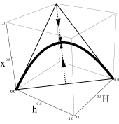
Intuitively we would like to compare this model and its analytic solution to experimental numerical data. It will be more appropriate to fit the experimental data into the equilibrium solution, because we can imagine that the genotype frequencies have been more-or-less stabilized within a closed population under the sufficient amount of time-evolution.
For this 1-Dominant-Gene-and-1-Recessive-Gene (hairstyle) model, the observables of available experimental data are the phenotypes, the representative biological characters, of curl ( and ) and straight () hairs. The two phenotype frequencies with one constraint, has 1 degree of freedom; this is the same as the 1 degree of freedom of the continuous equilibrium solution. The fitting can be perfectly with no error bar; however, this is due to the same degree of freedom of correspondence, rather than the evidence of successful description of this model. Hence, the hairstyle experimental data cannot illustrate the validity of the theory.
In the next, we shall turn to the next-simplest model: 3 alleles, such as 2 dominant genes and 1 recessive gene case, for example, the blood-type model, to check the experimental evidence of our theory.
III.2 Model of 3 Alleles: 2 Dominant Genes and 1 Recessive Gene: Blood Type Evolution Model
III.2.1 Governing equations and exact analytic solutions
For the model of 3 alleles, such as two dominant genes , and one recessive gene of blood types, the
representative phenotypes are type A: and , type B: and , type AB: , and type O: .
There are four kinds of representative phenotypes (A, B, AB, O), and six parameters of genotype population , for a total population . Here we follow the similar derivation as the previous model in Sec III.1. to write down the governing equations for the population parameters:
| (9) |
By redefining as the percentage parameters, where is any of the six parameters, we can derive the governing percentage parameters equations for genotype frequencies:
| (10) |
Now, we generalize the equilibrium solution (3) of Eq.(2) to the equilibrium solution of Eq.(10):
| (11) |
We can further make the above 2-dimensional equilibrium parameterization an one-to-one mapping to , if we define that shrinks into a point. Namely, can be a well-defined one-to-one reparameterization of the equilibrium solution Eq.(11).
The linear stability analysis shows this system is again locally stable with five eigenvalues RG . Here two eigenvalues correspond to two eigenvectors along the marginal tangent plane RG of 2-dimensional equilibrium solutions, three eigenvalues correspond to the stable perturbation RG along the three eigenvectors , , . Defining those eigenvectors as with coordinates , we could transform of the whole parameter space (6-dimensions with 1 constraint ) to a set of 5-dimensional new coordinates :
| (12) |
We have the following inverse function:
| (13) |
Substitute the reparameterization Eq.(12) to Eq.(10), we confirm again this system will be global stable like the previous model in Sec.III.1.
| (14) |
The analytic solution is determined by a given set of initial values which correspond to a set of via Eq.(13). We obtain the exact analytic time-dependent dynamical solution:
| (15) |
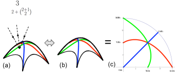
The dimensionality: We shall explain the physical meaning on the dimensionality of the fibers and the stable base manifold. For both Eq.(9) and Eq.(10), there is a permutation symmetric group S3 symmetry by exchanging , , and their corresponding genotypes. The S3 symmetry also results in time-independent conserved quantities, spanned by , and , with a constraint . There are totally 2 independent degrees of freedom. We can say the S3 symmetry results in the dimensionality of fixed-point solutions is 2, here parametrized by .
III.2.2 Experimental evidence - data fitting
As we mentioned, we would like to fit the available blood type data - blood type population percentages as genotype frequencies of any ethnic group, into our equilibrium solutions on the stable 2-dimensional manifold of Eq.(11). For a set of genotype frequencies , it totally forms a set of 5-dimensional degrees of freedom (due to 6 numbers with 1 constraint). We could correlate this with for a 2-dimensional parameterization . In this way, there would be a correspondence between 5-dimensions and 2-dimensions, the validity of experimental fitness to our theoretical prediction would be a strong evidence for the validity of our model. However, current available experimental data we found is just (Oexp,Aexp,Bexp,ABexp), which is 3-dimensional (4 numbers with 1 constraint) ; we would then correlate this to for certain 2-dimensional parameters . The test for the validity of this theory now becomes a correspondence between 3-dimensions to 2-dimensions. We fit the 3-dimensional experimental data into our 2-dimensional equilibrium solutions. Although this is not as stringent as the 5-dimensional to 2-dimensional correspondence, there remains one degree of freedom for experimental data to deviate from our equilibrium solution. If the error bar for this 3-dimensional to 2-dimensional correspondence is tiny, then our theory shows consistency to the level of predicting the stability of genotype frequencies.
Our fitting procedure is to solve from two equalities:
| (16) |
Then, with applicable as solutions of equalities, we can further know Ot and ABt. Since AAt and BBt by Eq.(16), we could test the differences and error bars of O and AB as follows:
| (17) |
As we mention the 2-dimensional equilibrium parameterization is an one-to-one mapping if we define that shrinks into a point. Hence, we can introduce the polar coordinates mapped from the Eq.(11) of the parameter . In other words, we define that represents the radial direction, represents the angle direction for our stable equilibrium solution diagram, show in FIG.5 as our blood type mapping chart. This chart is a quadrant: one fourth of a circle. Inside the quadrant consists of all stable fixed points mapping from the 2-dimensional manifold Eq.(11). At three corners of the quadrant, there are oO(ii), aA(AA), and bB(BB). For specifying their Cartesian coordinates , each of these is of that specified type - e.g. O(ii) , A(AA) , B(BB) . Similarly, at the midpoints of the three edge sides, we have X(Ai) , Y(Bi) , and C(AB) . The blue line represents the symmetric line invariant under switching to .
From Eq.(11), we could easily see the blue line is . The green curve represents the symmetry invariant under switching to . This gives the green curve parameterization:
| (18) |
The red curve represents the symmetry invariant under switching to . This gives the red curve parameterization:
| (19) |
The intersection of three color lines, is , which is the most symmetric mid point.
III.2.3 Explanation and application of the chart - relations of different ethnic groups by geodesic distances
The experimental data that we implemented is mainly from two data resources data . We fit the experimental data data for both (1) different ethnic groups and (2) different countries.
We present the experimental data (Oexp,Aexp,Bexp,ABexp)
in Table.1, 3, 4.
We present our corresponding theoretical prediction, the data (Ot,AAt, Ait,BBt,Bit,ABi) in
Table.2, 5, 6.
Data fitting for ethnic groups is much promising, because random mating assumption is approximately true for a certain given ethnic group. On the other hand, a country may possess multi-ethnicities where the random mating assumption generally fails for the country with multi-ethnic groups.
We also investigate the data distribution of different ethnic groups and countries under our domain space. We found some facts:
(1) American aboriginals possess large portion of Type O.
(2) Europeans or Caucasians possess much more Type A than others.
(3) Mongolians, like Buryats, possess comparably more Type B.
(4) Diff% and Error% for islanders, like Irish and Japanese,
are smaller than races living in a larger continent, like Hindus.
Thus, we can say that the closed system assumption plays an important rule
such that the data of islanders are more close to the stable fixed-point equilibrium solutions.
In our plots (see Figures in Sec.VIII), represents the radial direction , represents the angle direction . We invent the chart to organize the data - for the blood type model, we have a quadrant spanned by and with the horizontal and vertical coordinates as . We propose the distribution of different ethnic groups (marked with numbers) in our plots would reveal their relative distance correlations. More precisely, to quantitatively define the distance between two ethnic groups, we propose a mathematical method to achieve this by solving the geodesic equation numerically from the given metric of stable-solution manifold.
For the model of 2 alleles studied here in Sec.III.1, we can write down the intrinsic metric of 1-dimensional equilibrium manifold Eq.(3). This can be done by considering the infinitesimal distance in the genotype frequency space by transforming the Euclidean space to the curved space :
| (20) |
For example, for the model of 3 alleles studied in Sec.III.2, we can write down the intrinsic metric of 2-dimensional equilibrium manifold Eq.(11). This can be done by considering the infinitesimal distance in the genotype frequency space by transforming the Euclidean space to the curved space :
| (21) |
where in the second line all the parameters are re-written in terms of , e.g.
, etc.
We propose that:
The genetic distance between two ethnic groups with stabilized genotype frequencies
can be defined as the geodesic length by solving the geodesic equation
on the stable equilibrium manifold.
On one hand, we could further define this least distance as the “genetic distance” between any pair of two ethnic groups. On the other hand, by comparing the geographical distribution of ethnic groups and the distribution of ethnic groups on our equilibrium-solution chart, we find their strong correlation and certain meaningful pattern. The details of the data of geodesic distance shall be left for the future.
| Index | Ethnic (People Group) | Oexp(%) | Aexp(%) | Bexp(%) | ABexp(%) | Diff%(Ot-Oexp) | Diff%(ABt-ABexp) | ||
|---|---|---|---|---|---|---|---|---|---|
| 1 | Aborigines | 61 | 39 | 0 | 0 | 0.2734 | 0.0000 | 0.0000 | 0.0000 |
| 2 | Abyssinians | 43 | 27 | 25 | 5 | 0.5011 | 0.7511 | -1.2547 | 1.2547 |
| 3 | Albanians | 38 | 43 | 13 | 6 | 0.5487 | 0.3314 | 0.5169 | -0.5169 |
| 4 | Arabs | 34 | 31 | 29 | 6 | 0.6971 | 0.7570 | -4.3754 | 4.3754 |
| 5 | Armenians | 31 | 50 | 13 | 6 | 0.7012 | 0.3027 | -1.6005 | 1.6005 |
| 6 | Asian(USA) | 40 | 28 | 27 | 5 | 0.5646 | 0.7694 | -2.5159 | 2.5159 |
| 7 | Bantus | 46 | 30 | 19 | 5 | 0.4423 | 0.5843 | 0.0498 | -0.0498 |
| 8 | Basques | 51 | 44 | 4 | 1 | 0.3860 | 0.1052 | -0.4424 | 0.4424 |
| 9 | Belgians | 47 | 42 | 8 | 3 | 0.4285 | 0.2140 | 0.1153 | -0.1153 |
| 10 | Blackfoot(N. Am. Indian) | 17 | 82 | 0 | 1 | 0.9357 | 0.0000 | 1.0000 | -1.0000 |
| 11 | Bororo | 100 | 0 | 0 | 0 | 0.0000 | 0.0000 | 0.0000 | |
| 12 | Brazilians | 47 | 41 | 9 | 3 | 0.4323 | 0.2437 | -0.1799 | 0.1799 |
| 13 | Burmese | 36 | 24 | 33 | 7 | 0.6087 | 0.9224 | -1.2738 | 1.2738 |
| 14 | Buryats | 33 | 21 | 38 | 8 | 0.6504 | 1.0313 | -0.7470 | 0.7470 |
| 15 | Chinese-Canton | 46 | 23 | 25 | 6 | 0.4290 | 0.8232 | 1.0825 | -1.0825 |
| 16 | Danes | 41 | 44 | 11 | 4 | 0.5206 | 0.2798 | -0.6050 | 0.6050 |
| 17 | Dutch | 45 | 43 | 9 | 3 | 0.4622 | 0.2354 | -0.4505 | 0.4505 |
| 18 | Eskimos(Alaska) | 38 | 44 | 13 | 5 | 0.5680 | 0.3264 | -0.7347 | 0.7347 |
| 19 | Finns | 34 | 41 | 18 | 7 | 0.6372 | 0.4546 | -0.9803 | 0.9803 |
| 20 | French | 43 | 47 | 7 | 3 | 0.4836 | 0.1736 | -0.0098 | 0.0098 |
| 21 | Germans | 41 | 43 | 11 | 5 | 0.5034 | 0.2842 | 0.5868 | -0.5868 |
| 22 | Hindus(Bombay) | 32 | 29 | 28 | 11 | 0.6127 | 0.7701 | 2.4826 | -2.4826 |
| 23 | Hungarians | 36 | 43 | 16 | 5 | 0.6267 | 0.3990 | -2.3598 | 2.3598 |
| 24 | Indians(USA) | 79 | 16 | 4 | 1 | 0.1201 | 0.2532 | 0.6212 | -0.6212 |
| 25 | Irish | 52 | 35 | 10 | 3 | 0.3667 | 0.3035 | 0.2035 | -0.2035 |
| 26 | Japanese | 30 | 38 | 22 | 10 | 0.6810 | 0.5591 | 0.5134 | -0.5134 |
| 27 | Jews(Germany) | 42 | 41 | 12 | 5 | 0.4907 | 0.3184 | 0.4772 | -0.4772 |
| 28 | Jews(Poland) | 33 | 41 | 18 | 8 | 0.6372 | 0.4546 | 0.0197 | -0.0197 |
| 29 | Kikuyu(Kenya) | 60 | 19 | 20 | 1 | 0.3015 | 0.8093 | -1.8112 | 1.8112 |
| 30 | Lapps | 29 | 63 | 4 | 4 | 0.6892 | 0.0847 | 1.0566 | -1.0566 |
| 31 | Latvians | 32 | 37 | 24 | 7 | 0.7180 | 0.6056 | -3.5096 | 3.5096 |
| 32 | Lithuanians | 40 | 34 | 20 | 6 | 0.5345 | 0.5582 | -0.5444 | 0.5444 |
| 33 | Malasians | 62 | 18 | 20 | 0 | 0.2894 | 0.8346 | -2.6261 | 2.6261 |
| 34 | Moros | 64 | 16 | 20 | 0 | 0.2663 | 0.8895 | -2.2717 | 2.2717 |
| 35 | Navajo(N. Am. Indain) | 73 | 27 | 0 | 0 | 0.1688 | 0.0000 | 0.0000 | 0.0000 |
| 36 | Papuas(New Guinea) | 41 | 27 | 23 | 9 | 0.4631 | 0.7135 | 3.4828 | -3.4828 |
| 37 | Persians | 38 | 33 | 22 | 7 | 0.5594 | 0.6103 | -0.1801 | 0.1801 |
| 38 | Peru(Indians) | 100 | 0 | 0 | 0 | 0.0000 | 0.0000 | 0.0000 | |
| 39 | Philippinos | 45 | 22 | 27 | 6 | 0.4452 | 0.8774 | 0.8265 | -0.8265 |
| 40 | Portuguese | 35 | 53 | 8 | 4 | 0.6123 | 0.1834 | -0.4928 | 0.4928 |
| 41 | Rumanians | 34 | 41 | 19 | 6 | 0.6673 | 0.4755 | -2.7138 | 2.7138 |
| 42 | Russians | 33 | 36 | 23 | 8 | 0.6572 | 0.5969 | -1.1401 | 1.1401 |
| 43 | Sardinians | 50 | 26 | 19 | 5 | 0.3808 | 0.6435 | 0.9971 | -0.9971 |
| 44 | Scotts | 51 | 34 | 12 | 3 | 0.3846 | 0.3659 | -0.3254 | 0.3254 |
| 45 | Shompen(Nicobars) | 100 | 0 | 0 | 0 | 0.0000 | 0.0000 | 0.0000 | |
| 46 | Slovaks | 42 | 37 | 16 | 5 | 0.5049 | 0.4409 | -0.5190 | 0.5190 |
| 47 | South Africans | 45 | 40 | 11 | 4 | 0.4547 | 0.2993 | 0.1149 | -0.1149 |
| 48 | Spanish | 38 | 47 | 10 | 5 | 0.5510 | 0.2447 | 0.3680 | -0.3680 |
| 49 | Swedes | 38 | 47 | 10 | 5 | 0.5510 | 0.2447 | 0.3680 | -0.3680 |
| 50 | Swiss | 40 | 50 | 7 | 3 | 0.5321 | 0.1666 | -0.3848 | 0.3849 |
| 51 | Tartars | 28 | 30 | 29 | 13 | 0.6671 | 0.7708 | 3.2975 | -3.2975 |
| 52 | Thais | 37 | 22 | 33 | 8 | 0.5594 | 0.9605 | 0.8199 | -0.8199 |
| 53 | United Kingdom(GB) | 47 | 42 | 8 | 3 | 0.4285 | 0.2140 | 0.1153 | -0.1153 |
| 54 | USA(blacks) | 49 | 27 | 20 | 4 | 0.4114 | 0.6504 | -0.5293 | 0.5293 |
| 55 | USA(whites) | 45 | 40 | 11 | 4 | 0.4547 | 0.2993 | 0.1149 | -0.1149 |
| Index | Ethnic (People Group) | Ot(%) | AAt(%) | Ait(%) | BBt(%) | Bit(%) | ABt(%) | Error%() | Error%() |
|---|---|---|---|---|---|---|---|---|---|
| 1 | Aborigines | 61.00 | 4.80 | 34.21 | 0.00 | 0.00 | 0.00 | 0.00 | |
| 2 | Abyssinians | 41.75 | 3.35 | 23.65 | 2.92 | 22.08 | 6.25 | -2.92 | 25.09 |
| 3 | Albanians | 38.52 | 7.97 | 35.03 | 0.94 | 12.06 | 5.48 | 1.36 | -8.62 |
| 4 | Arabs | 29.62 | 5.49 | 25.51 | 4.90 | 24.10 | 10.38 | -12.87 | 72.92 |
| 5 | Armenians | 29.40 | 12.17 | 37.83 | 1.19 | 11.81 | 7.60 | -5.16 | 26.67 |
| 6 | Asian(USA) | 37.48 | 3.88 | 24.12 | 3.64 | 23.36 | 7.52 | -6.29 | 50.32 |
| 7 | Bantus | 46.05 | 3.74 | 26.26 | 1.64 | 17.36 | 4.95 | 0.11 | -1.00 |
| 8 | Basques | 50.56 | 6.83 | 37.17 | 0.08 | 3.92 | 1.44 | -0.87 | 44.24 |
| 9 | Belgians | 47.12 | 6.64 | 35.36 | 0.31 | 7.69 | 2.88 | 0.25 | -3.84 |
| 10 | Blackfoot(N. Am. Indian) | 18.00 | 33.15 | 48.85 | 0.00 | 0.00 | 0.00 | 5.88 | -100.00 |
| 11 | Bororo | 100.00 | 0.00 | 0.00 | 0.00 | 0.00 | 0.00 | 0.00 | |
| 12 | Brazilians | 46.82 | 6.39 | 34.61 | 0.40 | 8.60 | 3.18 | -0.38 | 6.00 |
| 13 | Burmese | 34.73 | 3.13 | 20.87 | 5.46 | 27.54 | 8.27 | -3.54 | 18.20 |
| 14 | Buryats | 32.25 | 2.62 | 18.38 | 7.30 | 30.70 | 8.75 | -2.26 | 9.34 |
| 15 | Chinese-Canton | 47.08 | 2.28 | 20.72 | 2.65 | 22.35 | 4.92 | 2.35 | -18.04 |
| 16 | Danes | 40.40 | 8.01 | 35.99 | 0.66 | 10.34 | 4.60 | -1.48 | 15.12 |
| 17 | Dutch | 44.55 | 7.19 | 35.81 | 0.41 | 8.59 | 3.45 | -1.00 | 15.02 |
| 18 | Eskimos(Alaska) | 37.27 | 8.47 | 35.53 | 0.97 | 12.03 | 5.73 | -1.93 | 14.69 |
| 19 | Finns | 33.02 | 8.16 | 32.84 | 1.95 | 16.05 | 7.98 | -2.88 | 14.00 |
| 20 | French | 42.99 | 8.58 | 38.42 | 0.26 | 6.74 | 3.01 | -0.02 | 0.33 |
| 21 | Germans | 41.59 | 7.55 | 35.45 | 0.64 | 10.36 | 4.41 | 1.43 | -11.74 |
| 22 | Hindus(Bombay) | 34.48 | 4.39 | 24.61 | 4.13 | 23.87 | 8.52 | 7.76 | -22.57 |
| 23 | Hungarians | 33.64 | 8.73 | 34.27 | 1.55 | 14.45 | 7.36 | -6.56 | 47.20 |
| 24 | Indians(USA) | 79.62 | 0.73 | 15.27 | 0.05 | 3.95 | 0.38 | 0.79 | -62.12 |
| 25 | Irish | 52.20 | 4.47 | 30.53 | 0.44 | 9.56 | 2.80 | 0.39 | -6.78 |
| 26 | Japanese | 30.51 | 7.58 | 30.42 | 2.97 | 19.03 | 9.49 | 1.71 | -5.13 |
| 27 | Jews(Germany) | 42.48 | 6.86 | 34.14 | 0.75 | 11.25 | 4.52 | 1.14 | -9.54 |
| 28 | Jews(Poland) | 33.02 | 8.16 | 32.84 | 1.95 | 16.05 | 7.98 | 0.06 | -0.25 |
| 29 | Kikuyu(Kenya) | 58.19 | 1.34 | 17.66 | 1.47 | 18.53 | 2.81 | -3.02 | 181.12 |
| 30 | Lapps | 30.06 | 17.34 | 45.66 | 0.12 | 3.88 | 2.94 | 3.64 | -26.42 |
| 31 | Latvians | 28.49 | 7.59 | 29.41 | 3.64 | 20.36 | 10.51 | -10.97 | 50.14 |
| 32 | Lithuanians | 39.46 | 5.24 | 28.76 | 2.04 | 17.96 | 6.54 | -1.36 | 9.07 |
| 33 | Malasians | 59.37 | 1.19 | 16.81 | 1.45 | 18.55 | 2.63 | -4.24 | |
| 34 | Moros | 61.73 | 0.92 | 15.08 | 1.40 | 18.60 | 2.27 | -3.55 | |
| 35 | Navajo(N. Am. Indain) | 73.00 | 2.12 | 24.88 | 0.00 | 0.00 | 0.00 | 0.00 | |
| 36 | Papuas(New Guinea) | 44.48 | 3.19 | 23.81 | 2.39 | 20.61 | 5.52 | 8.49 | -38.70 |
| 37 | Persians | 37.82 | 5.13 | 27.87 | 2.51 | 19.49 | 7.18 | -0.47 | 2.57 |
| 38 | Peru(Indians) | 100.00 | 0.00 | 0.00 | 0.00 | 0.00 | 0.00 | 0.00 | |
| 39 | Philippinos | 45.83 | 2.15 | 19.85 | 3.11 | 23.89 | 5.17 | 1.84 | -13.77 |
| 40 | Portuguese | 34.51 | 12.11 | 40.89 | 0.42 | 7.58 | 4.49 | -1.41 | 12.32 |
| 41 | Rumanians | 31.29 | 8.46 | 32.54 | 2.24 | 16.76 | 8.71 | -7.98 | 45.23 |
| 42 | Russians | 31.86 | 6.72 | 29.28 | 3.11 | 19.89 | 9.14 | -3.45 | 14.25 |
| 43 | Sardinians | 51.00 | 2.67 | 23.33 | 1.50 | 17.50 | 4.00 | 1.99 | -19.94 |
| 44 | Scotts | 50.67 | 4.34 | 29.66 | 0.64 | 11.36 | 3.33 | -0.64 | 10.85 |
| 45 | Shompen(Nicobars) | 100.00 | 0.00 | 0.00 | 0.00 | 0.00 | 0.00 | 0.00 | |
| 46 | Slovaks | 41.48 | 5.85 | 31.15 | 1.30 | 14.70 | 5.52 | -1.24 | 10.38 |
| 47 | South Africans | 45.11 | 6.30 | 33.70 | 0.60 | 10.40 | 3.89 | 0.26 | -2.87 |
| 48 | Spanish | 38.37 | 9.27 | 37.73 | 0.58 | 9.42 | 4.63 | 0.97 | -7.36 |
| 49 | Swedes | 38.37 | 9.27 | 37.73 | 0.58 | 9.42 | 4.63 | 0.97 | -7.36 |
| 50 | Swiss | 39.62 | 10.06 | 39.94 | 0.28 | 6.72 | 3.38 | -0.96 | 12.83 |
| 51 | Tartars | 31.30 | 4.99 | 25.01 | 4.71 | 24.29 | 9.70 | 11.78 | -25.37 |
| 52 | Thais | 37.82 | 2.51 | 19.49 | 5.13 | 27.87 | 7.18 | 2.22 | -10.25 |
| 53 | United Kingdom(GB) | 47.12 | 6.64 | 35.36 | 0.31 | 7.69 | 2.88 | 0.25 | -3.84 |
| 54 | USA(blacks) | 48.47 | 2.98 | 24.02 | 1.72 | 18.28 | 4.53 | -1.08 | 13.23 |
| 55 | USA(whites) | 45.11 | 6.30 | 33.70 | 0.60 | 10.40 | 3.89 | 0.26 | -2.87 |
| Index | Country | Oexp(%) | Aexp(%) | Bexp(%) | ABexp(%) | Diff%(Ot-Oexp) | Diff%(ABt-ABexp) | ||
|---|---|---|---|---|---|---|---|---|---|
| 1 | Canada | 41 | 45 | 10 | 4 | 0.5156 | 0.2519 | -0.2600 | 0.2600 |
| 2 | USA | 45 | 41 | 10 | 4 | 0.4510 | 0.2691 | 0.3930 | -0.3930 |
| 3 | Mexico | 84 | 11 | 4 | 1 | 0.0860 | 0.3550 | 0.7512 | -0.7512 |
| 4 | Guatemala | 95 | 3 | 2 | 0 | 0.0261 | 0.5892 | -0.0312 | 0.0312 |
| 5 | El Salvador | 60 | 26 | 11 | 3 | 0.2738 | 0.4187 | 0.9503 | -0.9503 |
| 6 | Nicaragua | 92 | 7 | 1 | 0 | 0.2738 | 0.1441 | -0.0373 | 0.0373 |
| 7 | Costa Rica | 53 | 31 | 13 | 3 | 0.3597 | 0.4210 | -0.1914 | 0.1914 |
| 8 | Cuba | 49 | 36 | 12 | 3 | 0.4128 | 0.3503 | -0.6358 | 0.6358 |
| 9 | Jamaica | 56 | 20 | 21 | 3 | 0.3266 | 0.8080 | -0.1988 | 0.1988 |
| 10 | Dominican Rep | 53 | 31 | 13 | 3 | 0.3597 | 0.4210 | -0.1914 | 0.1914 |
| 11 | Haiti | 51 | 27 | 18 | 4 | 0.3800 | 0.6035 | 0.0651 | -0.0651 |
| 12 | Puerto Rico | 47 | 30 | 13 | 10 | 0.3468 | 0.4317 | 6.9573 | -6.9573 |
| 13 | Colombia | 62 | 27 | 9 | 2 | 0.2610 | 0.3401 | 0.2843 | -0.2843 |
| 14 | Ecuador | 63 | 29 | 6 | 2 | 0.2469 | 0.2195 | 0.7914 | -0.7914 |
| 15 | Peru | 71 | 19 | 9 | 1 | 0.1855 | 0.4544 | -0.1006 | 0.1006 |
| 16 | Chile | 56 | 31 | 10 | 3 | 0.3174 | 0.3342 | 0.6607 | -0.6607 |
| 17 | Bolivea | 93 | 5 | 2 | 0 | 0.0372 | 0.3832 | -0.0528 | 0.0528 |
| 18 | Venezuela | 44 | 37 | 14 | 5 | 0.4645 | 0.3933 | 0.3814 | -0.3814 |
| 19 | Brazil | 48 | 39 | 10 | 3 | 0.4213 | 0.2793 | -0.3173 | 0.3173 |
| 20 | Argentina | 48 | 39 | 10 | 3 | 0.4213 | 0.2793 | -0.3173 | 0.3173 |
| 21 | Paraguay | 56 | 34 | 9 | 1 | 0.3393 | 0.2818 | -1.3696 | 1.3696 |
| 22 | Uruguay | 45 | 42 | 10 | 3 | 0.4664 | 0.2644 | -0.7603 | 0.7603 |
| 23 | Australia | 47 | 40 | 10 | 3 | 0.4359 | 0.2740 | -0.4594 | 0.4594 |
| 24 | New Zealand | 48 | 40 | 9 | 3 | 0.4180 | 0.2483 | -0.0520 | 0.0520 |
| 25 | Iceland | 56 | 32 | 10 | 2 | 0.3293 | 0.3258 | -0.4484 | 0.4484 |
| 26 | Ireland | 54 | 33 | 10 | 3 | 0.3414 | 0.3179 | 0.4391 | -0.4391 |
| 27 | United Kingdom | 47 | 41 | 9 | 3 | 0.4323 | 0.2437 | -0.1799 | 0.1799 |
| 28 | Scotland | 51 | 35 | 11 | 3 | 0.3823 | 0.3310 | -0.1307 | 0.1307 |
| 29 | England | 46 | 43 | 8 | 3 | 0.4430 | 0.2103 | -0.0025 | 0.0025 |
| 30 | Norway | 39 | 49 | 8 | 4 | 0.5386 | 0.1922 | 0.1844 | -0.1844 |
| 31 | Sweden | 38 | 47 | 10 | 5 | 0.5510 | 0.2447 | 0.3680 | -0.3680 |
| 32 | Finland | 33 | 42 | 18 | 7 | 0.6619 | 0.4480 | -1.4095 | 1.4095 |
| 33 | Denmark | 42 | 44 | 10 | 4 | 0.4987 | 0.2558 | -0.0863 | 0.0863 |
| 34 | Netherland | 45 | 43 | 9 | 3 | 0.4622 | 0.2354 | -0.4505 | 0.4505 |
| 35 | Belgium | 46 | 43 | 8 | 3 | 0.4430 | 0.2103 | -0.0025 | 0.0025 |
| 36 | France | 43 | 45 | 9 | 3 | 0.4938 | 0.2279 | -0.7431 | 0.7431 |
| 37 | Spain | 42 | 45 | 9 | 4 | 0.4938 | 0.2279 | 0.2569 | -0.2569 |
| 38 | Portugal | 41 | 48 | 8 | 3 | 0.5215 | 0.1948 | -0.6655 | 0.6655 |
| 39 | Germany | 38 | 43 | 13 | 6 | 0.5487 | 0.3314 | 0.5169 | -0.5169 |
| 40 | Austria | 39 | 44 | 13 | 4 | 0.5680 | 0.3264 | -1.7347 | 1.7347 |
| 41 | Swiss | 42 | 47 | 8 | 3 | 0.5049 | 0.1976 | -0.5218 | 0.5218 |
| 42 | Italy | 45 | 40 | 11 | 4 | 0.4547 | 0.2993 | 0.1149 | -0.1149 |
| 43 | North Italy | 42 | 43 | 11 | 4 | 0.5034 | 0.2842 | -0.4132 | 0.4132 |
| 44 | South Italy | 46 | 35 | 15 | 4 | 0.4510 | 0.4343 | -0.6086 | 0.6086 |
| 45 | Czech | 33 | 41 | 18 | 8 | 0.6372 | 0.4546 | 0.0197 | -0.0197 |
| 46 | Hungary | 30 | 43 | 19 | 8 | 0.7223 | 0.4626 | -1.7437 | 1.7437 |
| 47 | *Gypsies | 30 | 25 | 36 | 9 | 0.7213 | 0.9376 | -1.6902 | 1.6902 |
| 48 | Poland | 35 | 38 | 19 | 8 | 0.5951 | 0.4987 | 0.5608 | -0.5608 |
| 49 | Yogoslavia | 37 | 42 | 14 | 7 | 0.5534 | 0.3600 | 1.2048 | -1.2048 |
| 50 | Romania | 34 | 45 | 17 | 7 | 0.7083 | 0.4097 | -4.9869 | 1.9869 |
| 51 | Bulgalia | 32 | 44 | 16 | 8 | 0.6502 | 0.3934 | 0.2636 | -0.2636 |
| 52 | Albania | 42 | 36 | 17 | 5 | 0.5078 | 0.4725 | -0.7220 | 0.7220 |
| 53 | Greece | 43 | 39 | 13 | 5 | 0.4778 | 0.3547 | 0.4094 | -0.4094 |
| 54 | Cyprus | 35 | 46 | 13 | 6 | 0.6088 | 0.3174 | -0.2807 | 0.2807 |
| 55 | Turkey | 33 | 45 | 15 | 7 | 0.6439 | 0.3665 | -0.3693 | 0.3693 |
| 56 | Iran(Westnorth) | 36 | 33 | 24 | 7 | 0.6087 | 0.6484 | -1.2738 | 1.2738 |
| 57 | Iran(Eastsouth) | 42 | 26 | 25 | 7 | 0.4820 | 0.7678 | 1.1033 | -1.1033 |
| 58 | Iran(Middleeast) | 31 | 25 | 34 | 10 | 0.6623 | 0.9162 | 0.5671 | -0.5671 |
| 59 | Iraq | 35 | 31 | 26 | 8 | 0.6115 | 0.7091 | -0.4441 | 0.4441 |
| 60 | Kuwait | 47 | 24 | 24 | 5 | 0.4291 | 0.7854 | 0.0733 | -0.0733 |
| 61 | Lebanon | 36 | 47 | 12 | 5 | 0.6023 | 0.2907 | -0.8845 | 0.8845 |
| 62 | Israel | 36 | 41 | 17 | 6 | 0.6092 | 0.4332 | -1.3042 | 1.3042 |
| Index | Country | Oexp(%) | Aexp(%) | Bexp(%) | ABexp(%) | Diff%(Ot-Oexp) | Diff%(ABt-ABexp) | ||
|---|---|---|---|---|---|---|---|---|---|
| 63 | Pakistan | 31 | 25 | 34 | 10 | 0.6623 | 0.9162 | 0.5671 | -0.5671 |
| 64 | Afgjanistan | 29 | 25 | 36 | 10 | 0.7213 | 0.9376 | -0.6902 | 0.6902 |
| 65 | India(Westnorth) | 29 | 21 | 41 | 9 | 0.7349 | 1.0549 | -1.4084 | 1.4084 |
| 66 | India(Eastnorth) | 32 | 25 | 36 | 7 | 0.7213 | 0.9376 | -3.6902 | 3.6902 |
| 67 | India(Middlesouth) | 37 | 22 | 34 | 7 | 0.5813 | 0.9719 | -0.5815 | 0.5815 |
| 68 | Srilanka | 47 | 22 | 26 | 5 | 0.4286 | 0.8609 | 0.1098 | -0.1098 |
| 69 | Myanmar | 35 | 25 | 32 | 8 | 0.6103 | 0.8921 | -0.3710 | 0.3710 |
| 70 | Thailand | 39 | 22 | 33 | 6 | 0.5594 | 0.9605 | -1.1801 | 1.1801 |
| 71 | Malaysia | 38 | 25 | 29 | 8 | 0.5418 | 0.8508 | 0.9718 | -0.9718 |
| 72 | Philippines | 45 | 26 | 24 | 5 | 0.4635 | 0.7494 | -0.5460 | 0.5460 |
| 73 | Vietnam | 42 | 22 | 31 | 5 | 0.5183 | 0.9357 | -1.4429 | 1.4429 |
| 74 | Cambodia | 39 | 23 | 35 | 3 | 0.6313 | 0.9636 | -5.6284 | 5.6284 |
| 75 | South China | 44 | 27 | 23 | 6 | 0.4631 | 0.7135 | 0.4828 | -0.4828 |
| 76 | North China | 33 | 30 | 29 | 8 | 0.6671 | 0.7708 | -1.7025 | 1.7025 |
| 77 | Middle China | 35 | 32 | 26 | 7 | 0.6371 | 0.6960 | -1.9711 | 1.9711 |
| 78 | Hong Kong | 44 | 24 | 26 | 6 | 0.4635 | 0.8214 | 0.4540 | -0.4540 |
| 79 | Macao | 40 | 25 | 28 | 7 | 0.5210 | 0.8357 | 0.3689 | -0.3689 |
| 80 | Tibet | 30 | 37 | 24 | 9 | 0.7180 | 0.6056 | -1.5096 | 1.5096 |
| 81 | Taiwan | 44 | 27 | 23 | 6 | 0.4631 | 0.7135 | 0.4828 | -0.4828 |
| 82 | Nepal | 30 | 37 | 24 | 9 | 0.7180 | 0.6056 | -1.5096 | 1.5096 |
| 83 | Mongolia | 37 | 22 | 34 | 7 | 0.5813 | 0.9719 | -0.5815 | 0.5815 |
| 84 | South Korea | 27 | 32 | 30 | 11 | 0.7656 | 0.7584 | -1.0020 | 1.0020 |
| 85 | Japan | 31 | 38 | 22 | 9 | 0.6810 | 0.5591 | -0.4866 | 0.4866 |
| 86 | Sumatra | 41 | 23 | 30 | 6 | 0.5195 | 0.9025 | -0.5264 | 0.5264 |
| 87 | Java | 37 | 26 | 29 | 8 | 0.5642 | 0.8334 | 0.5067 | -0.5067 |
| 88 | Middle Asia(Russia) | 32 | 28 | 31 | 9 | 0.6666 | 0.8291 | -0.6754 | 0.6754 |
| 89 | Sibereria(Russia) | 39 | 25 | 29 | 7 | 0.5418 | 0.8508 | -0.0282 | 0.0282 |
| 90 | Russia(Europe) | 34 | 35 | 23 | 8 | 0.6313 | 0.6072 | -0.6284 | 0.6284 |
| 91 | Caucasus | 44 | 32 | 20 | 4 | 0.4961 | 0.5810 | -1.9009 | 1.9009 |
| 92 | Georgia | 50 | 36 | 11 | 4 | 0.3960 | 0.3239 | -0.2710 | -0.7290 |
| 93 | Armenia | 29 | 50 | 13 | 8 | 0.7012 | 0.3027 | 0.3995 | -0.3995 |
| 94 | Egypt | 34 | 34 | 24 | 8 | 0.6336 | 0.6367 | -0.7674 | 0.7674 |
| 95 | Libya | 40 | 36 | 19 | 5 | 0.5522 | 0.5166 | -1.7167 | 1.7167 |
| 96 | Tunisia | 46 | 31 | 18 | 5 | 0.4409 | 0.5485 | 0.1610 | -0.1610 |
| 97 | Algelia | 44 | 39 | 13 | 4 | 0.4778 | 0.3547 | -0.5906 | 0.5906 |
| 98 | Morocco | 37 | 34 | 23 | 6 | 0.6067 | 0.6181 | -2.1529 | 2.1529 |
| 99 | Ethiopia | 47 | 28 | 21 | 4 | 0.4445 | 0.6568 | -1.1176 | 1.1176 |
| 100 | Somalia | 58 | 26 | 13 | 3 | 0.2982 | 0.4818 | 0.5078 | -0.5078 |
| 101 | Chad | 45 | 27 | 26 | 2 | 0.5213 | 0.7686 | -4.6521 | 4.6521 |
| 102 | Senegal | 50 | 25 | 21 | 4 | 0.3967 | 0.7061 | -0.3307 | 0.3307 |
| 103 | Libelia | 46 | 25 | 24 | 5 | 0.4460 | 0.7670 | -0.2296 | 0.2296 |
| 104 | Ghana | 49 | 22 | 25 | 4 | 0.4126 | 0.8435 | -0.6182 | 0.6182 |
| 105 | Cameroon | 54 | 22 | 21 | 3 | 0.3533 | 0.7640 | -0.6282 | 0.6282 |
| 106 | Congo | 49 | 27 | 20 | 4 | 0.4114 | 0.6504 | -0.5293 | 0.5293 |
| 107 | Guinea | 64 | 17 | 17 | 2 | 0.2450 | 0.7854 | 0.0000 | 0.0000 |
| 108 | Angola | 49 | 25 | 22 | 4 | 0.4126 | 0.7273 | -0.6182 | 0.6182 |
| 109 | Uganda | 49 | 23 | 23 | 5 | 0.3971 | 0.7854 | 0.6345 | -0.6345 |
| 110 | Mozambique | 57 | 23 | 17 | 3 | 0.3131 | 0.6465 | 0.0677 | -0.0677 |
| 111 | Madagascar | 43 | 23 | 28 | 6 | 0.4812 | 0.8731 | 0.1624 | -0.1624 |
| 112 | Sorth Africa | 45 | 35 | 16 | 4 | 0.4699 | 0.4584 | -1.0201 | 1.0201 |
| 113 | Kenya | 49 | 26 | 22 | 3 | 0.4286 | 0.7099 | -1.8902 | 1.8902 |
| 114 | Zambia | 45 | 25 | 27 | 3 | 0.5011 | 0.8197 | -3.2547 | 3.2547 |
| Index | Country | Ot(%) | AAt(%) | Ait(%) | BBt(%) | Bit(%) | ABt(%) | Error%() | Error%() |
|---|---|---|---|---|---|---|---|---|---|
| 1 | Canada | 40.74 | 8.28 | 36.72 | 0.55 | 9.45 | 4.26 | -0.63 | 6.50 |
| 2 | USA | 45.39 | 6.54 | 34.46 | 0.50 | 9.50 | 3.61 | 0.87 | -9.83 |
| 3 | Mexico | 84.75 | 0.34 | 10.66 | 0.05 | 3.95 | 0.25 | 0.89 | -75.12 |
| 4 | Guatemala | 94.97 | 0.02 | 2.98 | 0.01 | 1.99 | 0.03 | -0.03 | |
| 5 | El Salvador | 60.95 | 2.30 | 23.70 | 0.46 | 10.54 | 2.05 | 1.58 | -31.68 |
| 6 | Nicaragua | 91.96 | 0.13 | 6.87 | 0.00 | 1.00 | 0.04 | -0.04 | |
| 7 | Costa Rica | 52.81 | 3.56 | 27.44 | 0.71 | 12.29 | 3.19 | -0.36 | 6.38 |
| 8 | Cuba | 48.36 | 4.98 | 31.02 | 0.66 | 11.34 | 3.64 | -1.30 | 21.19 |
| 9 | Jamaica | 55.80 | 1.53 | 18.47 | 1.67 | 19.33 | 3.20 | -0.35 | 6.63 |
| 10 | Dominican Rep | 52.81 | 3.56 | 27.44 | 0.71 | 12.29 | 3.19 | -0.36 | 6.38 |
| 11 | Haiti | 51.07 | 2.85 | 24.15 | 1.36 | 16.64 | 3.93 | 0.13 | -1.63 |
| 12 | Puerto Rico | 53.96 | 3.30 | 26.70 | 0.70 | 12.30 | 3.04 | 14.80 | -69.57 |
| 13 | Colombia | 62.28 | 2.42 | 24.58 | 0.30 | 8.70 | 1.72 | 0.46 | -14.22 |
| 14 | Ecuador | 63.79 | 2.71 | 26.29 | 0.13 | 5.87 | 1.21 | 1.26 | -39.57 |
| 15 | Peru | 70.90 | 1.13 | 17.87 | 0.27 | 8.73 | 1.10 | -0.14 | 10.06 |
| 16 | Chile | 56.66 | 3.37 | 27.63 | 0.41 | 9.59 | 2.34 | 1.18 | -22.02 |
| 17 | Bolivea | 92.95 | 0.07 | 4.93 | 0.01 | 1.99 | 0.05 | -0.06 | |
| 18 | Venezuela | 44.38 | 5.57 | 31.43 | 0.96 | 13.04 | 4.62 | 0.87 | -7.63 |
| 19 | Brazil | 47.68 | 5.78 | 33.22 | 0.48 | 9.52 | 3.32 | -0.66 | 10.58 |
| 20 | Argentina | 47.68 | 5.78 | 33.22 | 0.48 | 9.52 | 3.32 | -0.66 | 10.58 |
| 21 | Paraguay | 54.63 | 4.09 | 29.91 | 0.34 | 8.66 | 2.37 | -2.45 | 136.96 |
| 22 | Uruguay | 44.24 | 6.94 | 35.06 | 0.51 | 9.49 | 3.76 | -1.69 | 25.34 |
| 23 | Australia | 46.54 | 6.15 | 33.85 | 0.49 | 9.51 | 3.46 | -0.98 | 15.31 |
| 24 | New Zealand | 47.95 | 6.02 | 33.98 | 0.39 | 8.61 | 3.05 | -0.11 | 1.73 |
| 25 | Iceland | 55.55 | 3.62 | 28.38 | 0.41 | 9.59 | 2.45 | -0.80 | 22.42 |
| 26 | Ireland | 54.44 | 3.89 | 29.11 | 0.42 | 9.58 | 2.56 | 0.81 | -14.64 |
| 27 | United Kingdom | 46.82 | 6.39 | 34.61 | 0.40 | 8.60 | 3.18 | -0.38 | 6.00 |
| 28 | Scotland | 50.87 | 4.56 | 30.44 | 0.54 | 10.46 | 3.13 | -0.26 | 4.36 |
| 29 | England | 46.00 | 7.03 | 35.97 | 0.32 | 7.68 | 3.00 | -0.01 | 0.08 |
| 30 | Norway | 39.18 | 9.80 | 39.20 | 0.37 | 7.63 | 3.82 | 0.47 | -4.61 |
| 31 | Sweden | 38.37 | 9.27 | 37.73 | 0.58 | 9.42 | 4.63 | 0.97 | -7.36 |
| 32 | Finland | 31.59 | 8.75 | 33.25 | 2.02 | 15.98 | 8.41 | -4.27 | 20.14 |
| 33 | Denmark | 41.91 | 7.81 | 36.19 | 0.53 | 9.47 | 4.09 | -0.21 | 2.16 |
| 34 | Netherland | 44.55 | 7.19 | 35.81 | 0.41 | 8.59 | 3.45 | -1.00 | 15.02 |
| 35 | Belgium | 46.00 | 7.03 | 35.97 | 0.32 | 7.68 | 3.00 | -0.01 | 0.08 |
| 36 | France | 42.26 | 8.07 | 36.93 | 0.43 | 8.57 | 3.74 | -1.73 | 24.77 |
| 37 | Spain | 42.26 | 8.07 | 36.93 | 0.43 | 8.57 | 3.74 | 0.61 | -6.42 |
| 38 | Portugal | 40.33 | 9.29 | 38.71 | 0.36 | 7.64 | 3.67 | -1.62 | 22.18 |
| 39 | Germany | 38.52 | 7.97 | 35.03 | 0.94 | 12.06 | 5.48 | 1.36 | -8.62 |
| 40 | Austria | 37.27 | 8.47 | 35.53 | 0.97 | 12.03 | 5.73 | -4.45 | 43.37 |
| 41 | Swiss | 41.48 | 8.80 | 38.20 | 0.35 | 7.65 | 3.52 | -1.24 | 17.39 |
| 42 | Italy | 45.11 | 6.30 | 33.70 | 0.60 | 10.40 | 3.89 | 0.26 | -2.87 |
| 43 | North Italy | 41.59 | 7.55 | 35.45 | 0.64 | 10.36 | 4.41 | -0.98 | 10.33 |
| 44 | South Italy | 45.39 | 4.97 | 30.03 | 1.07 | 13.93 | 4.61 | -1.32 | 15.22 |
| 45 | Czech | 33.02 | 8.16 | 32.84 | 1.95 | 16.05 | 7.98 | 0.06 | -0.25 |
| 46 | Hungary | 28.26 | 9.77 | 33.23 | 2.43 | 16.57 | 9.74 | -5.81 | 21.80 |
| 47 | *Gypsies | 28.31 | 3.92 | 21.08 | 7.28 | 28.72 | 10.69 | -5.63 | 18.78 |
| 48 | Poland | 35.56 | 6.83 | 31.17 | 2.03 | 16.97 | 7.44 | 1.60 | -7.01 |
| 49 | Yogoslavia | 38.20 | 7.70 | 34.30 | 1.09 | 12.91 | 5.80 | 3.26 | -17.21 |
| 50 | Romania | 29.01 | 10.35 | 34.65 | 1.95 | 15.05 | 8.99 | -14.67 | 28.38 |
| 51 | Bulgalia | 32.26 | 9.32 | 34.68 | 1.61 | 14.39 | 7.74 | 0.82 | -3.30 |
| 52 | Albania | 41.28 | 5.60 | 30.40 | 1.46 | 15.54 | 5.72 | -1.72 | 14.44 |
| 53 | Greece | 43.41 | 6.20 | 32.80 | 0.85 | 12.15 | 4.59 | 0.95 | -8.19 |
| 54 | Cyprus | 34.72 | 9.56 | 36.44 | 1.03 | 11.97 | 6.28 | -0.80 | 4.68 |
| 55 | Turkey | 32.63 | 9.60 | 35.40 | 1.41 | 13.59 | 7.37 | -1.12 | 5.28 |
| 56 | Iran(Westnorth) | 34.73 | 5.46 | 27.54 | 3.13 | 20.87 | 8.27 | -3.54 | 18.20 |
| 57 | Iran(Eastsouth) | 43.10 | 3.05 | 22.95 | 2.85 | 22.15 | 5.90 | 2.63 | -15.76 |
| 58 | Iran(Middleeast) | 31.57 | 3.62 | 21.38 | 6.14 | 27.86 | 9.43 | 1.83 | -5.67 |
| 59 | Iraq | 34.56 | 4.92 | 26.08 | 3.62 | 22.38 | 8.44 | -1.27 | 5.55 |
| 60 | Kuwait | 47.07 | 2.46 | 21.54 | 2.46 | 21.54 | 4.93 | 0.16 | -1.47 |
| 61 | Lebanon | 35.12 | 9.83 | 37.17 | 0.88 | 11.12 | 5.88 | -2.46 | 17.69 |
| 62 | Israel | 34.70 | 7.90 | 33.10 | 1.69 | 15.31 | 7.30 | -3.62 | 21.74 |
| Index | Country | Ot(%) | AAt(%) | Ait(%) | BBt(%) | Bit(%) | ABt(%) | Error%() | Error%() |
|---|---|---|---|---|---|---|---|---|---|
| 63 | Pakistan | 31.57 | 3.62 | 21.38 | 6.14 | 27.86 | 9.43 | 1.83 | -5.67 |
| 64 | Afgjanistan | 28.31 | 3.92 | 21.08 | 7.28 | 28.72 | 10.69 | -2.38 | 6.90 |
| 65 | India(Westnorth) | 27.59 | 2.95 | 18.05 | 9.18 | 31.82 | 10.41 | -4.86 | 15.65 |
| 66 | India(Eastnorth) | 28.31 | 3.92 | 21.08 | 7.28 | 28.72 | 10.69 | -11.53 | 52.72 |
| 67 | India(Middlesouth) | 36.42 | 2.59 | 19.41 | 5.55 | 28.45 | 7.58 | -1.57 | 8.31 |
| 68 | Srilanka | 47.11 | 2.10 | 19.90 | 2.85 | 23.15 | 4.89 | 0.23 | -2.20 |
| 69 | Myanmar | 34.63 | 3.38 | 21.62 | 5.19 | 26.81 | 8.37 | -1.06 | 4.64 |
| 70 | Thailand | 37.82 | 2.51 | 19.49 | 5.13 | 27.87 | 7.18 | -3.03 | 19.67 |
| 71 | Malaysia | 38.97 | 3.08 | 21.92 | 4.01 | 24.99 | 7.03 | 2.56 | -12.15 |
| 72 | Philippines | 44.45 | 2.98 | 23.02 | 2.58 | 21.42 | 5.55 | -1.21 | 10.92 |
| 73 | Vietnam | 40.56 | 2.37 | 19.63 | 4.37 | 26.63 | 6.44 | -3.44 | 28.86 |
| 74 | Cambodia | 33.37 | 3.00 | 20.00 | 6.21 | 28.79 | 8.63 | -14.43 | 187.61 |
| 75 | South China | 44.48 | 3.19 | 23.81 | 2.39 | 20.61 | 5.52 | 1.10 | -8.05 |
| 76 | North China | 31.30 | 4.99 | 25.01 | 4.71 | 24.29 | 9.70 | -5.16 | 21.28 |
| 77 | Middle China | 33.03 | 5.37 | 26.63 | 3.75 | 22.25 | 8.97 | -5.63 | 28.16 |
| 78 | Hong Kong | 44.45 | 2.58 | 21.42 | 2.98 | 23.02 | 5.55 | 1.03 | -7.57 |
| 79 | Macao | 40.37 | 3.00 | 22.00 | 3.67 | 24.33 | 6.63 | 0.92 | -5.27 |
| 80 | Tibet | 28.49 | 7.59 | 29.41 | 3.64 | 20.36 | 10.51 | -5.03 | 16.77 |
| 81 | Taiwan | 44.48 | 3.19 | 23.81 | 2.39 | 20.61 | 5.52 | 1.10 | -8.05 |
| 82 | Nepal | 28.49 | 7.59 | 29.41 | 3.64 | 20.36 | 10.51 | -5.03 | 16.77 |
| 83 | Mongolia | 36.42 | 2.59 | 19.41 | 5.55 | 28.45 | 7.58 | -1.57 | 8.31 |
| 84 | South Korea | 26.00 | 6.33 | 25.67 | 5.69 | 24.31 | 12.00 | -3.71 | 9.11 |
| 85 | Japan | 30.51 | 7.58 | 30.42 | 2.97 | 19.03 | 9.49 | -1.57 | 5.41 |
| 86 | Sumatra | 40.47 | 2.58 | 20.42 | 4.13 | 25.87 | 6.53 | -1.28 | 8.77 |
| 87 | Java | 37.51 | 3.40 | 22.60 | 4.12 | 24.88 | 7.49 | 1.37 | -6.33 |
| 88 | Middle Asia(Russia) | 31.32 | 4.43 | 23.57 | 5.28 | 25.72 | 9.68 | -2.11 | 7.50 |
| 89 | Sibereria(Russia) | 38.97 | 3.08 | 21.92 | 4.01 | 24.99 | 7.03 | -0.07 | 0.40 |
| 90 | Russia(Europe) | 33.37 | 6.21 | 28.79 | 3.00 | 20.00 | 8.63 | -1.85 | 7.85 |
| 91 | Caucasus | 42.10 | 4.49 | 27.51 | 1.94 | 18.06 | 5.90 | -4.32 | 47.52 |
| 92 | Georgia | 49.73 | 4.87 | 31.13 | 0.55 | 10.45 | 3.27 | -0.54 | -18.23 |
| 93 | Armenia | 29.40 | 12.17 | 37.83 | 1.19 | 11.81 | 7.60 | 1.38 | -4.99 |
| 94 | Egypt | 33.23 | 5.93 | 28.07 | 3.24 | 20.76 | 8.77 | -2.26 | 9.59 |
| 95 | Libya | 38.28 | 5.91 | 30.09 | 1.91 | 17.09 | 6.72 | -4.29 | 34.33 |
| 96 | Tunisia | 46.16 | 3.96 | 27.04 | 1.48 | 16.52 | 4.84 | 0.35 | -3.22 |
| 97 | Algelia | 43.41 | 6.20 | 32.80 | 0.85 | 12.15 | 4.59 | -1.34 | 14.77 |
| 98 | Morocco | 34.85 | 5.73 | 28.27 | 2.90 | 20.10 | 8.15 | -5.82 | 35.88 |
| 99 | Ethiopia | 45.88 | 3.32 | 24.68 | 1.97 | 19.03 | 5.12 | -2.38 | 27.94 |
| 100 | Somalia | 58.51 | 2.38 | 23.62 | 0.65 | 12.35 | 2.49 | 0.88 | -16.93 |
| 101 | Chad | 40.35 | 3.44 | 23.56 | 3.22 | 22.78 | 6.65 | -10.34 | 232.60 |
| 102 | Senegal | 49.67 | 2.54 | 22.46 | 1.85 | 19.15 | 4.33 | -0.66 | 8.27 |
| 103 | Libelia | 45.77 | 2.71 | 22.29 | 2.52 | 21.48 | 5.23 | -0.50 | 4.59 |
| 104 | Ghana | 48.38 | 2.06 | 19.94 | 2.59 | 22.41 | 4.62 | -1.26 | 15.46 |
| 105 | Cameroon | 53.37 | 1.89 | 20.11 | 1.74 | 19.26 | 3.63 | -1.16 | 20.94 |
| 106 | Congo | 48.47 | 2.98 | 24.02 | 1.72 | 18.28 | 4.53 | -1.08 | 13.23 |
| 107 | Guinea | 64.00 | 1.00 | 16.00 | 1.00 | 16.00 | 2.00 | 0.00 | 0.00 |
| 108 | Angola | 48.38 | 2.59 | 22.41 | 2.06 | 19.94 | 4.62 | -1.26 | 15.46 |
| 109 | Uganda | 49.63 | 2.18 | 20.82 | 2.18 | 20.82 | 4.37 | 1.29 | -12.69 |
| 110 | Mozambique | 57.07 | 1.94 | 21.06 | 1.11 | 15.89 | 2.93 | 0.12 | -2.26 |
| 111 | Madagascar | 43.16 | 2.45 | 20.55 | 3.48 | 24.52 | 5.84 | 0.38 | -2.71 |
| 112 | Sorth Africa | 43.98 | 5.09 | 29.91 | 1.24 | 14.76 | 5.02 | -2.27 | 25.50 |
| 113 | Kenya | 47.11 | 2.85 | 23.15 | 2.10 | 19.90 | 4.89 | -3.86 | 63.01 |
| 114 | Zambia | 41.75 | 2.92 | 22.08 | 3.35 | 23.65 | 6.25 | -7.23 | 108.49 |
IV General Gene-Mating Evolution Model and Theory
IV.1 Governing equations, stable equilibrium solutions and exact analytic solutions
We can generalize our model and theory of Sec.III to alleles. Alternatively, one may say dominant alleles and 1 recessive allele in a single locus. For dominant gene with a label , we denote it as ; and for the only recessive gene we denote as . We denote biological traits of as , as () for , as (), as . Indeed, whether the genotypes we studied have dominant or recessive alleles do not matter, we can simply label them as generically. We derive the governing equations for population parameters as:
| (22) |
By redefining a population parameters to the percentages parameter , we derive the governing equations for percentages parameters as:
| (23) |
The equilibrium solutions consist of a continuous -dimensional manifold as a continuous set of fixed-points:333It may be interesting to compare this fixed-point manifold (also known as the Hardy-Weinberg manifold) with the Wright manifold (the attractor manifold in the case of multi loci) Wright .
| (24) |
We are confident to anticipate that the linear stability analysis of the system would give eigenvalues , and eigenvalues RG . Note that (while symmetrically we define ) would be the eigenvectors corresponding to eigenvalues. We can parameterize the whole space of (-dimensions with one constraint) by a new set of coordinates :
| (25) |
The inverse transformation is:
| (26) |
Substitute Eq.(25) into Eq.(23), we have the de-coupled governing linear equations in the new coordinates:
| (27) |
Given initial values in the percentage parameter space, the exact analytic solution under time evolution is
where and can be
solved in the form of from Eq.(26). The key to obtain our exact analytic solution is to transform
the nonlinear coupled Eq.(23) to the decoupled linear Eq.(27).
The dimensionality:
We explain again the physical meaning on the dimensionality of the fibers and the stable base manifold, shown in Fig.1.
For Eq.(23), there is a permutation symmetric group Sn+1 symmetry by permuting .
The Sn+1 symmetry also results in time-independent conserved quantities,
spanned by
with .
Since there is a 1-dimensional constraint , overall there is independent degrees of freedom.
We can say the Sn+1 symmetry results in
the dimensionality of fixed-point solutions is , here parametrized by .
The stable equilibrium base manifold is -dimensional, the fibers are -dimensional.
IV.2 Geodesic distance and genetic distance
The geodesic distance as the genetic distance: Again, as stated in Sec.III.2.3. we can solve the geodesic distance of of two populations on the manifold Eq.(24) in the genotype frequency space to define the genetic distance of two populations. Note that the intrinsic metric can be derived from
| (29) | |||||
The geodesic is solved from the geodesic equation on the manifold Eq.(24):
| (30) |
with is the Christoffel symbol.
IV.3 1-1 mapping and the well-defined manifold
Recall that in Sec.III.2, we are aware that in order to have an one-to-one (denoted as 1-1) mapping, we have to specify the valid domain of . From Eq.(11), would map to case, this is many-to-one mapping. Topologically we could shrink as a point to make it a well-defined 1-1 mapping 2-dimensional manifold. Similarly, we should perform an analogous operation on the general case of Eq.(24):
| (31) |
IV.4 Equilibrium solutions as a global attractor, monotonic behavior, non-extinction and the Hardy-Weinberg Law
Now we can prove several fundamental common properties of macroscopic gene-mating dynamical evolutionary systems.
Our proofs are straightforward since we have the time-evolutionary analytic solution in Eq.(IV.1).
(1) The global stability of the system: as the time approaches
infinity (approximately), the LHS parameters of Eq.(IV.1) will evolve to an equilibrium solution
through a 1-dimensional line direction .
(2) Monotonic: Time-evolution of parameters in Eq.(IV.1) is also monotonic
through the exponential decay along the direction to the corresponding equilibrium
fixed-point on the stable manifold Eq.(24).
(3) Non-extinction and the Hardy-Weinberg law: Based on our model, here we further claim that our following non-extinction statement shows a proof of the Hardy-Weinberg law Hardy ; Weinberg for a gene-mating system.
Our non-extinction statement states that any genotype or an allele that ever appears in the population will never become extinct. The Hardy-Weinberg law states that in the absence of other evolutionary influences, the population genetics will obtain an equilibrium.
We prove that our model not only have the stable fixed points as a continuous manifold in Eq.(24), but also verify a stronger claim from a dynamical viewpoint — if there ever exists a certain genotype, no matter how tiny a portion it is in the total population, it will never become extinct under time-evolution. Here is our proof. The extinction evolution approaches zeros for certain genotypes. Zeros are a final state, which must be located at some equilibrium point. This is easy to verify by moving an equilibrium point (those points with a certain genotype percentage equal to zero) away from the equilibrium manifold through the time-reversal evolution direction (the line direction of Eq.(25)). We find that it is impossible because there must be another genotype going to a value less than , but the population percentage cannot be smaller than 0 at any moment. The contradiction shows time-evolution never brings genotype frequencies to approach extinction points. We have proven the non-extinction statement and the Hardy-Weinberg law for the genotype frequency.
We can prove the non-extinction for the allele frequency from the fact that the time-evolution direction in the genotype frequency space always conserves the allele frequency. Namely, in Eq.(25), along the direction on the fiber, the allele frequency is conserved independently of time. We have thus proven the non-extinction statement for both genotype frequencies and allele frequencies.
Based on these three proven facts above, we know the global properties of genotype frequency space of the evolutionary system; and we also know the topological properties of genotype frequency space from the fiber bundle picture, shown in Fig.1.
V Mutation and Natural Selection
Let us consider a more generic model beyond Eq.(22) and Eq.(23) to include the process of mutation and natural selection.
Mutation, for example, corresponds to enlarging the parameter space through adding a new gene type (genotypes or alleles). Natural selection, for example, correponds to perturbe the birth rate, the death rate, and the inherited factor of our governing equations. The population governing equations with various independent birth rates and various death rates can be:
| (32) |
Here we apply the square root of birth rate or death rate, , to distribute the birth and the death contributions from two genders carrying two independent sets of genes. On one hand, for a consistency check, this could reduce to the original standard equations if both birth and death rates are universal () regardless different of genetic traits. On the other hand, the separated square roots from two genders show the natural selection effect, i.e., the preferred gene or genotype has a strong tendency to bear more offspring. The amount of offspring depends on the population of both genders, and also on the multiplication product of their square root birth rates.
Next we rewrite Eq.(32) in terms of variables , where is any of the population parameters, and then redefine . The governing equations for percentage parameters as genotype frequencies for the redefined percentage are:
| (33) |
Neither Eq.(32) nor Eq.(33) are exactly solvable. Further analysis on the phase diagram of the time-evolving parameter space shows that the patterns of time-evolutions and fixed-points vary through tuning birth rates or death rates. The original continuous manifold of stable equilibrium solutions Eq.(24) will reduce to discrete points once we tune any birth or death rate. This shows that the symmetry breaking of governing equations results in the discrete degeneracy of stable solutions.
The discrete degenerated stable solution will become the sink, source, or saddle point of the phase diagram (rather than just an attractor of stable fixed-points, as in the previous case in Sec.IV). These bring up more interesting and complicated phenomena, especially for the case with more genes with a larger parameter space.
VI Conclusion
We have proposed a set of time-dependent coupled nonlinear differential equations as the governing equations to
describe a class of gene-mating dynamical evolutionary systems within the disciplines of population genetics and evolutionary biology.
Our model consists of the set of governing equations derived from the fundamental assumptions in Sec.II.
The specific models for
2 alleles and 3 alleles (blood type)
evolutionary systems are derived in Sec.III,
and the more generic systems with arbitrary -alleles with -genotypes are studied in Sec.IV.
We find the exact analytic solutions for our models,
where the solutions show their most generic forms in Sec.IV.
Based on the exact analytic solutions,
we have proved the common properties of gene-mating evolutionary systems:
(1) global stability, (2) monotonic evolution, and (3) non-extinction and the Hardy-Weinberg law,
under the assumption of no mutation and no natural selection.
More generally, our model in Sec.IV describes the phenomena of the many-body reaction or the many-body collision process.
In our work, we interpret the governing equations (23) as the population evolution within a given gene pool. It may be possible that one can also extend Eq.(23) as certain chemical compounds reactions in the chemical reaction pools —
such as reactions involving enzymes.
Another possible interpretation is to regard Eq.(23) as a discretized variant of the Boltzmann equations. Further extensions of our work will be reported elsewhere.
After the completion of our work, by searching for similar studies in the literature, we became aware of
a closely relevant model studied in a pioneer work Ref.Nagylaki where they obtain the exact
solutions in a different parameterization. There is also a theoretical proof in Akin_Szucs of a generalized model of Ref.Nagylaki , where the
birth rates (fertilities) and the death rates of different genotypes need not to be the same.
There is another study in Ref.Bloodgroup concerning the blood groups (blood type) and their Hardy-Weinberg law, nonetheless
their perspective is rather different from ours.
Ref.Bloodgroup ’s model is parameterized by phenotype (instead of our genotype) and its model is discrete model (instead of our continuous model).
The new ingredients for our study are the emphasis on stable fixed-point manifold. We believe that our findings of (1) a unified parameterization of the stable manifold together with the time-dependent evolution and (2) the Euclidean fiber bundle444The fiber is bounded by the whole simplex of genotype frequency space, which has all coordinates of genotype frequency bounded from 0 to 1. Also, the sum of all genotype frequencies is 1. The Euclidean fiber is meant to emphasize that the fiber is straight as a Euclidean submanifold with Cartesian coordinates, instead of a curved Riemannian curved fiber/submanifold. When we refer to Euclidean fiber, we always mean the fiber bounded within the constrained genotype frequency space (within the constrained simplex). description of exact analytic solutions are new to the literature. We hope that our work can contribute to the population genetics and mathematical biology study.
For future directions, it can be illuminating to generalize our explicit solutions from without natural selection rules, to other situations of selection rules, for example, when the birth rates or death rates can be varied, in Hofbauer and Sigmund (1988) HofbauerandSigmund1988 , or further generalizations similar to Akin and Szucs (1994) AkinandSzucs1994 , Nagylaki and Crow (1974) Nagylaki or Jost and Pepper (2008) JostPepper2008 .
VII Acknowledgements
JW would like to thank Mehran Kardar and Leonid Mirny for showing great interests and encouragements, and giving comments. We thank Jeremy England, Hsien-Ching Kao and Matthew Pinson for comments on the manuscript. JW wishes to thank Yih-Yuh Chen and Ning-Ning Pang for comments in 2006, and thank Sze-Bi Hsu for introducing the reference book1 in 2007 and mentioning the alternative approach: Hirsch’s monotone flow, for proving the global stability (our independent proof is in Sec.IV (1)). JW thanks Mehran Kardar, Patrick Lee and Xiao-Gang Wen for encouraging posting the paper.
JW is supported by NSF Grant No. DMR-1005541, NSFC 11074140, NSFC 11274192, the BMO Financial Group and the John Templeton Foundation. Research at Perimeter Institute is supported by the Government of Canada through Industry Canada and by the Province of Ontario through the Ministry of Research. JW acknowledges the NSF Grant PHY-1606531. This work is also supported by NSF Grant DMS-1607871 “Analysis, Geometry and Mathematical Physics” and Center for Mathematical Sciences and Applications at Harvard University. JWC is supported in part by the MOST, NTU-CTS, and the NTU-CASTS of R.O.C. JWC is partly supported by the Ministry of Science and Technology, Taiwan, under Grant No. 108-2112-M-002-003-MY3 and the Kenda Foundation.
VIII Figures
FIG.5. Quadrant for the Blood Type Population Ratio Distribution.
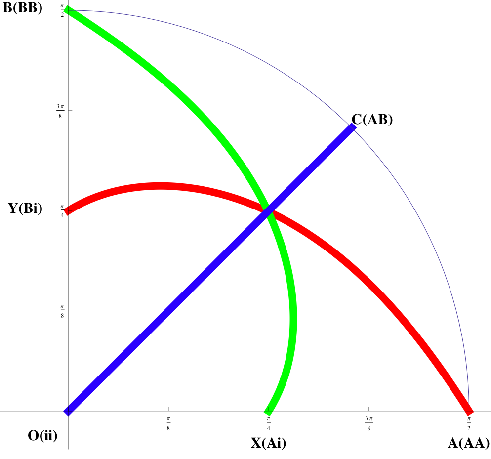
FIG.6. Quadrant with the Blood Type Population Ratio Distribution of World Ethnic Groups from Table 2.
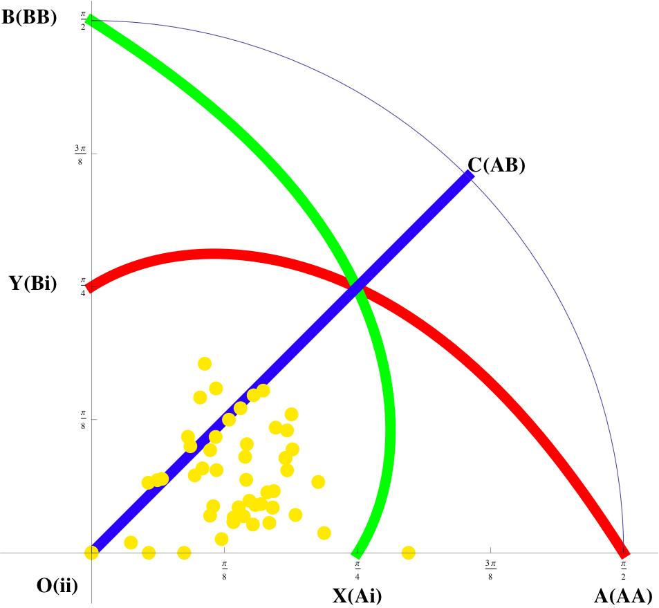
FIG.7. Quadrant with the Blood Type Population Ratio Distribution of World Ethnic Groups from Table 2.
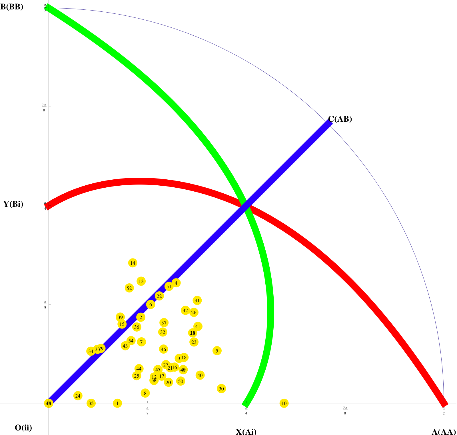
FIG.8. Quadrant with the Blood Type Population Ratio Distribution of World Ethnic Groups from Table 2.
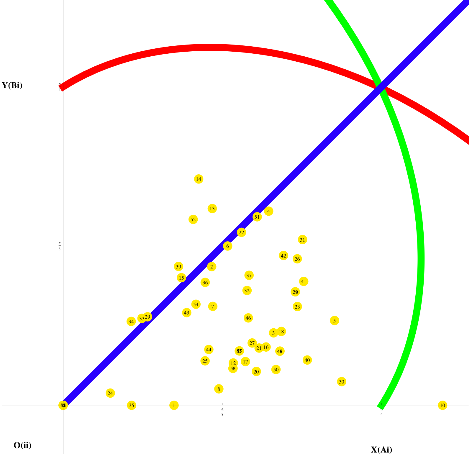
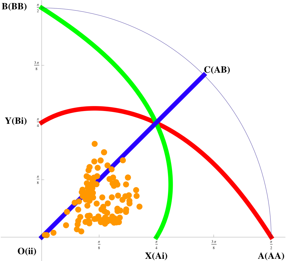
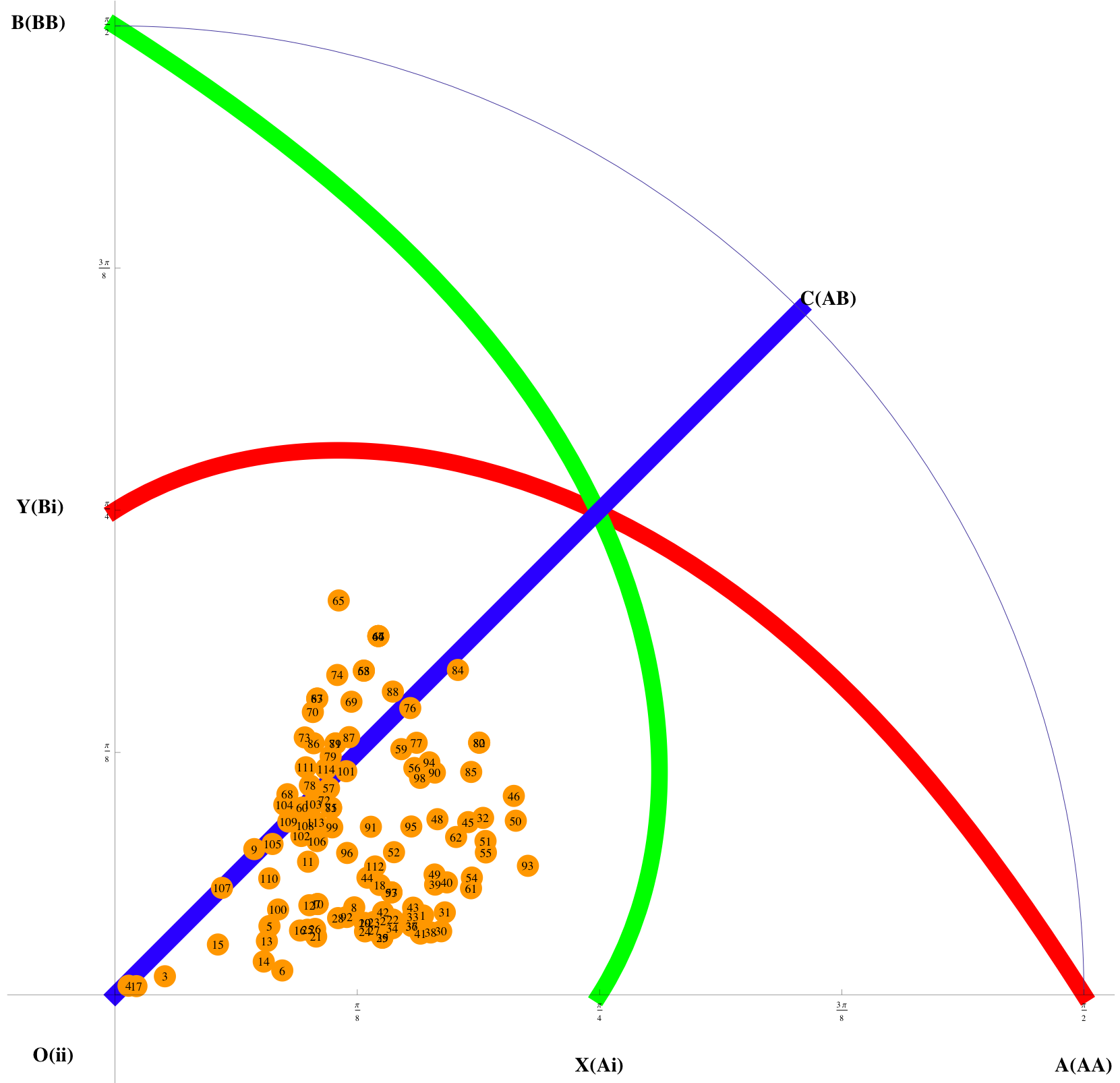
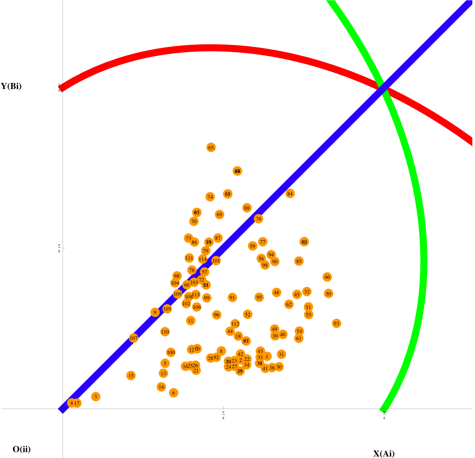
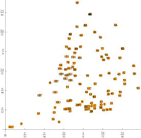
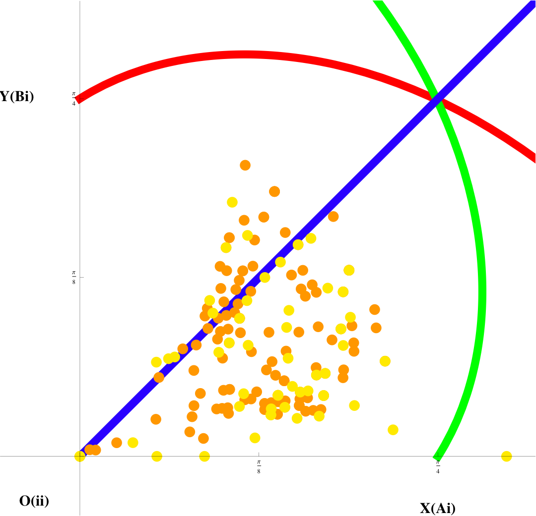
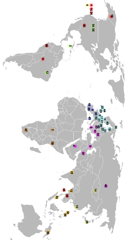
FIG.14. Quadrant with the Blood Type Population Ratio Distribution of World Ethnic Groups from Table 2.
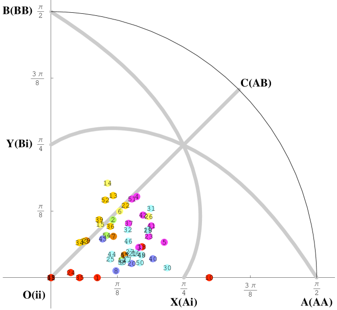
FIG.14. Quadrant with the Blood Type Population Ratio Distribution of World Ethnic Groups from Table 2.
References
- (1) S. Wright, “Systems of mating,” Genetics, 6, 111-178 (1921); “Evolution in Mendelian Populations” Genetics, 16(2): 97-159, (1931); and reference therein.
- (2) R. A. Fisher, “The Genetical Theory of Natural Selection,” Clarendon Press, Oxford (1930).
- (3) J. F. Crow and M. Kimura, “An Introduction to Population Genetics Theory,” Harper and Row, New York (1970)
- (4) Paul Waltman, “Competition Models in Population Biology,” Society for Industrial and Applied Mathematics (1983).
- (5) A. W. F. Edwards, “Foundations of Mathematical Genetics,” 2e, Cambridge University Press (2000).
- (6) W. J. Ewens, “Mathematical Population Genetics,” 2e, Springer (2004).
- (7) G. Mendel, “Versuche über Plflanzenhybriden (Experiments in Plant Hybridization),” Verhandlungen des naturforschenden Vereines in Brünn, Bd. IV für das Jahr 1865, Abhandlungen, 3 47.
- (8) Charles Robert Darwin, “On the Origin of Species,” (1859).
- (9) T. Nagylaki and J. F. Crow, “Continuous selective models,” Theoretical Population Biology 5 257 (1974).
- (10) G. H. Hardy, “Mendelian proportions in a mixed population,” Science 28:49-50 (1908).
- (11) W. Weinberg, “Uber den Nachweis der Vererbung beim Menschen,” Jahreshefte des Verein für vaterländische Naturkunde in Württemberg 64:368-382 (1908).
- (12) http://www.bloodbook.com/world-abo.html http://www.human-abo.org/databank/worldmap.html
- (13) L. L. Cavalli-Sforza and A. W. Edwards, “Phylogenetic analysis: models and estimation procedures,” Evolution 21, 550 (1967).
- (14) M. Nei, “Genetic distance between populations,” The American Naturalist 106, 283 (1972).
- (15) P. L. Antonelli and C. Strobeck, “The geometry of random drift I. Stochastic distance and diffusion,” Advances in Applied Probability 9, 238 (1977).
- (16) P. L. Antonelli and J. Chapin, G. M. Lathrop, and K. Morgan, “The geometry of random drift II. The symmetry of random genetic drift,” Advances in Applied Probability 9, 250 (1977).
- (17) P. L. Antonelli, K. Morgan, and G. M. Lathrop, “The geometry of random drift III. Recombination and diffusion,” Advances in Applied Probability 9, 260 (1977).
- (18) P. L. Antonelli, K. Morgan, and G. M. Lathrop, “The geometry of random drift IV. Random time substitutions and stationary densities,” Advances in Applied Probability 10, 563 (1977).
- (19) J. Reynolds, B. S. Weir, and C. C. Cockerham, “Estimation of the coancestry coefficient: basis for a short-term genetic distance,” Genetics 105, 767 (1983)
- (20) I. DOGAN and N. DOGAN, “Genetic Distance Measures,” Turkiye Klinikleri Journal of Biostatistics 8 (2016).
- (21) For biologists or physicists who are familiar with the renormalization group procedure, the linear stability analysis here is simply finding the relevancy of small perturbations. For any eigenvalue equal to 0, the perturbation is marginal. For any eigenvalue smaller than 0, the perturbation is irrelevant, namely stable against perturbations. For any eigenvalue larger than 0, the perturbation is relevant, namely unstable against perturbations. See, for instance, Mehran Kardar, “Statistical Physics of Fields,” Cambridge University Press (2007), 359 pages.
- (22) Ethan Akin, Joseph M. Szucs, Approaches to the Hardy-Weinberg manifold, Journal of Mathematical Biology, Volume 32, Issue 7, pp 633-643 (1994).
- (23) M.-H. Chung, S. P. Lee, C. K. Kim, and K. Nahm, “Fractional populations of blood groups,” Phys. Rev. E 56, 865 (1997).
- (24) J. Hofbauer and K. Sigmund, “The theory of evolution and dynamical systems,” volume 7 of London Mathematical Society Student Texts. Cambridge University Press, Cambridge. Mathematical aspects of selection, Translated from the German (1988).
- (25) E. Akin and J. M. Szucs, “Approaches to the Hardy-Weinberg manifold.” Journal of Mathematical Biology, 32(7):633-643 (1994).
- (26) J. Jost and J. Pepper, “Individual optimization efforts and population dynamics: a mathematical model for the evolution of resource allocation strategies, with applications to reproductive and mating systems.” Theory in Biosciences, 127(1), pp.31-43 (2008).
- (27) Juven Wang, “Gene-Mating Dynamic Evolution Theory II: Global stability of N-gender-mating polyploid systems.” secondoftwojournal arXiv e-prints , arXiv:1502.07741 (2015), arXiv:1502.07741 [q-bio.PE]
- (28) Juven Wang, et al., “Gene-Mating Dynamic Evolution Theory III: Exactly solvable many-body Boltzmann equation generalization with continuous variables,” in preparation.