Propagation Kernels

Abstract

We introduce propagation kernels, a general graph-kernel framework for efficiently measuring the similarity of structured data. Propagation kernels are based on monitoring how information spreads through a set of given graphs. They leverage early-stage distributions from propagation schemes such as random walks to capture structural information encoded in node labels, attributes, and edge information. This has two benefits. First, off-the-shelf propagation schemes can be used to naturally construct kernels for many graph types, including labeled, partially labeled, unlabeled, directed, and attributed graphs. Second, by leveraging existing efficient and informative propagation schemes, propagation kernels can be considerably faster than state-of-the-art approaches without sacrificing predictive performance. We will also show that if the graphs at hand have a regular structure, for instance when modeling image or video data, one can exploit this regularity to scale the kernel computation to large databases of graphs with thousands of nodes. We support our contributions by exhaustive experiments on a number of real-world graphs from a variety of application domains.

1 Introduction

Learning from structured data is an active area of research. As domains of interest become increasingly diverse and complex, it is important to design flexible and powerful methods for analysis and learning. By structured data we refer to situations where objects of interest are structured and hence can naturally be represented using graphs. Real-world examples are molecules or proteins, image annotated with semantic information, text documents reflecting complex content dependencies, and manifold data modeling objects and scenes in robotics. The goal of learning with graphs is to exploit the rich information contained in graphs representing structured data. The main challenge is to efficiently exploit the graph structure for machine-learning tasks such as classification or retrieval. A popular approach to learning from structured data is to design graph kernels measuring the similarity between graphs. For classification or regression problems, the graph kernel can then be plugged into a kernel machine, such as a support vector machine or a Gaussian process, for efficient learning and prediction.

Several graph kernels have been proposed in the literature, but they often make strong assumptions as to the nature and availability of information related to the graphs at hand. The most simple of these proposals assume that graphs are unlabeled and have no structure beyond that encoded by their edges. However, graphs encountered in real-world applications often come with rich additional information attached to their nodes and edges. This naturally implies many challenges for representation and learning such as:

• missing information leading to partially labeled graphs,

• uncertain information arising from aggregating information from multiple sources, and

• continuous information derived from complex and possibly noisy sensor measurements.

Images, for instance, often have metadata and semantic annotations which are likely to be only partially available due to the high cost of collecting training data. Point clouds captured by laser range sensors consist of continuous 3d coordinates and curvature information; in addition, part detectors can provide possibly noisy semantic annotations. Entities in text documents can be backed by entire Wikipedia articles providing huge amounts of structured information, themselves forming another network.

Surprisingly, existing work on graph kernels does not broadly account for these challenges. Most of the existing graph kernels shervashidzeVPMB09,ShervashidzeB11,HidoK09,KashimaTI03,GartnerFW03 are designed for unlabeled graphs or graphs with a complete set of discrete node labels. Kernels for graphs with continuous node attributes have only recently gained greater interest borgwardtK05,KriegeM12,FeragenKPBB13. These graph kernels have two major drawbacks: they can only handle graphs with complete label or attribute information in a principled manner and they are either efficient, but limited to specific graph types, or they are flexible, but their computation is memory and/or time consuming. To overcome these problems, we introduce propagation kernels. Their design is motivated by the observation that iterative information propagation schemes originally developed for within-network relational and semi-supervised learning have two desirable properties: they capture structural information and they can often adapt to the aforementioned issues of real-world data. In particular, propagation schemes such as diffusion or label propagation can be computed efficiently and they can be initialized with uncertain and partial information.

A high-level overview of the propagation kernel algorithm is as follows. We begin by initializing label and/or attribute distributions for every node in the graphs at hand. We then iteratively propagate this information along edges using an appropriate propagation scheme. By maintaining entire distributions of labels and attributes, we can accommodate uncertain information in a natural way. After each iteration, we compare the similarity of the induced node distributions between each pair of graphs. Structural similarities between graphs will tend to induce similar local distributions during the propagation process, and our kernel will be based on approximate counts of the number of induced similar distributions throughout the information propagation.

To achieve competitive running times and to avoid having to compare the distributions of all pairs of nodes between two given graphs, we will exploit locality sensitive hashing (lsh) to bin the label/attribute distributions into efficiently computable graph feature vectors in time linear in the total number of nodes. These new graph features will then be fed into a base kernel, a common scheme for constructing graph kernels. Whereas lsh is usually used to preserve the $\ell^{1}$ or $\ell^{2}$ distance, we are able to show that the hash values can preserve both the total variation and the Hellinger probability metrics. Exploiting explicit feature computation and efficient information propagation, propagation kernels allow for using graph kernels to tackle novel applications beyond the classical benchmark problems on datasets of chemical compounds and small- to medium-sized image or point-cloud graphs.

Propagation kernels were originally defined and applied for graphs with discrete node labels NeumannPGK12,Neumann13mlg; here we extend their definition to a more general and flexible framework that is able to handle continuous node attributes. In addition to this expanded view of propagation kernels, we also introduce and discuss efficient propagation schemes for numerous classes of graphs. A central message is:

A suitable propagation scheme is the key to designing

fast and powerful propagation kernels.

In particular, we will discuss propagation schemes applicable to huge graphs with regular structure, for example grid graphs representing images or videos. Thus, implemented with care, propagation kernels can easily scale to large image databases. The design of kernels for grids allows us to perform graph-based image analysis not only on the scene level NeumannPGK12,HarchaouiB07 but also on the pixel level opening up novel application domain for graph kernels.

We proceed as follows. We begin by touching upon related work on kernels and graphs. After introducing information propagation on graphs via random walks, we introduce the family of propagation kernels (Section 4). The following two sections discuss specific examples of the two main components of propagation kernels: node kernels for comparing propagated information (Section 5) and propagation schemes for various kinds of information (Section 6). We will then analyze the sensitivity of propagation kernels with respect to noisy and missing information, as well as with respect to the choice of their parameters. Finally, to demonstrate the feasibility and power of propagation kernels for large real-world graph databases, we provide experimental results on several challenging classification problems, including commonly used bioinformatics benchmark problems, as well as real-world applications such as image-based plant-disease classification and 3d object category prediction in the context of robotic grasping.

2 Kernels and Graphs

Propagation kernels are related to three lines of research on kernels: kernels between graphs (graph kernels) developed within the graph mining community, kernels between nodes (kernels on graphs) established in the within-network relational learning and semi-supervised learning communities, and kernels between probability distributions.

2.1 Graph Kernels

Propagation kernels are deeply connected to several graph kernels developed within the graph-mining community. Categorizing graph kernels with respect to how the graph structure is captured, we can distinguish four classes: kernels based on walks GartnerFW03,KashimaTI03,vishwanathanSKB10,HarchaouiB07 and paths borgwardtK05,FeragenKPBB13, kernels based on limited-size subgraphs horvathGW04,shervashidzeVPMB09,KriegeM12, kernels based on subtree patterns maheV09,Ramon03, and kernels based on structure propagation ShervashidzeB11. However, there are two major problems with most existing graph kernels: they are often slow or overly specialized. There are efficient graph kernels specifically designed for unlabeled and fully labeled graphs shervashidzeVPMB09,ShervashidzeB11, attributed graphs FeragenKPBB13, or planar labeled graphs HarchaouiB07, but these are constrained by design. There are also more flexible but slower graph kernels such as the shortest path kernel borgwardtK05 or the common subgraph matching kernel KriegeM12.

The Weisfeiler–Lehman (wl) subtree kernel, one instance of the recently introduced family of wl-kernels ShervashidzeB11, computes count features for each graph based on signatures arising from iterative multi-set label determination and compression steps. In each kernel iteration, these features are then fed into a base kernel. The wl-kernel is finally the sum of those base kernels over the iterations.

Although wl-kernels are usually competitive in terms of performance and runtime, they are designed for fully labeled graphs. The challenge of comparing large, partially labeled graphs – as considered by propagation kernels introduced in the present paper – remains to a large extent unsolved. One proposal for extending a graph kernel to the partially labeled case is to mark unlabeled nodes with a unique symbol, as suggested in ShervashidzeB11. However, collapsing all unlabeled nodes into a single label neglects any notion of uncertainty in the labels. Another option is to propagate labels across the graph and then run a graph kernel on the imputed labels NeumannPGK12. Unfortunately, this also ignores the uncertainty induced by the inference procedure, as hard labels have to be assigned after convergence. A key observation motivating propagation kernels is that intermediate label distributions induced well before convergence carry information about the structure of the graph. Propagation kernels interleave label inference and kernel computation steps, avoiding the requirement of running inference to termination.

2.2 Kernels on Graphs and Within-network Relational Learning

Measuring the structural similarity of local node neighborhoods has recently become popular for inference in networked data KondorL02,Desrosiers09,NeumannGK13 where this idea has been used for designing kernels on graphs (kernels between the nodes of a graph) and for within-network relational learning approaches. An example of the former are coinciding walk kernels NeumannGK13 which are defined in terms of the probability that the labels encountered during parallel random walks starting from the respective nodes of a graph coincide. Desrosiers et al. Desrosiers09 use a similarity measure based on parallel random walks with constant termination probability in a relaxation-labeling algorithm. Another approach exploiting random walks and the structure of subnetworks for node-label prediction is heterogeneous label propagation HwangK10. Random walks with restart are used as proximity weights for so-called “ghost edges” in GallagherGhost08, but then the features considered by a later bag of logistic regression classifiers are only based on a one-step neighborhood. The connection between these approaches and propagation kernels, which is based on the use of random walks to measure structure similarity, constitutes an important contact point of graph-based machine learning for inference about node- and graph-level properties.

2.3 Kernels between Probability Distributions and Kernels between Sets

Finally, propagation kernels mark another contact point, namely between graph kernels and kernels between probability distributions JaakkolaH98,laffertyL02,morenoHV03,jebaraKH04 and between sets KondorJ03,ShiPDLSV09. However, whereas the former essentially build kernels based on the outcome of probabilistic inference after convergence, propagation kernels intuitively count common sub-distributions induced after each iteration of running inference in two graphs.

Kernels between sets and more specifically between structured sets, also called hash kernels ShiPDLSV09, have been successfully applied to strings, data streams, and unlabeled graphs. While propagation kernels hash probability distributions and derive count features from them, hash kernels directly approximate the kernel values $k(x,x^{\prime})$, where $x$ and $x^{\prime}$ are (structured) sets. Propagation kernels iteratively approximate node kernels $k(v_{i},v_{j})$ comparing a node $v_{i}$ in graph $G^{(i)}$ with a node $v_{j}$ in graph $G^{(j)}$. Counts summarizing these approximations are then fed into a base kernel that is computed exactly. Before we give a detailed definition of propagation kernels, we introduce the basic concept of information propagation on graphs, and exemplify important propagation schemes and concepts when utilizing random walks for learning with graphs.

3 Information Propagation on Graphs

Information propagation or diffusion on a graph is most commonly modeled via Markov random walks (rws). Propagation kernels measure the similarity of two graphs by comparing node label or attribute distributions after each step of an appropriate random walk. In the following, we review label diffusion and label propagation via rws – two techniques commonly used for learning on the node level ZhuGL03,SzummerJ01. Based on these ideas, we will then develop propagation kernels in the subsequent sections.

3.1 Basic Notation

Throughout, we consider graphs whose nodes are endowed with (possibly partially observed) label and/or attribute information. That is, a graph $G=(V,E,\ell)$ is represented by a set of $|V|=n$ vertices, a set of edges $E$ specified by a weighted adjacency matrix $A\in\mathbb{R}^{n\times n}$, and a label function $\ell\colon V\rightarrow\mathcal{L}$ with $\mathcal{L}=\left([k],\mathbb{R}^{D}\right)$, where $k$ is the number of available node labels and $D$ is the dimension of the continuous attributes. Given $V=\{v_{1},v_{2},...,v_{n}\}$, node labels $\ell(v_{i})$ are represented by nominal values and attributes $\mathbf{x}_{i}\in\mathbb{R}^{D}$ are represented by continuous vectors.

3.2 Markov Random Walks

Consider a graph $G=(V,E)$. A random walk on $G$ is a Markov process $X=\{X_{t}:t\geq 0\}$ with a given initial state $X_{0}=v_{i}$. We will also write $X_{t}^{(i)}$ to indicate that the walk began at $v_{i}$. The transition probability $T_{ij}=P(X_{t+1}=v_{j}\mid X_{t}=v_{i})$ only depends on the current state $X_{t}=v_{i}$ and the one-step transition probabilities for all nodes in $V$ can be easily represented by the row-normalized adjacency or transition matrix $T=D^{-1}A$, where $D=\operatorname{diag}(\sum_{j}A_{ij})$.

3.3 Information Propagation via Random Walks

For now, we consider (partially) labeled graphs without attributes, where $V=V_{L}\cup V_{U}$ is the union of labeled and unlabeled nodes and $\ell\colon V\rightarrow[k]$ is a label function with known values for the nodes in $V_{L}$. A common mechanism for providing labels for the nodes of an unlabeled graph is to define the label function by $\ell(v_{i})=\sum_{j}A_{ij}=\text{degree}(v_{i})$. Hence for fully labeled and unlabeled graphs we have $V_{U}=\emptyset$. We will monitor the distribution of labels encountered by random walks leaving each node in the graph to endow each node with a $k$-dimensional feature vector. Let the matrix $P_{0}\in\mathbb{R}^{n\times k}$ give the prior label distributions of all nodes in $V.$ If node $v_{i}\in V_{L}$ is observed with label $\ell(v_{i})$, then the $i$th row in $P_{0}$ can be conveniently set to a Kronecker delta distribution concentrating at $\ell(v_{i})$; i.e., $(P_{0})_{i}=\delta_{\ell(v_{i})}$. Thus, on graphs with $V_{U}=\emptyset$ the simplest rw-based information propagation is the label diffusion process or simply diffusion process

$$P_{t+1}\leftarrow TP_{t},$$ (1)

where $(P_{t})_{i}$ gives the distribution over $\ell(X_{t}^{(i)})$ at iteration $t$.

Let $S\subseteq V$ be a set of nodes in $G$. Given $T$ and $S$, we define an absorbing random walk to have the modified transition probabilities $\hat{T}$, defined by:

$$\hat{T}_{ij}=\left\{\begin{array}[]{l l}0&\text{if $i\in S$ and $i\neq j$};\\ 1&\text{if $i\in S$ and $i=j$};\\ T_{ij}&\text{otherwise.}\end{array}\right.$$ (5)

Nodes in $S$ are “absorbing” in that a walk never leaves a node in $S$ after it is encountered. The $i$th row of $P_{0}$ now gives the probability distribution for the first label encountered, $\ell(X_{0}^{(i)})$, for an absorbing rw starting at $v_{i}$. It is easy to see by induction that by iterating the map

$$P_{t+1}\leftarrow\hat{T}P_{t},$$ (6)

$(P_{t})_{i}$ similarly gives the distribution over $\ell(X_{t}^{(i)})$.

In the case of partially labeled graphs we can now initialize the label distributions for the unlabeled nodes $V_{U}$ with some prior, for example a uniform distribution. If we define the absorbing states to be the labeled nodes, $S=V_{L}$, then the label propagation algorithm introduced in ZhuGL03 can be cast in terms of simulating label-absorbing rws with transition probabilities given in Eq. (5) until convergence, then assigning the most probable absorbing label to the nodes in $V_{U}$.

The schemes discussed so far are two extreme cases of absorbing rws: one with no absorbing states, the diffusion process, and one which absorbs at all labeled nodes, label propagation. One useful extension of absorbing rws is to soften the definition of absorbing states. This can be naturally achieved by employing partially absorbing random walks WU12. As the propagation kernel framework does not require a specific propagation scheme, we are free to choose any rw-based information propagation scheme suitable for the given graph types. Based on the basic techniques introduced in this section, we will suggest specific propagation schemes for (un-)labeled, partially labeled, directed, and attributed graphs as well as for graphs with regular structure in Section 6.

3.4 Steady-state Distributions vs. Early Stopping

Assuming non-bipartite graphs, all rws, absorbing or not, converge to a steady-state distribution $P_{\infty}$ Lovasz96,WU12. Most existing rw-based approaches only analyze the walks’ steady-state distributions to make predictions KondorL02,ZhuGL03,WU12. However, rws without absorbing states converge to a constant steady-state distribution, which is clearly uninteresting. To address this, the idea of early stopping was successfully introduced into power-iteration methods for clustering LinC10_PIC, node-label prediction SzummerJ01, as well as for the construction of a kernel for node-label prediction NeumannGK13. The insight here is that the intermediate distributions obtained by the rws during the convergence process provide useful insights about their structure. In this paper, we adopt this idea for the construction of graph kernels. That is, we use the entire evolution of distributions encountered during rws up to a given length to represent graph structure. This is accomplished by summing contributions computed from the intermediate distributions of each iteration, rather then only using the limiting distribution. In the next section, we define the family of propagation kernels.

4 Propagation Kernel Framework

In this section, we introduce the general family of propagation kernels (pks).

4.1 General Definition

Here we will define a kernel $K\colon\mathcal{X}\times\mathcal{X}\to\mathbb{R}$ among graph instances $G^{(i)}\in\mathcal{X}$. The input space $\mathcal{X}$ comprises graphs $G^{(i)}=(V^{(i)},E^{(i)},\ell)$, where $V^{(i)}$ is the set of nodes and $E^{(i)}$ is the set of edges in graph $G^{(i)}$. Edge weights are represented by weighted adjacency matrices $A^{(i)}\in\mathbb{R}^{n_{i}\times n_{i}}$ and the label function $\ell$ endows nodes with label and attribute information as defined in the previous section.

A simple way to compare two graphs $G^{(i)}$ and $G^{(j)}$ is to compare all pairs of nodes in the two graphs:

$$K(G^{(i)},G^{(j)})=\sum_{v\in G^{(i)}}\sum_{u\in G^{(j)}}k(u,v),$$

where $k(u,v)$ is an arbitrary node kernel determined by node labels and, if present, node attributes. This simple graph kernel, however, does not account for graph structure given by the arrangement of node labels and attributes in the graphs. Hence, we consider a sequence of graphs $G^{(i)}_{t}$ with evolving node information based on information propagation, as introduced for node labels in the previous section. We define the kernel contribution of iteration $t$ by

$$K(G^{(i)}_{t},G^{(j)}_{t})=\sum_{v\in G^{(i)}_{t}}\sum_{u\in G^{(j)}_{t}}k(u,v).$$ (7)

An important feature of propagation kernels is that the node kernel $k(u,v)$ is defined in terms of the nodes’ corresponding probability distributions $p_{t,u}$ and $p_{t,v}$, which we update and maintain throughout the process of information propagation. For propagation kernels between labeled and attributed graphs we define

$$k(u,v)=k_{l}(u,v)\cdot k_{a}(u,v),$$ (8)

where $k_{l}(u,v)$ is a kernel corresponding to label information and $k_{a}(u,v)$ is a kernel corresponding to attribute information. If no attributes are present, then $k(u,v)=k_{l}(u,v)$. The $t_{\textsc{max}}$-iteration propagation kernel is now given by

$$K_{t_{\textsc{max}}}(G^{(i)},G^{(j)})=\sum_{t=1}^{t_{\textsc{max}}}K(G^{(i)}_{t},G^{(j)}_{t}).$$ (9)

Lemma 1

Given that $k_{l}(u,v)$ and $k_{a}(u,v)$ are positive semidefinite node kernels, the propagation kernel $K_{t_{\textsc{max}}}$ is a positive semidefinite kernel.

Proof: As $k_{l}(u,v)$ and $k_{a}(u,v)$ are assumed to be valid node kernels, $k(u,v)$ is a valid node kernel as the product of positive semidefinite kernels is again positive semidefinite. As for a given graph $G^{(i)}$ the number of nodes is finite, $K(G^{(i)}_{t},G^{(j)}_{t})$ is a convolution kernel Haussler99. As sums of positive semidefinite matrices are again positive semidefinite, the propagation kernel as defined in Eq. (9) is positive semidefinite.

$\Box$

Algorithm 1 The general propagation kernel computation.

given: graph database $\{G^{(i)}\}_{i}$, $\#$ iterations $t_{\textsc{max}}$, propagation scheme(s), base kernel $\langle\cdot,\cdot\rangle$

$K\leftarrow 0$, $initialize\;\,distributions\;\,P_{0}^{(i)}$

for $t\leftarrow 0\dotsc t_{\textsc{max}}$ do

     for all graphs $G^{(i)}$ do

         for all nodes $u\in G^{(i)}$ do

              $quantize\;\;p_{t,u}$, where $p_{t,u}\text{ is }u\text{-th row in }P^{(i)}_{t}$ $\triangleright$ bin node information

         end for

         $compute\;\;\Phi_{i\cdot}=\phi(G^{(i)}_{t})$ $\triangleright$ count bin strengths

     end for

     $K\leftarrow K+\langle\Phi,\Phi\rangle$ $\triangleright$ compute and add kernel contribution

     for all graphs $G^{(i)}$ do

         $P^{(i)}_{t+1}\leftarrow P^{(i)}_{t}$ $\triangleright$ propagate node information

     end for

end for

(a) Initial label distributions ($t=0$)

(b) Updated label distributions ($t=1$)

Figure 1: Propagation Kernel Computation. Distributions, bins, count features, and kernel contributions for two graphs $G^{(i)}$ and $G^{(j)}$ with binary node labels and one iteration of label propagation, cf. Eq. (6), as the propagation scheme. Node-label distributions are decoded by color: white means $p_{0,u}=[1,0]$, dark red stands for $p_{0,u}=[0,1]$, and the initial distributions for unlabeled nodes (light red) are $p_{0,u}=[\nicefrac{{1}}{{2}},\nicefrac{{1}}{{2}}]$.

Let $|V^{(i)}|=n_{i}$ and $|V^{(j)}|=n_{j}$. Assuming that all node information is given, the complexity of computing each contribution between two graphs, Eq. (7), is $\mathcal{O}(n_{i}\,n_{j})$. Even for medium-sized graphs this can be prohibitively expensive considering that the computation has to be performed for every pair of graphs in a possibly large graph database. However, if we have a node kernel of the form

$$k(u,v)=\left\{\begin{array}[]{l l}1&\text{if }condition\\ 0&\text{otherwise},\end{array}\right.$$ (12)

where $condition$ is an equality condition on the information of nodes $u$ and $v$, we can compute $K$ efficiently by binning the node information, counting the respective bin strengths for all graphs, and computing a base kernel among these counts. That is, we compute count features $\phi(G^{(i)}_{t})$ for each graph and plug them into a base kernel: $\langle\cdot,\cdot\rangle$

$$K(G^{(i)}_{t},G^{(j)}_{t})=\langle\phi(G^{(i)}_{t}),\phi(G^{(j)}_{t})\rangle.$$ (13)

In the simple case of a linear base kernel, the last step is just an outer product of count vectors $\Phi_{t}\Phi_{t}^{\top}$, where the $i$th row of $\Phi_{t}$, $\left(\Phi_{t}\right)_{i\,\cdot}=\phi(G^{(i)}_{t})$. Now, for two graphs, binning and counting can be done in $\mathcal{O}(n_{i}+n_{j})$ and the computation of the linear base kernel value is $\mathcal{O}(|\text{bins}|)$. This is a commonly exploited insight for efficient graph-kernel computation and it has already been exploited for labeled graphs in previous work ShervashidzeB11,NeumannPGK12.

Figure 1 illustrates the propagation kernel computation for $t=0$ and $t=1$ for two example graphs and Algorithm 1 summarizes the kernel computation for a graph database $\mathbf{G}=\{G^{(i)}\}_{i}=(V,E,\ell)$ with a total number of $N$ nodes. From this general algorithm and Eqs. (7) and (9), we see that the two main components to design a propagation kernel are

• the node kernel $k(u,v)$ comparing propagated information, and

• the propagation scheme $P^{(i)}_{t+1}\leftarrow P^{(i)}_{t}$ propagating the information within the graphs.

The propagation scheme depends on the input graphs and we will give specific suggestions for different graph types in Section 6. Before defining the node kernels depending on the available node information in Section 5, we briefly discuss the general runtime complexity of propagation kernels.

4.2 Complexity Analysis

The total runtime complexity of propagation kernels for a set of $n$ graphs with a total number of $N$ nodes and $M$ edges is $\mathcal{O}\bigl{(}(t_{\textsc{max}}-1)M+t_{\textsc{max}}\,n^{2}\,n^{\star}\bigr{)}$, where $n^{\star}:=\max_{i}(n_{i})$. For a pair of graphs the runtime complexity of computing the count features, that is, binning the node information and counting the bin strengths is $\mathcal{O}(n_{i}+n_{j})$. Computing and adding the kernel contribution is $\mathcal{O}(|\text{bins}|)$, where $|\text{bins}|$ is bounded by $n_{i}+n_{j}$. So, one iteration of the kernel computation for all graphs is $\mathcal{O}(n^{2}\,n^{\star})$. Note that in practice $|\text{bins}|\ll 2n^{\star}$ as we aim to bin together similar nodes to derive a meaningful feature representation.

Feature computation basically depends on propagating node information along the edges of all graphs. This operation depends on the number of edges and the information propagated, so it is $\mathcal{O}((k+D)M)=\mathcal{O}(M)$, where $k$ is the number of node labels and $D$ is the attribute dimensionality. This operation has to be performed $t_{\textsc{max}}-1$ times. Note that the number of edges is usually much lower than $N^{2}$.

5 Propagation Kernel Component 1: Node Kernel

In this section, we define node kernels comparing label distributions and attribute information appropriate for the use in propagation kernels. Moreover, we introduce locality sensitive hashing, which is used to discretize the distributions arsing from rw-based information propagation and the continuous attribute vectors directly.

5.1 Definitions

Above, we saw that one way to allow for efficient computation of propagation kernels is to restrict the range of the node kernels to $\{0,1\}$. Let us now define the two components of the node kernel (Eq. (8)) in this form. The label kernel can be represented as

$$k_{l}(u,v)=\left\{\begin{array}[]{l l}1&\text{if }h_{l}(p_{t,u})=h_{l}(p_{t,v});\\ 0&\text{otherwise,}\end{array}\right.$$ (16)

where $p_{t,u}$ is the node-label distribution of node $u$ at iteration $t$ and $h_{l}(\cdot)$ is a quantization function Gersho1991, more precisely a locality sensitive hash (lsh) function pstable, which will be introduced in more detail in the next section. Note that $p_{t,u}$ denotes a row in the label distribution matrix $P^{(i)}_{t}$, namely the row corresponding to node $u$ of graph $G^{(i)}$.

Propagation kernels can be computed for various kinds of attribute kernels as long as they have the form of Eq. (12). The most rudimentary attribute kernel is

$$k_{a}(u,v)=\left\{\begin{array}[]{l l}1&\text{if }h_{a}(x_{u})=h_{a}(x_{v})\\ 0&\text{otherwise},\end{array}\right.$$ (19)

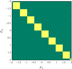
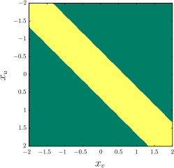
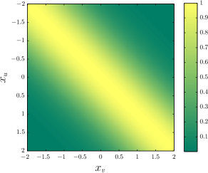
where $x_{u}$ is the one-dimensional continuous attribute of node $u$ and $h_{a}(\cdot)$ is again an lsh function. Figure 2 contrasts this simple attribute kernel for a one-dimensional attribute to a thresholded Gaussian function and the Gaussian kernel commonly used to compare node attributes in graph kernels. To deal with higher-dimensional attributes, we can choose the attribute kernel to be the product of kernels on each attribute dimension:

$$k_{a}(u,v)=\prod_{d=1}^{D}k_{a_{d}}(u,v),\text{ where}$$

$$k_{a_{d}}(u,v)=\left\{\begin{array}[]{l l}1&\text{if }h_{a_{d}}(x^{(d)}_{u})=h_{a_{d}}(x^{(d)}_{v});\\ 0&\text{otherwise},\end{array}\right.$$ (22)

where $x^{(d)}_{u}$ is the respective dimension of the attribute $\mathbf{x}_{u}$ of node $u$. Note that each dimension now has its own lsh function $h_{a_{d}}(\cdot)$. However, analogous to the label kernel, we can also define an attribute kernel based on propagated attribute distributions

$$k_{a}(u,v)=\left\{\begin{array}[]{l l}1&\text{if }h_{a}(q_{t,u})=h_{a}(q_{t,v})\\ 0&\text{otherwise},\end{array}\right.$$ (25)

where $q_{t,u}$ is the attribute distribution of node $u$ at iteration $t$. Next we explain the locality sensitive hashing approach used to discretize distributions and continuous attributes. In Section 6.3, we will then derive an efficient way to propagate and hash continuous attribute distributions.

(a) $k_{a}(u,v)$

(b) thresholded Gaussian

(c) Gaussian kernel

Figure 2: Attribute Kernels. Three different attribute functions among nodes with continuous attributes $x_{u}$ and $x_{v}\in\left[-2,2\right]$. Panel (a) illustrates an attribute kernel suitable for the efficient computation in propagation kernels, Panel (b) shows a thresholded Gaussian, and Panel (c) a Gaussian kernel.

5.2 Locality Sensitive Hashing

We now describe our quantization approach for implementing propagation kernels for graphs with node-label distributions and continuous attributes. The idea is inspired by locality-sensitive hashing pstable which seeks quantization functions on metric spaces where points “close enough” to each other in that space are “probably” assigned to the same bin. In the case of distributions, we will consider each node-label vector as being an element of the space of discrete probability distributions on $k$ items equipped with an appropriate probability metric. If we want to hash attributes directly, we simply consider metrics for continuous values.

Definition 1 (Locality Sensitive Hash (lsh))

Let $\mathcal{X}$ be a metric space with metric $d\colon\mathcal{X}\times\mathcal{X}\to\mathbb{R}$, and let $\mathcal{Y}=\{1,2,\dotsc,k^{\prime}\}$. Let $\theta>0$ be a threshold, $c>1$ be an approximation factor, and $p_{1},p_{2}\in(0,1)$ be the given success probabilities. A set of functions $\mathcal{H}$ from $\mathcal{X}$ to $\mathcal{Y}$ is called a $(\theta,c\theta,p_{1},p_{2})$-locality sensitive hash if for any function $h\in\mathcal{H}$ chosen uniformly at random, and for any two points $x,x^{\prime}\in\mathcal{X}$, it holds that
  $-$ if $d(x,x^{\prime})<\phantom{c}\theta$, then $\Pr(h(x)=h(x^{\prime}))>p_{1}$, and
  $-$ if $d(x,x^{\prime})>c\theta$, then $\Pr(h(x)=h(x^{\prime}))<p_{2}$.

It is known that we can construct lsh families for $\ell^{p}$ spaces with $p\in(0,2]$ pstable. Let $V$ be a real-valued random variable. $V$ is called $p$-stable if for any $\{x_{1},x_{2},$ $\dotsc,x_{d}\}$, $x_{i}\in\mathbb{R}$ and independently sampled $v_{1},v_{2},\dotsc,v_{d}$, we have $\sum x_{i}v_{i}\sim\lVert\mathbf{x}\rVert_{p}V$. Explicit $p$-stable distributions are known for some $p$; for example, the standard Cauchy distribution is 1-stable, and the standard normal distribution is 2-stable. Given the ability to sample from a $p$-stable distribution $V$, we may define an lsh $\mathcal{H}$ on $\mathbb{R}^{d}$ with the $\ell^{p}$ metric pstable. An element $h$ of $\mathcal{H}$ is specified by three parameters: a width $w\in\mathbb{R}^{+}$, a $d$-dimensional vector $\mathbf{v}$ whose entries are independent samples of $V$, and $b$ drawn from $\mathcal{U}[0,w]$. Given these, $h$ is then defined as

$$h(\mathbf{x};w,\mathbf{v},b)=\left\lfloor\frac{\mathbf{v}^{\top}\mathbf{x}+b}{w}\right\rfloor.$$ (26)

We may now consider $h(\cdot)$ to be a function mapping our distributions or attribute values to integer-valued bins, where similar distributions end up in the same bin. Hence, we obtain node kernels as defined in Eqs. (16) and (25) in the case of distributions, as well as simple attribute kernels as defined in Eqs. (19) and (22). To decrease the probability of collision, it is common to choose more than one random vector $\mathbf{v}$. For propagation kernels, however, we only use one hyperplane, as we effectively have $t_{\textsc{max}}$ hyperplanes for the whole kernel computation and the probability of a hash conflict is reduced over the iterations.

Algorithm 2 calculate-lsh

given: matrix $X\in\mathbb{R}^{N\times D}$, bin width $w$, metric m

if m = h then

     $X\leftarrow\sqrt{X}$ $\triangleright$ square root transformation

end if

if m = h or m = l2 then $\triangleright$ generate random projection vector

     $v\leftarrow\textsc{rand-norm}(D)$ $\triangleright$ sample from $\mathcal{N}(0,1)$

else if  m = tv or m = l1 then

     $v\leftarrow\textsc{rand-norm}(D)/\textsc{rand-norm}(D)$ $\triangleright$ sample from $\mathcal{C}auchy(0,1)$

end if

$b=w*\text{{rand-unif()}}$ $\triangleright$ random offset $b\sim\mathcal{U}\left[0,w\right]$

$h(X)=\text{floor}((X*v+b)/w)$ $\triangleright$ compute hashes

The intuition behind the expression in Eq. (26) is that $p$-stability implies that two vectors that are close under the $\ell^{p}$ norm will be close after taking the dot product with $\mathbf{v}$; specifically, $(\mathbf{v}^{\top}\mathbf{x}-\mathbf{v}^{\top}\mathbf{x^{\prime}})$ is distributed as $\lVert\mathbf{x}-\mathbf{x}^{\prime}\rVert_{p}V$. So, in the case where we want to construct a hashing for $D$-dimensional continuous node attributes to preserve $\ell^{1}$ (l1) or $\ell^{2}$ (l2) distance

$$d_{\text{{l1}}}(x_{u},x_{v})=\sum^{D}_{d=1}\,\lvert x^{(d)}_{u}-x^{(d)}_{v}\rvert,\;\;\;d_{\text{{l2}}}(x_{u},x_{v})=\left(\sum^{D}_{d=1}\,\bigl{(}x^{(d)}_{u}-x^{(d)}_{v}\bigr{)}^{2}\right)^{\nicefrac{{1}}{{2}}}\!\!\!\!,$$

we directly apply Eq. (26). In the case of distributions, we are concerned with the space of discrete probability distributions on $k$ elements, endowed with a probability metric $d$. Here we specifically consider the total variation (tv) and Hellinger (h) distances:

$$d_{\text{{tv}}}(p_{u},p_{v})=\nicefrac{{1}}{{2}}\sum^{k}_{i=1}\,\lvert p^{(i)}_{u}-p^{(i)}_{v}\rvert,\;\;\;d_{\text{{h}}}(p_{u},p_{v})=\left(\nicefrac{{1}}{{2}}\sum^{k}_{i=1}\,\bigl{(}\sqrt{p^{(i)}_{u}}-\sqrt{p^{(i)}_{v}}\bigr{)}^{2}\right)^{\nicefrac{{1}}{{2}}}\!\!\!\!.$$

The total variation distance is simply half the $\ell^{1}$ metric, and the Hellinger distance is a scaled version of the $\ell^{2}$ metric after applying the map $p\mapsto\sqrt{p}$. We may therefore create a locality-sensitive hash family for $d_{\text{{tv}}}$ by direct application of Eq. (26) and create a locality-sensitive hash family for $d_{\text{{h}}}$ by using Eq. (26) after applying the square root map to our label distributions. The lsh computation for a matrix $X\in\mathbb{R}^{N\times D}$, where the $u$-th row of $X$ is $\mathbf{x}_{u}$, is summarized in Algorithm 2.

6 Propagation Kernel Component 2: Propagation Scheme

As pointed out in the introduction, the input graphs for graph kernels may vary considerably. One key insight to the design of efficient and powerful propagation kernels is to choose an appropriate propagation scheme for the graph dataset at hand. By utilizing random walks (rws) we are able to use efficient off-the-shelf algorithms, such as label diffusion or label propagation SzummerJ01,ZhuGL03,WU12, to implement information propagation on the input graphs. In this section, we explicitly define propagation kernels appropriate for fully labeled, unlabeled, partially labeled, directed, and attributed graphs as well as for graphs with a regular grid structure. In each particular algorithm, the specific parts changing compared to the general propagation kernel computation (Algorithm 1) will be marked in color.

6.1 Labeled and Unlabeled Graphs

For fully labeled graphs we suggest the use of the label diffusion process from Eq. (1) as the propagation scheme. Given a database of fully labeled graphs $\mathbf{G}=\{G^{(i)}\}_{i=1,\dots,n}$ with a total number of $N=\sum_{i}n_{i}$ nodes, label diffusion on all graphs can be efficiently implemented by multiplying a sparse block-diagonal transition matrix $T\in\mathbb{R}^{N\times N}$, where the blocks are the transition matrices $T^{(i)}$ of the respective graphs, with the label distribution matrix $P_{t}=\left[P^{(1)}_{t},\dots,P^{(n)}_{t}\right]^{\top}\in\mathbb{R}^{N\times k}$. This can be done efficiently due to the sparsity of $T$. The propagation kernel computation for labeled graphs is summarized in Algorithm 3. The specific parts compared to the general propagation kernel computation (Algorithm 1) for fully labeled graphs are marked in green (input) and blue (computation). For unlabeled graphs we suggest to set the label function to be the node degree $\ell(u)=\text{degree}(u)$ and then apply the same pk computation as for fully labeled graphs.

Algorithm 3 Propagation kernel for fully labeled graphs.

given: graph database $G=(V,E,\ell)$, $\#$ iterations $t_{\textsc{max}}$, transition matrix $\color[rgb]{0,0.88,0}\definecolor[named]{pgfstrokecolor}{rgb}{0,0.88,0}\pgfsys@color@cmyk@stroke{0.91}{0}{0.88}{0.12}\pgfsys@color@cmyk@fill{0.91}{0}{0.88}{0.12}T$, bin width $w$, metric m, base kernel $\langle\cdot,\cdot\rangle$

initialization: $K\leftarrow 0$, $\color[rgb]{0,0,1}\definecolor[named]{pgfstrokecolor}{rgb}{0,0,1}P_{0}\leftarrow\delta_{\ell(V)}$

for $t\leftarrow 0\dotsc t_{\textsc{max}}$ do

     calculate-lsh($P_{t}$, $w$, m) $\triangleright$ bin node information

     for all graphs $G^{(i)}$ do

         $compute\;\;\Phi_{i\cdot}=\phi(G^{(i)}_{t})$ $\triangleright$ count bin strengths

     end for

     $\color[rgb]{0,0,1}\definecolor[named]{pgfstrokecolor}{rgb}{0,0,1}P_{t+1}\leftarrow TP_{t}$ $\triangleright$ label diffusion

     $K\leftarrow K+\langle\Phi,\Phi\rangle$ $\triangleright$ compute and add kernel contribution

end for

6.2 Partially Labeled and Directed Graphs

For partially labeled graphs, where some of the node labels are unknown, we suggest label propagation as an appropriate propagation scheme. Label propagation differs from label diffusion in the fact that before each iteration of the information propagation, the labels of the originally labeled nodes are pushed back ZhuGL03. Let $P_{0}=\left[P_{0,[\text{labeled}]},P_{0,[\text{unlabeled}]}\right]^{\top}$ represent the prior label distributions for the nodes of all graphs in a graph database $\mathbf{G}=(V,E,\ell)$, where the distributions in $P_{0,[\text{labeled}]}$ represent observed labels and $P_{0,[\text{unlabeled}]}$ are initialized uniformly. Then label propagation is defined by

$$P_{t,[labeled]} \leftarrow P_{0,[\text{labeled}]};$$

$$P_{t+1} \leftarrow T\,P_{t}.$$ (27)

Note that this propagation scheme is equivalent to the one defined in Eq. (6) using partially absorbing rws. Other similar update schemes, such as “label spreading” ZhouBLWS03, could be used in a propagation kernel as well. Thus, the propagation kernel computation for partially labeled graphs is essentially the same as Algorithm 3, where the initialization for the unlabeled nodes has to be adapted, and the (partial) label push back has to be added before the node information is propagated. The relevant parts are the ones marked in blue. Note that for graphs with large fractions of labeled nodes it might be preferable to use label diffusion even though they are partially labeled.

To implement propagation kernels between directed graphs, we can proceed as above after simply deriving transition matrices computed from the potentially non-symmetric adjacency matrices. That is, for the propagation kernel computation only the input changes (marked in green in Algorithm 3). The same idea allows weighted edges to be accommodated; again, only the transition matrix has to be adapted. Obviously, we can also combine partially labeled graphs with directed or weighted edges by changing both the blue and green marked parts accordingly.

6.3 Graphs with Continuous Node Attributes

Nowadays, learning tasks often involve graphs whose nodes are attributed with continuous information. Chemical compounds can be annotated with the length of the secondary structure elements (the nodes) or measurements for various properties, such as hydrophobicity or polarity. 3d point clouds can be enriched with curvature information, and images are inherently composed of 3-channel color information. All this information can be modeled by continuous node attributes. In Eq. (19) we introduced a simple way to deal with attributes. The resulting propagation kernel essentially counts similar label arrangements only if the corresponding node attributes are similar as well. Note that for higher-dimensional attributes it can be advantageous to compute separate lshs per dimension, leading to the node kernel introduced in Eq. (22). This has the advantage that if we standardize the attributes, we can use the same bin-width parameter $w_{a}$ for all dimensions. In all our experiments we normalize each attribute to have unit standard deviation and will set $w_{a}=1$. The disadvantage of this method, however, is that the arrangement of attributes in the graphs is ignored.

Algorithm 4 Propagation kernel (p2k) for attributed graphs.

given: graph database $G=(V,E,\ell)$, $\#$ iterations $t_{\textsc{max}}$, transition matrix $\color[rgb]{0,0.88,0}\definecolor[named]{pgfstrokecolor}{rgb}{0,0.88,0}\pgfsys@color@cmyk@stroke{0.91}{0}{0.88}{0.12}\pgfsys@color@cmyk@fill{0.91}{0}{0.88}{0.12}T$, bin widths $w_{l}$, $w_{a}$, metrics m_l, m_a, base kernel $\langle\cdot,\cdot\rangle$

initialization: $K\leftarrow 0$, $P_{0}\leftarrow\delta_{\ell(V)}$

$\color[rgb]{0,0,1}\definecolor[named]{pgfstrokecolor}{rgb}{0,0,1}\boldsymbol{\mu}=X$, $\color[rgb]{0,0,1}\definecolor[named]{pgfstrokecolor}{rgb}{0,0,1}\Sigma=\operatorname{cov}(X)$, $\color[rgb]{0,0,1}\definecolor[named]{pgfstrokecolor}{rgb}{0,0,1}W_{0}=I$ $\triangleright$ gm initialization

$\color[rgb]{0,0,1}\definecolor[named]{pgfstrokecolor}{rgb}{0,0,1}y\leftarrow\text{{rand}}(\text{num-samples})$ $\triangleright$ sample points for gm evaluations

for $t\leftarrow 0\dotsc t_{\textsc{max}}$ do

     $h_{l}\leftarrow$ calculate-lsh($P_{t}$, $w_{l}$, m_l) $\triangleright$ bin label distributions

     $\color[rgb]{0,0,1}\definecolor[named]{pgfstrokecolor}{rgb}{0,0,1}Q_{t}\leftarrow$ evaluate-pdfs($\boldsymbol{\mu}$, $\Sigma$, $W_{t}$, $y$) $\triangleright$ evaluate gms at $y$

     $\color[rgb]{0,0,1}\definecolor[named]{pgfstrokecolor}{rgb}{0,0,1}h_{a}\leftarrow$ calculate-lsh($Q_{t}$, $w_{a}$, m_a) $\triangleright$ bin attribute distributions

     $\color[rgb]{0,0,1}\definecolor[named]{pgfstrokecolor}{rgb}{0,0,1}h\leftarrow h_{l}\wedge h_{a}$ $\triangleright$ combine label and attribute bins

     for all graphs $G^{(i)}$ do

         $compute\;\;\Phi_{i\cdot}=\phi(G^{(i)}_{t})$ $\triangleright$ count bin strengths

     end for

     $P_{t+1}\leftarrow TP_{t}$ $\triangleright$ propagate label information

     $\color[rgb]{0,0,1}\definecolor[named]{pgfstrokecolor}{rgb}{0,0,1}W_{t+1}\leftarrow TW_{t}$ $\triangleright$ propagate attribute information

     $K\leftarrow K+\langle\Phi,\Phi\rangle$ $\triangleright$ compute and add kernel contribution

end for

In the following, we derive p2k, a variant of propagation kernels for attributed graphs based on the idea of propagating both attributes and labels. That is, we model graph similarity by comparing the arrangement of labels and the arrangement of attributes in the graph. The attribute kernel for p2k is defined as in Eq. (25); now the question is how to efficiently propagate the continuous attributes and how to efficiently model and hash the distributions of (multivariate) continuous variables. Let $X\in\mathbb{R}^{N\times D}$ be the design matrix, where the $u$th row in $X$ is the attribute vector of node $u$, $\mathbf{x}_{u}$. We will associate with each node of each graph a probability distribution defined on the attribute space, $q_{u}$, and will update these as attribute information is propagated across graph edges as before. One challenge in doing so is ensuring that these distributions can be represented with a finite description. The discrete label distributions from before were naturally finite dimensional and could be compactly represented and updated via the $P_{t}$ matrices. We seek a similar representation for attributes. Our proposal is to define the node-attribute distributions to be mixtures of $D$-dimensional multivariate Gaussians, one centered on each attribute vector in $X$:

$$q_{u}=\sum_{v}W_{uv}\,\mathcal{N}(\mathbf{x}_{v},\Sigma),$$

where the sum ranges over all nodes $v$, $W_{u,\cdot}$ is a vector of mixture weights, and $\Sigma$ is a shared $D\times D$ covariance matrix for each component of the mixture. In particular, here we set $\Sigma$ to be the sample covariance matrix calculated from the $N$ vectors in $X$. Now the $N\times N$ row-normalized $W$ matrix can be used to compactly represent the entire set of attribute distributions. As before, we will use the graph structure to iteratively spread attribute information, updating these $W$ matrices, deriving a sequence of attribute distributions for each node to use as inputs to node attribute kernels in a propagation kernel scheme.

We begin by defining the initial weight matrix $W_{0}$ to be the identity matrix; this is equivalent to beginning with each node attribute distribution being a single Gaussian centered on the corresponding attribute vector:

$$W_{0} =I;$$

$$q_{0,u} =\mathcal{N}(\mathbf{x}_{u},\Sigma).$$

Now, in each propagation step the attribute distributions are updated by the distribution of their neighboring nodes $Q_{t+1}\leftarrow Q_{t}$. We accomplish this by propagating the mixture weights $W$ across the edges of the graph according to a row-normalized transition matrix $T$, derived as before:

$$W_{t+1} \leftarrow TW_{t}=T^{t};$$

$$q_{t+1,u} =\sum_{v}\left(W_{t}\right)_{uv}\,\mathcal{N}(\mathbf{x}_{v},\Sigma).$$ (28)

We have described how we associate attribute distributions with each node and how we update them via propagating their weights across the edges of the graph. However, the weight vectors contained in $W$ are not themselves directly suitable for comparing in an attribute kernel $k_{a}$, because any information about the similarity of the mean vectors is ignored. For example, imagine that two nodes $u$ and $v$ had exactly the same attribute vector, $\mathbf{x}_{u}=\mathbf{x}_{v}$. Then mass on the $u$ component of the Gaussian mixture is exchangeable with mass on the $v$ component, but typical vectorial kernels cannot capture this. For this reason, we use our Gaussian mixtures to associate a vector more appropriate for kernel comparison with each node. Namely, we select a fixed set of sample points in attribute space (in our case, chosen uniformly from the node attribute vectors in $X$), evaluate the pdfs associated with each node at these points, and use this vector to summarize the nodes. This handles the exchangeability issue from above and also allows a more compact representation for hash inputs; in our experiments, we used 100 sample points and achieved good performance. As before, these vectors can then be hashed jointly or individually for each sample point. Note that the bin width $w_{a}$ has to be adapted accordingly. In our experiments, we will use the latter option and set $w_{a}=1$ for all datasets. The computational details of p2k are given in Algorithm 4, where the additional parts compared to Algorithm 1 are marked in blue (computation) and green (input). An extension to Algorithm 4 would be to refit the gms after a couple of propagation iterations. We did not consider refitting in our experiments as the number of kernel iterations $t_{\textsc{max}}$ was set to $10$ or $15$ for all datasets – following the descriptions in existing work on iterative graph kernels ShervashidzeB11,NeumannPGK12.

6.4 Grid Graphs

One of our goals in this paper is to compute propagation kernels for pixel grid graphs. A graph kernel among grid graphs can be defined such that two grids should have a high kernel value if they have similarly arranged node information. This can be naturally captured by propagation kernels as they monitor information spread on the grids. Naïvely, one could think that we can simply apply Algorithm 3 to achieve this goal. However, given that the space complexity of this algorithm scales with the number of edges and even medium sized images such as texture patches will easily contain thousands of nodes, this is not feasible. For example considering $100\times 100$-pixel image patches with an 8-neighborhood graph structure, the space complexity required would be $2.4$ million units (floating point numbers) per graph. Fortunately, we can exploit the flexibility of propagation kernels by exchanging the propagation scheme. Rather than label diffusion as used earlier, we employ discrete convolution; this idea was introduced for efficient clustering on discrete lattices in BauckhageK13. In fact, isotropic diffusion for denoising or sharpening is a highly developed technique in image processing Jahne05. In each iteration, the diffused image is derived as the convolution of the previous image and an isotropic (linear and space-invariant) filter. In the following, we derive a space- and time-efficient way of computing propagation kernels for grid graphs by means of convolutions.

Basic Definitions

Given that the neighborhood of a node is the subgraph induced by all its adjacent vertices, we define a $d$-dimensional grid graph as a lattice graph whose node embedding in $\mathbb{R}^{d}$ forms a regular square tiling and the neighborhoods $\mathcal{N}$ of each non-border node are isomorphic (ignoring the node information). Figure 3 illustrates a regular square tiling and several isomorphic neighborhoods of a $2$-dimensional grid graph. If we ignore boundary nodes, a grid graph is a regular graph; i.e., each non-border node has the same degree. Note that the size of the border depends on the radius of the neighborhood. In order to be able to neglect the special treatment for border nodes, it is common to view the actual grid graph as a finite section of an actually infinite graph.

A grid graph whose node embedding in $\mathbb{R}^{d}$ forms a regular square tiling can be derived from the graph Cartesian product of line graphs. So, a two-dimensional grid is defined as

$$G^{(i)}=L_{m_{i,1}}\times L_{m_{i,2}},$$

where $L_{m_{i,1}}$ is a line graph with $m_{i,1}$ nodes. $G^{(i)}$ consists of $n_{i}=m_{i,1}\,m_{i,2}$ nodes, where non-border nodes have the same number of neighbors. Note that the grid graph $G^{(i)}$ only specifies the node layout in the graph but not the edge structure. The edges are given by the neighborhood $\mathcal{N}$ which can be defined by any arbitrary matrix $B$ encoding the weighted adjacency of its center node. The nodes, being for instance image pixels, can carry discrete or continuous vector-valued information. Thus, in the most-general setting the database of grid graphs is given by $\mathbf{G}=\{G^{(i)}\}_{i=1,\ldots,n}$ with $G^{(i)}=(V^{(i)},\mathcal{N},\ell)$, where $\ell:V^{(i)}\rightarrow\mathcal{L}$ with $\mathcal{L}=([k],\mathbb{R}^{D})$. Commonly used neighborhoods $\mathcal{N}$ are the 4-neighborhood and the $8$-neighborhood illustrated in Figure 3(b) and (c).

(a) Square tiling

(b) $4$-neighborhood

(c) $8$-neighborhood

(d) non-symmetric, neighborhood

Figure 3: Grid Graph. Regular square tiling (a) and three example neighborhoods (b–d) for a $2$-dimensional grid graph derived from line graphs $L_{7}$ and $L_{6}$.

Discrete Convolution

The general convolution operation on two functions $f$ and $g$ is defined as

$$f(x)\ast g(x)=(f\ast g)(x)=\int_{-\infty}^{\infty}f(\tau)\,g(x-\tau)\,\mathrm{d}\tau.$$

That is, the convolution operation produces a modified, or filtered, version of the original function $f$. The function $g$ is called a filter. For two-dimensional grid graphs interpreted as discrete functions of two variables $x$ and $y$, e.g., the pixel location, we consider the discrete spatial convolution defined by:

$$f(x,y)\ast g(x,y)=(f\ast g)(x,y)=\sum_{i=-\infty}^{\infty}\sum_{j=-\infty}^{\infty}f(i,j)\,g(x-i,y-j),$$

where the computation is in fact done for finite intervals. As convolution is a well-studied operation in low-level signal processing and discrete convolution is a standard operation in digital image processing, we can resort to highly developed algorithms for its computation; see for example Chapter 2 in Jahne05. Convolutions can be computed efficiently via the fast Fourier transformation in $\mathcal{O}(n_{i}\,\log\,n_{i})$ per graph.

Algorithm 5 Propagation kernel for grid graphs.

given: graph database $G=(V,E,\ell)$, $\#$ iterations $t_{\textsc{max}}$, filter matrix $\color[rgb]{0,0.88,0}\definecolor[named]{pgfstrokecolor}{rgb}{0,0.88,0}\pgfsys@color@cmyk@stroke{0.91}{0}{0.88}{0.12}\pgfsys@color@cmyk@fill{0.91}{0}{0.88}{0.12}B$, bin width $w$, metric m, base kernel $\langle\cdot,\cdot\rangle$

initialization: $K\leftarrow 0$, $\color[rgb]{0,0,1}\definecolor[named]{pgfstrokecolor}{rgb}{0,0,1}P^{(i)}_{0}\leftarrow\delta_{\ell(V_{i})}\;\forall i$

for $t\leftarrow 0\dotsc t_{\textsc{max}}$ do

     calculate-lsh($\color[rgb]{0,0,1}\definecolor[named]{pgfstrokecolor}{rgb}{0,0,1}\{P^{(i)}_{t}\}_{i}$, $w$, m) $\triangleright$ bin node information

     for all graphs $G^{(i)}$ do

         $compute\;\;\Phi_{i\cdot}=\phi(G^{(i)}_{t})$ $\triangleright$ count bin strengths

     end for

     for all graphs $G^{(i)}$ and labels $j$ do

         $\color[rgb]{0,0,1}\definecolor[named]{pgfstrokecolor}{rgb}{0,0,1}P^{(i,j)}_{t+1}\leftarrow P^{(i,j)}_{t}\ast B$ $\triangleright$ discrete convolution

     end for

     $K\leftarrow K+\langle\Phi,\Phi\rangle$ $\triangleright$ compute and add kernel contribution

end for

Efficient Propagation Kernel Computation

Now let $\mathbf{G}=\{G^{(i)}\}_{i}$ be a database of grid graphs. To simplify notation, however without loss of generality, we assume two-dimensional grids $G^{(i)}=L_{m_{i,1}}\times L_{m_{i,2}}$. Unlike in the case of general graphs, each graph now has a natural two-dimensional structure, so we will update our notation to reflect this structure. Instead of representing the label probability distributions of each node as rows in a two-dimensional matrix, we now represent them in the third dimension of a three-dimensional tensor $P^{(i)}_{t}\in\mathbb{R}^{m_{i,1}\times m_{i,2}\times k}$. Modifying the structure makes both the exposition more clear and also enables efficient computation. Now, we can simply consider discrete convolution on $k$ matrices of label probabilities $P^{(i,j)}$ per grid graph $G^{(i)}$, where $P^{(i,j)}\in\mathbb{R}^{m_{i,1}\times m_{i,2}}$ contains the probabilities of all nodes in $G^{(i)}$ of being label $j$ and $j\in\{1,\dots,k\}$. For observed labels, $P^{(i)}_{0}$ is again initialized with a Kronecker delta distribution across the third dimension and, in each propagation step, we perform a discrete convolution of each matrix $P^{(i,j)}$ per graph. Thus, we can create various propagation schemes efficiently by applying appropriate filters, which are represented by matrices $B$ in our discrete case. We use circular symmetric neighbor sets $N_{r,p}$ as introduced in OjalaPM02, where each pixel has $p$ neighbors which are equally spaced pixels on a circle of radius $r$. We use the following approximated filter matrices in our experiments:

$$N_{1,4} =\begin{bmatrix}0&0.25&0\\ 0.25&0&0.25\\ 0&0.25&0\\ \end{bmatrix},\;N_{1,8}=\begin{bmatrix}0.06&0.17&0.06\\ 0.17&0.05&0.17\\ 0.06&0.17&0.06\\ \end{bmatrix},\;\text{and }$$

$$N_{2,16} =\begin{bmatrix}0.01&0.06&0.09&0.06&0.01\\ 0.06&0.04&0&0.04&0.06\\ 0.09&0&0&0&0.09\\ 0.06&0.04&0&0.04&0.06\\ 0.01&0.06&0.09&0.06&0.01\\ \end{bmatrix}.$$ (29)

The propagation kernel computation for grid graphs is summarized in Algorithm 5, where the specific parts compared to the general propagation kernel computation (Algorithm 1) are highlighted in green (input) and blue (computation). Using fast Fourier transformation, the time complexity of Algorithm 5 is $\mathcal{O}((t_{\textsc{max}}-1)N\log N+t_{\textsc{max}}\,n^{2}\,n^{\star})$. Note that for the purpose of efficient computation, calculate-lsh has to be adapted to take the label distributions $\{P^{(i)}_{t}\}_{i}$ as a set of 3-dimensional tensors. By virtue of the invariance of the convolutions used, propagation kernels for grid graphs are translation invariant, and when using the circular symmetric neighbor sets they are also 90-degree rotation invariant. These properties make them attractive for image-based texture classification. The use of other filters implementing for instance anisotropic diffusion depending on the local node information is a straightforward extension.

7 Experimental Evaluation

Our intent here is to investigate the power of propagation kernels (pks) for graph classification. Specifically, we ask:
(Q1) How sensitive are propagation kernels with respect to their parameters, and how should propagation kernels be used for graph classification?
(Q2) How sensitive are propagation kernels to missing and noisy information?
(Q3) Are propagation kernels more flexible than state-of-the-art graph kernels?
(Q4) Can propagation kernels be computed faster than state-of-the-art graph kernels while achieving comparable classification performance?
Towards answering these questions, we consider several evaluation scenarios on diverse graph datasets including chemical compounds, semantic image scenes, pixel texture images, and 3d point clouds to illustrate the flexibility of pks.

7.1 Datasets

The datasets used for evaluating propagation kernels come from a variety of different domains and thus have diverse properties. We distinguish graph databases of labeled and attributed graphs, where attributed graphs usually also have label information on the nodes. Also, we separate image datasets where we use the pixel grid graphs from general graphs, which have varying node degrees. Table 1 summarizes the properties of all datasets used in our experiments.

Table 1: Dataset statistics and properties.

	properties
dataset	# graphs	median	max #	total #	# node	# graph	attr
		# nodes	nodes	nodes	labels	labels	dim
mutag	188	17.5	28	3 371	7	2	–
nci1	4 110	27	111	122 747	37	2	–
nci109	4 127	26	111	122 494	38	2	–
d&d	1 178	241	5 748	334 925	82	2	–
msrc9	221	40	55	8 968	10	8	–
msrc21	563	76	141	43 644	24	20	–
db	41	964	5 037	56 468	5	11	1
synthetic	300	100	100	30 000	–	2	1
enzymes	600	32	126	19 580	3	6	18
proteins	1 113	26	620	43 471	3	2	1
pro-full	1 113	26	620	43 471	3	2	29
bzr	405	35	57	14 479	10	2	3
cox2	467	41	56	19 252	8	2	3
dhfr	756	42	71	32 075	9	2	3
brodatz	2 048	4 096	4 096	8 388 608	3	32	–
plants	2 957	4 725	5 625	13 587 375	5	6	–

Labeled Graphs

For labeled graphs, we consider the following benchmark datasets from bioinformatics: mutag, nci1, nci109, and d&d. mutag contains $188$ sets of mutagenic aromatic and heteroaromatic nitro compounds, and the label refers to their mutagenic effect on the Gram-negative bacterium Salmonella typhimurium Debnath91. nci1 and nci109 are anti-cancer screens, in particular for cell lung cancer and ovarian cancer cell lines, respectively WaleK06. d&d consists of $1\,178$ protein structures DobsonD03, where the nodes in each graph represent amino acids and two nodes are connected by an edge if they are less than $6$ Ångstroms apart. The graph classes are enzymes and non-enzymes.

Partially Labeled Graphs

The two real-world image datasets msrc 9-class and msrc 21-class are state-of-the-art datasets in semantic image processing originally introduced in WinnCM05. Each image is represented by a conditional Markov random field graph, as illustrated in Figure 4(a) and (b). The nodes of each graph are derived by oversegmenting the images using the quick shift algorithm, resulting in one graph among the superpixels of each image. Nodes are connected if the superpixels are adjacent, and each node can further be annotated with a semantic label. Imagining an image retrieval system, where users provide images with semantic information, it is realistic to assume that this information is only available for parts of the images, as it is easier for a human annotator to label a small number of image regions rather than the full image. As the images in the msrc datasets are fully annotated, we can derive semantic (ground-truth) node labels by taking the mode ground-truth label of all pixels in the corresponding superpixel. Semantic labels are, for example, building, grass, tree, cow, sky, sheep, boat, face, car, bicycle, and a label void to handle objects that do not fall into one of these classes. We removed images consisting of solely one semantic label, leading to a classification task among eight classes for msrc9 and $20$ classes for msrc21.

(a) rgb image

(b) superpixel graph

(c) point cloud graphs

Figure 4: Semantic Scene and Point Cloud Graphs. The rgb image in (a) is represented by a graph of superpixels (b) with semantic labels b $=$ building, c $=$ car, v $=$ void, and ? $=$ unlabeled. (c) shows point clouds of household objects represented by labeled $4$-nn graphs with part labels top (yellow), middle (blue), bottom (red), usable-area (cyan), and handle (green). Edge colors are derived from the adjacent nodes.

Attributed Graphs

To evaluate the ability of pks to incorporate continuous node attributes, we consider the attributed graphs used in FeragenKPBB13,KriegeM12. Apart from one synthetic dataset (synthetic), the graphs are all chemical compounds (enzymes, proteins, pro-full, bzr, cox2, and dhfr). synthetic comprises 300 graphs with 100 nodes, each endowed with a one-dimensional normally distributed attribute and 196 edges each. Each graph class, $A$ and $B$, has 150 examples, where in $A$, 10 node attributes were flipped randomly and in $B$, 5 were flipped randomly. Further, noise drawn from $\mathcal{N}(0,0.45^{2})$ was added to the attributes in $B$. proteins is a dataset of chemical compounds with two classes (enzyme and non-enzyme) introduced in DobsonD03. enzymes is a dataset of protein tertiary structures belonging to $600$ enzymes from the brenda database Schomburg04. The graph classes are their ec (enzyme commission) numbers which are based on the chemical reactions they catalyze. In both datasets, nodes are secondary structure elements (sse), which are connected whenever they are neighbors either in the amino acid sequence or in 3d space. Node attributes contain physical and chemical measurements including length of the sse in Ångstrom, its hydrophobicity, its van der Waals volume, its polarity, and its polarizability. For bzr, cox2, and dhfr – originally used in maheV09 – we use the 3d coordinates of the structures as attributes.

Point Cloud Graphs

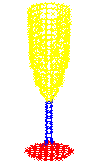
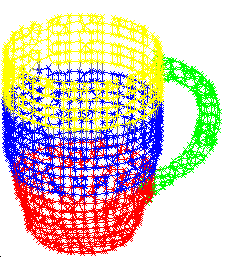
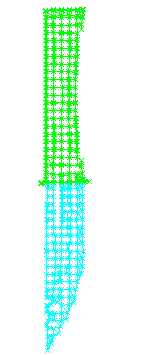
In addition, we consider the object database db, introduced in Neumann13mlg. db is a collection of $41$ simulated 3d point clouds of household objects. Each object is represented by a labeled graph where nodes represent points, labels are semantic parts (top, middle, bottom, handle, and usable-area), and the graph structure is given by a $k$-nearest neighbor ($k$-nn) graph w.r.t. Euclidean distance of the points in 3d space, cf. Figure 4(c). We further endowed each node with a continuous curvature attribute approximated by its derivative, that is, by the tangent plane orientations of its incident nodes. The attribute of node $u$ is given by $x_{u}=\sum_{v\in\mathcal{N}(u)}1-|\mathbf{n}_{u}\cdot\mathbf{n}_{v}|$, where $\mathbf{n}_{u}$ is the normal of point $u$ and $\mathcal{N}(u)$ are the neighbors of node $u$. The classification task here is to predict the category of each object. Examples of the $11$ categories are glass, cup, pot, pan, bottle, knife, hammer, and screwdriver.

Grid Graphs

We consider a classical benchmark dataset for texture classification (brodatz) and a dataset for plant disease classification (plants). All graphs in these datasets are grid graphs derived from pixel images. That is, the nodes are image pixels connected according to circular symmetric neighbor sets $N_{r,p}$ as exemplified in Eq. (29). Node labels are computed from the rgb color values by quantization.

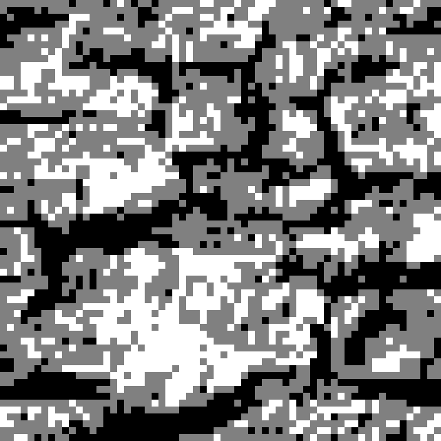
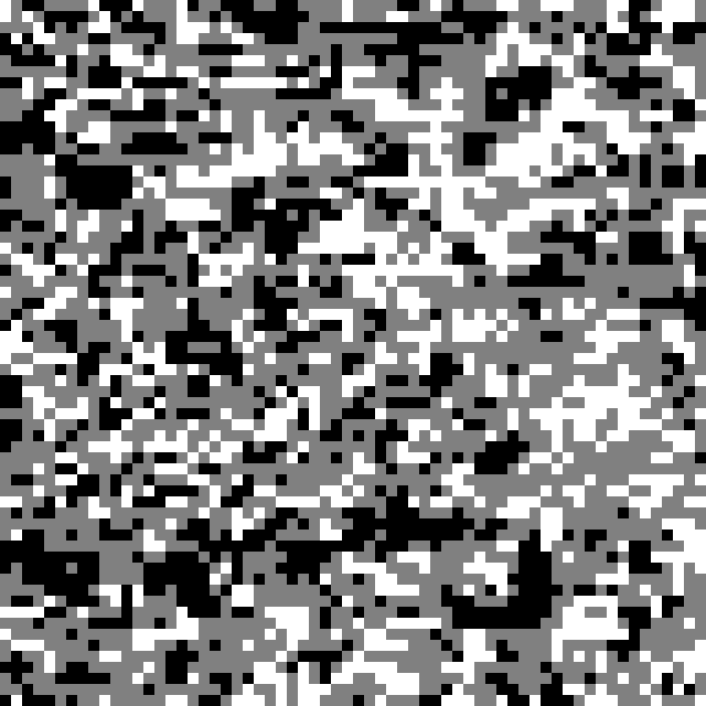
brodatz, introduced in ValkealahtiO98, covers 32 textures from the Brodatz album with 64 images per class comprising the following subsets of images: 16 “original” images (o), 16 rotated versions (r), 16 scaled versions (s), and 16 rotated and scaled versions (rs) of the “original” images. Figure 5(a) and (b) show example images with their corresponding quantized versions (e) and (f). For parameter learning, we used a random subset of 20% of the original images and their rotated versions, and for evaluation we use test suites similar to the ones provided with the dataset. All train/test splits are created such that whenever an original image (o) occurs in one split, their modified versions (r,s,rs) are also included in the same split.

The images in plants, introduced in NeumannHKKB14, are regions showing disease symptoms extracted from a database of $495$ rgb images of beet leaves. The dataset has six classes: five disease symptoms cercospora, ramularia, pseudomonas, rust, and phoma, and one class for extracted regions not showing a disease symptom. Figure 5(c) and (d) illustrates two regions and their quantized versions (g) and (h). We follow the experimental protocol in NeumannHKKB14 and use $10\%$ of the full data covering a balanced number of classes ($296$ regions) for parameter learning and the full dataset for evaluation. Note that this dataset is highly imbalanced, with two infrequent classes accounting for only $2\%$ of the examples and two frequent classes covering $35\%$ of the examples.

(a) bark

(b) grass

(c) phoma

(d) cercospora

(e) bark-3

(f) grass-3

(g) phoma-5

(h) cercospora-5

Figure 5: Example images from brodatz (a,b) and plants (c,d) and the corresponding quantized versions with 3 colors (e,f) and 5 colors (g,h).

7.2 Experimental Protocol

We implemented propagation kernels in Matlab and classification performance on all datasets except for db is evaluated by running c-svm classifications using libSVM. For the sensitivity analysis, the cost parameter $c$ was set to its default value of 1 for all datasets, whereas for the experimental comparison with existing graph kernels, we learned it via 5-fold cross-validation on the training set for all methods. The number of kernel iterations $t_{\textsc{max}}$ was learned on the training splits. Reported accuracies are an average of $10$ reruns of a stratified $10$-fold cross-validation.

For db, we follow the protocol introduced in Neumann13mlg. We perform a leave-one-out (loo) cross validation on the 41 objects in db, where the kernel parameter $t_{\textsc{max}}$ is learned on each training set again via loo. We further enhanced the nodes by a standardized continuous curvature attribute, which was previously only encoded in the edge weights. For all pks, the lsh bin-width parameters were set to $w_{l}=10^{-5}$ for labels and to $w_{a}=1$ for the normalized attributes, and as lsh metrics we chose $\textsc{m}_{l}=\textsc{tv}$ and $\textsc{m}_{a}=\textsc{l1}$ in all experiments. Before we evaluate classification performance and runtimes of the proposed propagation kernels, we analyze their sensitivity towards the choice of kernel parameters and with respect to missing and noisy observations.

7.3 Parameter Analysis

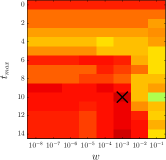
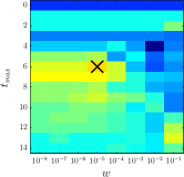
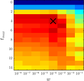
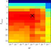
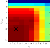
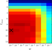
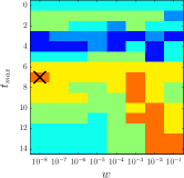
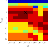
To analyze parameter sensitivity with respect to the kernel parameters $w$ (lsh bin width) and $t_{\textsc{max}}$ (number of kernel iterations), we computed average accuracies over 10 randomly generated test sets for all combinations of $w$ and $t_{\textsc{max}}$, where $w\in\{10^{-8},10^{-7},\dots,10^{-1}\}$ and $t_{\textsc{max}}\in\{0,1,\dots,14\}$ on mutag, enzymes, nci1, and db. The propagation kernel computation is as described in Algorithm 3, that is, we used the label information on the nodes and the label diffusion process as propagation scheme. To assess classification performance, we first learn the svm cost parameter on the full dataset for each parameter combination and then performed a 10-fold cross validation (cv). Further, we repeated each of these experiments with the normalized kernel, where normalization means dividing each kernel value by the square root of the product of the respective diagonal entries. Note that for normalized kernels we test for larger svm cost values. Figure 6 shows heatmaps of the results.

(a) mutag

(b) mutag,normalized

(c) enzymes

(d) enzymes, normalized

(e) nci1

(f) nci1,normalized

(g) db

(h) db,normalized

Figure 6: Parameter Sensitivity of pk. The plots show heatmaps of average accuracies (10-fold cv) of pk (labels only) w.r.t. the bin widths parameter $w$ and the number of kernel iterations $t_{\textsc{max}}$ for four datasets mutag, enzymes, nci1, and db. In panels (a, c, e, g) we used the kernel matrix directly, in panels (b, d, f, h) we normalized the kernel matrix. The svm cost parameter is learned for each combination of $w$ and $t_{\textsc{max}}$ on the full dataset. $\boldsymbol{\times}$ marks the highest accuracy.

In general, we see that the pk performance is relatively smooth, especially if $w<10^{-3}$ and $t_{\textsc{max}}>4$. Specifically, the number of iterations leading to the best results are in the range from $\{4,\dots,10\}$ meaning that we do not have to use a larger number of iterations in the pk computations, helping to keep a low computation time. This is especially important for parameter learning. Comparing the heatmaps of the normalized pk to the unnormalized pk leads to the conclusion that normalizing the kernel matrix can actually hurt performance. For mutag, Figure 6(a) and 6(b), the performance drops from $88.2\%$ to $82.9\%$, indicating that for this dataset the size of the graphs, or more specifically the amount of labels from the different kind of node classes, are a strong class indicator for the graph label. Nevertheless, incorporating the graph structure, i.e., comparing $t_{\textsc{max}}=0$ to $t_{\textsc{max}}=10$, can still improve classification performance by $1.5\%$. For other prediction scenarios such as the object category prediction on the db dataset, Figure 6(g) and 6(h), we actually want to normalize the kernel matrix to make the prediction independent of the object scale. That is, a cup scanned from a larger distance being represented by a smaller graph is still a cup and should be similar to a larger cup scanned from a closer view. So, for our experiments on object category prediction we will use normalized graph kernels whereas for the chemical compounds we will use unnormalized kernels unless stated otherwise.

In summary, we can answer (Q1) by concluding that pks are not overly sensitive to the choice of parameters and we propose to learn $t_{\textsc{max}}\in\{0,1,\dots,10\}$ and fix $w\leq 10^{-3}$. Further, we recommend to decide on using the normalized version of pks only when graph size invariance is deemed important for the classification task.

7.4 Comparison to Existing Graph Kernels

We compare classification accuracy and runtime of propagation kernels (pk) with the following state-of-the-art graph kernels: the Weisfeiler–Lehman subtree kernel (wl) ShervashidzeB11, the shortest path kernel (sp) borgwardtK05, the graph hopper kernel (gh) FeragenKPBB13, and the common subgraph matching kernel (csm) KriegeM12. Table 2 lists all graph kernels and the types of information they are intended for. For all wl computations, we used the fast implementation introduced in KerstingMGG14. In sp, gh, and csm, we used a Dirac kernel to compare node labels and a Gaussian kernel $k_{a}(u,v)=\exp(-\gamma\|x_{u}-x_{v}\|^{2})$ with $\gamma=\nicefrac{{1}}{{D}}$ for attribute information, if feasible. csm for the bigger datasets (enzymes, proteins, synthetic) was computed using a Gaussian truncated for inputs with $\|x_{u}-x_{v}\|>1$. We made this decision to encourage sparsity in the generated (node) kernel matrices, reducing the size of the induced product graphs and speeding up computation. Note that this is technically not a valid kernel between nodes; nonetheless, the resulting graph kernels were always positive definite. For pk and wl the number of kernel iterations ($t_{\textsc{max}}$ or $h_{\textsc{max}}$) and for csm the maximum size of subgraphs ($k$) was learned on the training splits via 10-fold cross validation. For all runtime experiments all kernels were computed for the largest value of $t_{\textsc{max}}$, $h_{\textsc{max}}$, or $k$, respectively. We used a linear base kernel for all kernels involving count features, and attributes, if present, were standardized. Further, we considered several baselines that do not take the graph structure into account. labels, corresponding to a pk with $t_{\textsc{max}}=0$, only compares the label proportions in the graphs, a takes the mean of a Gaussian node kernel among all pairs of nodes in the respective graphs, and a lsh again corresponds to a pk with $t_{\textsc{max}}=0$ using the attribute information only.

Table 2: Graph kernels and their intended use.

	information type
kernel	node	partial	edge	edge	node	grid graphs
	labels	labels	weights	labels	attributes	(fast scaling)
pk	yes	yes	yes	–	yes	yes
wl	yes	–	–	–	–	–
sp	yes	–	yes	yes	yes	–
gh	yes	–	yes	–	yes	–
csm	yes	–	yes	yes	yes	–

7.4.1 Graph Classification on Benchmark Data

In this section, we consider graph classification for fully labeled, partially labeled, and attributed graphs.

Fully Labeled Graphs

The experimental results for labeled graphs are shown in Table 3. On mutag, the baseline using label information only (labels) already gives the best performance indicating that for this dataset the actual graph structure is not adding any predictive information. On nci1 and nci109, wl performs best; however, propagation kernels come in second while being computed over one minute faster. Although sp can be computed quickly, it performs significantly worse than pk and wl. The same holds for gh, where for this kernel the computation is significantly slower. In general, the results on labeled graphs show that propagation kernels can be computed faster than state-of-the-art graph kernels but achieve comparable classification performance, thus question (Q4) can be answered affirmatively.

Table 3: Labeled Graphs. Average accuracies $\pm$ standard error of 10-fold cross validation (10 runs). Average runtimes in sec ($x^{\prime\prime}$), min ($x^{\prime}$), or hours ($xh$) are given in parentheses. The kernel parameters $t_{\textsc{max}}$ for pk and $h_{\textsc{max}}$ for wl were learned on the training splits ($t_{\textsc{max}},h_{\textsc{max}}\in\{0,1,\dots,10\}$). labels corresponds to pk with $t_{\textsc{max}}=0$. OUT OF TIME indicates that the kernel computation did not finish within $24$h. Bold indicates that the method performs significantly better than the second best method under a paired $t$-test ($p<0.05$).

	dataset
method	mutag	nci1	nci109	dd
pk	$84.5$ $\pm 0.6$ $(0.2^{\prime\prime})$	$84.5$ $\pm 0.1$ $(4.5^{\prime}$)	$83.5$ $\pm 0.1$ $(4.4^{\prime}$)	$78.8$ $\pm 0.2$ $(3.6^{\prime}$)
wl	$84.0$ $\pm 0.4$ $(0.2^{\prime\prime})$	$\mathbf{85.9}$ $\pm 0.1$ $(5.6^{\prime}$)	$\mathbf{85.9}$ $\pm 0.1$ $(7.4^{\prime}$)	$79.0$ $\pm 0.2$ $(6.7^{\prime}$)
sp	$85.8$ $\pm 0.2$ $(0.2^{\prime\prime})$	$74.4$ $\pm 0.1$ $(21.3^{\prime\prime})$	$73.7$ $\pm 0.0$ $(19.3^{\prime\prime})$	OUT OF TIME
gh	$85.4$ $\pm 0.5$ $(1.0^{\prime}$)	$73.2$ $\pm 0.1$ $(13.0$h)	$72.6$ $\pm 0.1$ $(22.1$h)	$68.9$ $\pm 0.2$ ($69.1$h)
labels	$85.8$ $\pm 0.2$ $(0.2^{\prime\prime})$	$64.6$ $\pm 0.0$ $(4.5^{\prime}$)	$63.6$ $\pm 0.0$ $(4.4^{\prime}$)	$78.4$ $\pm 0.1$ $(3.6^{\prime}$)

Partially Labeled Graphs

To assess the predictive performance of propagation kernels on partially labeled graphs, we ran the following experiments $10$ times. We randomly removed 20–80% of the node labels in all graphs in msrc9 and msrc21 and computed cross-validation accuracies and standard errors. Because the wl-subtree kernel was not designed for partially labeled graphs, we compare pk to two variants: one where we treat unlabeled nodes as an additional label “$u$” (wl) and another where we use hard labels derived from running label propagation (lp) until convergence (lp $+$ wl). The results are shown in Table 4. For larger fractions of missing labels, pk obviously outperforms the baseline methods, and, surprisingly, running label propagation until convergence and then computing wl gives slightly worse results than wl. However, label propagation might be beneficial for larger amounts of missing labels. The runtimes of the different methods on msrc21 are shown in Figure 8 in the Appendix. wl computed via the string-based implementation suggested in ShervashidzeB11 is over $36$ times slower than pk. These results again confirm that propagation kernels have attractive scalability properties for large datasets. The lp $+$ wl approach wastes computation time while running lp to convergence before it can even begin calculating the kernel. The intermediate label distributions obtained during the convergence process are already extremely powerful for classification. These results clearly show that propagation kernels can successfully deal with partially labeled graphs and suggest an affirmative answer to questions (Q3) and (Q4).

Table 4: Partially Labeled Graphs. Average accuracies (and standard errors) on $10$ different sets of partially labeled images for pk and wl with unlabeled nodes treated as additional label (wl) and with hard labels derived from converged label propagation (lp $+$ wl). Bold indicates that the method performs significantly better than the second best method under a paired $t$-test ($p<0.05$).

		labels missing
dataset	method	$20\%$	$40\%$	$60\%$	$80\%$
	pk	$90.0$ $\pm 0.4$	$88.7$ $\pm 0.3$	$86.6$ $\pm 0.4$	$80.4$ $\pm 0.6$
msrc9	lp $+$ wl	$90.0$ $\pm 0.2$	$87.9$ $\pm 0.6$	$83.2$ $\pm 0.6$	$77.9$ $\pm 1.0$
	wl	$89.2$ $\pm 0.5$	$88.1$ $\pm 0.5$	$85.7$ $\pm 0.6$	$78.5$ $\pm 0.9$
	pk	$\mathbf{86.9}$ $\pm 0.3$	$\mathbf{84.7}$ $\pm 0.3$	$\mathbf{79.5}$ $\pm 0.3$	$\mathbf{69.3}$ $\pm 0.3$
msrc21	lp $+$ wl	$85.8$ $\pm 0.2$	$81.5$ $\pm 0.3$	$74.5$ $\pm 0.3$	$64.0$ $\pm 0.4$
	wl	$85.4$ $\pm 0.4$	$81.9$ $\pm 0.4$	$76.0$ $\pm 0.3$	$63.7$ $\pm 0.4$

(a) synthetic

(b) enzymes

(c) bzr

(d) pro-full

Figure 7: Attributed Graphs – Log Runtime vs. Accuracy. The plots show log(runtimes) in seconds plotted against average accuracy ($\pm$ standard deviation). Methods are encoded by color and the used information (labels, attributes or both) is encoded by shape. Note that p2k also uses both, labels and attributes, however in contrast to pk both are propagated. For pro-full the csm kernel computation exceeded 32GB of memory. On synthetic csm using the attribute information only could not be computed within $72$h.

Attributed Graphs

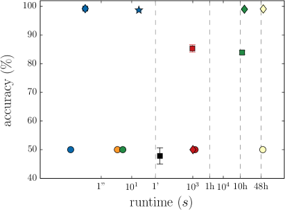
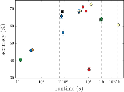
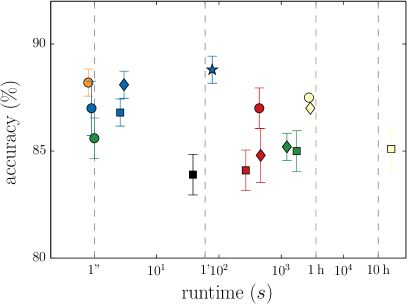
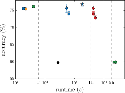
The experimental results for various datasets with attributed graphs are illustrated in Figure 7. The plots show runtime versus average accuracy, where the error bars reflect standard deviation of the accuracies. As we are interested in good predictive performance while achieving fast kernel computation, methods in the upper-left corners provide the best performance with respect to both quality and speed. For pk, sp, gh, and csm we compare three variants: one where we use the labels only, one where we use the attribute information only, and one where both labels and attributes are used. wl is computed with label information only. For synthetic, cf. Figure 7(a), we used the node degree as label information. Further, we compare the performance of p2k, which propagates labels and attributes as described in Section 6.3. Detailed results on synthetic and all bioinformatics datasets are provided in Table 8 (average accuracies) and Table 7 (runtimes) in the Appendix. From Figure 7 we clearly see that propagation kernels tend to appear in the upper-left corner, that is, they are achieving good predictive performance while being fast, leading to a positive answer of question (Q4). Note that the runtimes are shown on a log scale. We can also see that p2k, propagating both labels and attributes, (blue star) usually outperforms the the simple pk implementation not considering attribute arrangements (blue diamond). However, this comes at the cost of being slower. So, we can use the flexibility of propagation kernels to trade predictive quality against speed or vice versa according to the requirements of the application at hand. This supports a positive answer to question (Q3).

7.4.2 Graph Classification on Novel Applications

The flexibility of propagation kernels arising from easily interchangeable propagation schemes and their efficient computation via lsh allows us to apply graph kernels to novel domains. First, we are able to compare larger graphs with reasonable time expended, opening up the use of graph kernels for object category prediction of 3d point clouds in the context of robotic grasping Neumann13mlg. Depending on their size and the perception distance, point clouds of household objects can easily consist of several thousands of nodes. Traditional graph kernels suffer from enormous computation times or memory problems even on datasets like db, which can still be regarded medium sized. These issues aggravate even more when considering image data. So far, graph kernels have been used for image classification on the scene level where the nodes comprise segments of similar pixels and one image is then represented by less than 100 so-called superpixels. Utilizing off-the-shelf techniques for efficient diffusion on grid graphs allows the use of propagation kernels to analyze images on the pixel level and thus opens up a whole area of interesting problems in the intersection of graph-based machine learning and computer vision. As a first step, we apply graph kernels, more precisely propagation kernels, to texture classification, where we consider datasets with thousands of graphs containing a total of several millions of nodes.

3d Object Category Prediction

In this set of experiments, we follow the protocol introduced in Neumann13mlg, where the graph kernel values are used to derive a prior distribution on the object category for a given query object. The experimental results for the 3d-object classification are summarized in Table 5. We observe that propagation kernels easily deal with the point-cloud graphs. From the set of baseline graph kernels considered, only wl was feasible to compute, however with poor performance. Propagation kernels clearly benefit form their flexibility as we can improve the classification accuracy from $75.4\%$ to $80.7\%$ when considering the object curvature attribute. These results are extremely promising given that we tackle a classification problem with 11 classes having only 40 training examples for each query object.

Table 5: Point Cloud Graphs. Average accuracies of loo cross validation on db. The reported standard errors refer to 10 kernel recomputations. Runtimes are given in sec ($x^{\prime\prime}$). The kernel parameters, $t_{\textsc{max}}$ for all pks and $h_{\textsc{max}}$ for wl, were learned on the training splits ($t_{\textsc{max}},h_{\textsc{max}}\in\{0,\dots 15\}$). a lsh corresponds to pk with $t_{\textsc{max}}=0$. sp, gh, and csm were either OUT OF MEMORY or the computation did not finish within $24$h for all settings.

	labels		labels
			attr		attr
	pk	wl	pk	p2k	a	a lsh
acc$\pm$stderr	$75.6\pm 0.6$	$70.7\pm 0.0$	$76.8\pm 1.3$	$\mathbf{82.9}\pm 0.0$	$36.4\pm 0.0$	$63.4\pm 0.0$
runtime	$0.2^{\prime\prime}$	$0.4^{\prime\prime}$	$0.3^{\prime\prime}$	$34.8^{\prime\prime}$	$40.0^{\prime\prime}$	$0.0^{\prime\prime}$

Grid Graphs

For brodatz and plants we follow the experimental protocol in NeumannHKKB14. The pk parameter $t_{\textsc{max}}$ was learned on a training subset of the full dataset ($t_{\textsc{max}}\in\{0,3,5,8,10,15,20\}$). For plants this training dataset consists of 10% of the full data; for brodatz we used 20% of the brodatz-o-r data as the number of classes in this dataset is much larger (32 textures). We also learned the quantization values ($col\in\{3,5,8,10,15\}$) and neighborhoods ($B\in\{N_{1,4}$, $N_{1,8}$, $N_{2,16}\}$, cf. Eq. (29)). For brodatz the best performance on the training data was achieved with $3$ colors and a 8-neighborhood, whereas for plants $5$ colors and the 4-neighborhood was learned. We compare pk to the simple baseline labels using label counts only and to a powerful second-order statistical feature based on the gray-level co-occurrence matrix haralick73 comparing intensities (glcm-gray) or quantized labels (glcm-quant) of neighboring pixels.

The experimental results for grid graphs are shown in Table 6. While not outperforming sophisticated and complex state-of-the-art computer vision approaches to texture classification, we find that it is feasible to compute pks on huge image datasets achieving respectable performance out of the box. This is – compared to the immense tuning of features and methods commonly done in computer vision – a great success. On plants, pk achieves an average accuracy of $82.5\%$, where the best reported result so far is $83.7\%$, which was only achieved after tailoring a complex feature ensemble NeumannHKKB14. In conclusion, propagation kernels are an extremely promising approach in the intersection of machine learning, graph mining, and computer vision.

Table 6: Grid Graphs. Average accuracies $\pm$ standard errors of 10-fold cv (10 runs). The pk parameter $t_{\textsc{max}}$ as well as color quantization and pixel neighborhood was learned on a training subset of the full dataset. Average runtimes in sec ($x^{\prime\prime}$) or min ($x^{\prime}$) given in parentheses refer to the learned parameter settings. For glcm-quant and labels the same color quantization as for pk was applied. labels corresponds to pk with $t_{\textsc{max}}=0$. brodatz-o-r is using the original images and their 90 degree rotated versions and brodatz-o-r-s-rs additionally includes their scaled, and scaled and rotated versions.

	dataset
method	brodatz-o-r	brodatz-o-r-s-rs	plants
pk	$\mathbf{89.6}$ $\pm 0.0$ ($3.5^{\prime}$)	$\mathbf{85.7}$ $\pm 0.0$ ($7.1^{\prime}$)	$\mathbf{82.5}$ $\pm 0.1$ ($3.0^{\prime}$)
labels	$5.0$ $\pm 0.0$ ($1.1^{\prime}$)	$4.9$ $\pm 0.0$ ($2.2^{\prime}$)	$59.5$ $\pm 0.0$ ($11.5^{\prime\prime}$)
glcm-gray	$87.2$ $\pm 0.0$ ($29.5^{\prime\prime}$)	$79.4$ $\pm 0.0$ ($44.8^{\prime\prime}$)	$76.6$ $\pm 0.0$ ($1.4^{\prime}$)
glcm-quant	$78.6$ $\pm 0.0$ ($24.9^{\prime\prime}$)	$68.6$ $\pm 0.0$ ($44.8^{\prime\prime}$)	$37.5$ $\pm 0.0$ ($1.1^{\prime}$)

Summarizing all experimental results, the capabilities claimed in Table 2 are supported. Propagation kernels have proven extremely flexible and efficient and thus question (Q3) can ultimately be answered affirmatively.

8 Conclusion

Random walk-based models provide a principled way of spreading information and even handling missing and uncertain information within graphs. Known labels are, for example, propagated through the graph in order to label all unlabeled nodes. In this paper, we showed how to use random walks to discover structural similarities shared between graphs for the construction of a graph kernel, namely the propagation kernel. Intuitively, propagation kernels count common sub-distributions induced in each iteration of running inference in two graphs leading to the insight that graph kernels are much closer to graph-based learning than assumed before.

As our experimental results demonstrate, propagation kernels are competitive in terms of accuracy with state-of-the-art kernels on several classification benchmark datasets of labeled and attributed graphs. In terms of runtime, propagation kernels outperform all recently developed efficient and scalable graph kernels. Moreover, being tied to the propagation scheme, propagation kernels can be easily adapted to novel applications not having been tractable for graph kernels before.

Propagation kernels provide several interesting avenues for future work. While we have used classification to guide the development of propagation kernels, the results are directly applicable to regression, clustering, and ranking, among other tasks. Employing message-based probabilistic inference schemes such as (loopy) belief propagation directly paves the way to dealing with graphical models. Exploiting that graph kernels and graph-based learning (learning on the node level) are closely related, a natural extension to this work is the derivation of a unifying propagation-based framework for structure representation independent of the learning task being on the graph or node level.

Appendix A Runtimes for Partially Labeled Graphs

Figure 8: Runtime for Partially Labeled msrc21. Avg. time in secs over $10$ instances of the msrc21 dataset with $50\%$ labeled nodes for kernel iterations from $0$ to $10$. We compare pk to wl with unlabeled nodes treated as additional label and with hard labels derived from converged label propagation (lp$+$wl).

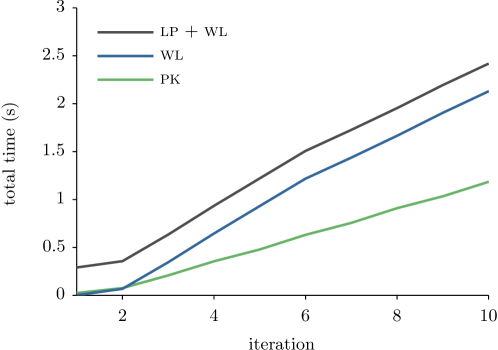
Appendix B Detailed Results on Attributed Graphs

Table 7: Attributed Graphs – Runtimes. Kernel computation times (cputime) are given in sec ($x^{\prime\prime}$), min ($x^{\prime}$), or hours ($x$h). For all pks, $t_{\textsc{max}}=10$; for wl, $h_{\textsc{max}}=10$; and for csm, $k=7$. All computations are performed on machines with 3.4 GHz Intel core i7 processors. Note that csm is implemented in Java, so comparing computation times is only possible to a limited extent. OUT OF TIME means that the computation did not finish within $72$h.

			dataset
method			synthetic	enzymes	proteins	pro_full	bzr	cox2	dhfr
labels		pk	$\mathbf{0.1^{\prime\prime}}$	$\mathbf{3.6^{\prime\prime}}$	$\mathbf{17.8^{\prime\prime}}$	$\mathbf{18.7^{\prime\prime}}$	$0.9^{\prime\prime}$	$1.1^{\prime\prime}$	$3.4^{\prime\prime}$
		wl	$3.4^{\prime\prime}$	$4.1^{\prime\prime}$	$25.9^{\prime\prime}$	$22.2^{\prime\prime}$	$\mathbf{0.8^{\prime\prime}}$	$1.0^{\prime\prime}$	$4.2^{\prime\prime}$
		sp	$5.1^{\prime\prime}$	$1.3^{\prime\prime}$	$38.7^{\prime\prime}$	$40.3^{\prime\prime}$	$1.0^{\prime\prime}$	$1.2^{\prime\prime}$	$\mathbf{2.3^{\prime\prime}}$
		gh	$19.8^{\prime}$	$17.8^{\prime}$	$2.2$h	$1.4$h	$7.4^{\prime}$	$10.8^{\prime}$	$29.5^{\prime}$
		csm	$54.8$h	$5.2$h	–	–	$46.4^{\prime}$	$1.6$h	$3.7$h
	attr	pk	$\mathbf{0.3^{\prime\prime}}$	$\mathbf{1.4^{\prime}}$	$\mathbf{23.6^{\prime\prime}}$	$\mathbf{10.7^{\prime}}$	$\mathbf{2.6^{\prime\prime}}$	$\mathbf{2.8^{\prime\prime}}$	$\mathbf{14.8^{\prime\prime}}$
		sp	$11.5$h	$55.4^{\prime}$	$5.9$h	$6.0$h	$29.5^{\prime}$	$25.9^{\prime}$	$1.3$h
		gh	$16.2^{\prime}$	$13.2^{\prime}$	$1.9$h	$72.4^{\prime}$	$4.5^{\prime}$	$6.6^{\prime}$	$15.8^{\prime}$
		csm	OUT OF TIME	$7.6^{\prime}$	–	–	$16.2$h	$31.5$h	$97.5$h
labels	attr	pk	$\mathbf{0.3^{\prime\prime}}$	$\mathbf{1.2^{\prime}}$	$\mathbf{20.0^{\prime\prime}}$	$\mathbf{9.0^{\prime}}$	$\mathbf{3.0^{\prime\prime}}$	$\mathbf{3.5^{\prime\prime}}$	$\mathbf{15.1^{\prime\prime}}$
		p2k	$17.2^{\prime\prime}$	$6.7^{\prime}$	$31.4^{\prime}$	$30.6^{\prime}$	$1.3^{\prime}$	$1.8^{\prime}$	$5.9^{\prime}$
		sp	$13.7$h	$1.0$h	$6.8$h	$7.0$h	$20.5^{\prime}$	$32.9^{\prime}$	$1.6$h
		gh	$16.9^{\prime}$	$9.8^{\prime}$	$1.2$h	$1.2$h	$7.8^{\prime}$	$11.7^{\prime}$	$31.2^{\prime}$
		csm	$56.8$h	$21.8^{\prime}$	–	–	$48.8^{\prime}$	$1.6$h	$3.7$h
	attr	a	$1.4^{\prime}$	$1.3^{\prime}$	$6.4^{\prime}$	$4.6^{\prime}$	$38.3^{\prime\prime}$	$1.1^{\prime}$	$3.2^{\prime}$

Table 8: Attributed Graphs – Accuracies. Average accuracies $\pm$ standard error of 10-fold cross validation (10 runs). All pks were also recomputed for each run as there is randomization in the lsh computation. The kernel parameters $t_{\textsc{max}}$ for all pks and $h_{\textsc{max}}$ for wl were learned on the training splits ($t_{\textsc{max}},h_{\textsc{max}}\in\{0,1,\dots 10\}$). For all pks we applied standardization to the attributes and one hash per attribute dimension is computed. Whenever the normalized version of a kernel performed better than the unnormalized version we report these results and mark the method with $\ast$. csm is implemented in Java and computations were performed on a machine with 32gb of memory. OUT OF MEMORY indicates a Java outOfMemeoryError. Bold indicates that the method performs significantly better than the second best method under a paired $t$-test ($p<0.05$). The svm cost parameter is learned on the training splits. We choose $c\in\{10^{-7},10^{-5},\cdots 10^{5},10^{7}\}$ for normalized kernels and $c\in\{10^{-7},10^{-5},10^{-3},10^{-1}\}$ for unnormalized kernels.

			dataset
method			synthetic	enzymes	proteins	pro-full	bzr	cox2	dhfr
labels		pk	$50.0$ $\pm 0.0^{\ast}$	$46.0$ $\pm 0.3$	$75.6$ $\pm 0.1^{\ast}$	$75.6$ $\pm 0.1^{\ast}$	$87.0$ $\pm 0.4$	$81.0$ $\pm 0.2$	$83.5$ $\pm 0.2^{\ast}$
		wl	$50.0$ $\pm 0.0^{\ast}$	$46.3$ $\pm 0.2^{\ast}$	$75.5$ $\pm 0.1^{\ast}$	$75.5$ $\pm 0.1^{\ast}$	$88.2$ $\pm 0.2$	$\mathbf{83.2}$ $\pm 0.2^{\ast}$	$84.1$ $\pm 0.2$
		sp	$50.0$ $\pm 0.0^{\ast}$	$40.4$ $\pm 0.3^{\ast}$	$76.2$ $\pm 0.1^{\ast}$	$76.2$ $\pm 0.1^{\ast}$	$85.6$ $\pm 0.3$	$81.0$ $\pm 0.4^{\ast}$	$82.0$ $\pm 0.3^{\ast}$
		gh	$50.0$ $\pm 0.0^{\ast}$	$34.8$ $\pm 0.4^{\ast}$	$72.9$ $\pm 0.2^{\ast}$	$72.9$ $\pm 0.2^{\ast}$	$87.0$ $\pm 0.3$	$81.4$ $\pm 0.3^{\ast}$	$79.5$ $\pm 0.4$
		csm	$50.0$ $\pm 0.0^{\ast}$	$60.83$ $\pm 0.2$	OUT OF MEMORY	OUT OF MEMORY	$87.5$ $\pm 0.2^{\ast}$	$80.7$ $\pm 0.3$	$82.6$ $\pm 0.2^{\ast}$
	attr	pk	$99.2$ $\pm 0.1^{\ast}$	$56.4$ $\pm 0.6$	$72.7$ $\pm 0.2$	$74.1$ $\pm 0.2^{\ast}$	$86.8$ $\pm 0.2^{\ast}$	$78.2$ $\pm 0.4$	$84.3$ $\pm 0.1$
		sp	$83.9$ $\pm 0.2^{\ast}$	$63.9$ $\pm 0.3^{\ast}$	$74.3$ $\pm 0.1^{\ast}$	$59.9$ $\pm 0.0^{\ast}$	$85.0$ $\pm 0.3^{\ast}$	$78.2$ $\pm 0.0$	$78.9$ $\pm 0.3^{\ast}$
		gh	$85.3$ $\pm 0.4$	$68.8$ $\pm 0.2^{\ast}$	$72.6$ $\pm 0.1^{\ast}$	$61.2$ $\pm 0.0^{\ast}$	$84.1$ $\pm 0.3^{\ast}$	$79.5$ $\pm 0.2^{\ast}$	$79.0$ $\pm 0.2$
		csm	–	$68.9$ $\pm 0.2^{\ast}$	OUT OF MEMORY	OUT OF MEMORY	$85.1$ $\pm 0.3^{\ast}$	$77.6$ $\pm 0.3$	$79.5$ $\pm 0.2$
labels	attr	pk	$99.2$ $\pm 0.1^{\ast}$	$65.9$ $\pm 0.4^{\ast}$	$76.3$ $\pm 0.2^{\ast}$	$75.7$ $\pm 0.4^{\ast}$	$88.1$ $\pm 0.2^{\ast}$	$79.4$ $\pm 0.6$	$84.1$ $\pm 0.3^{\ast}$
		p2k	$98.7$ $\pm 0.1$	$68.1$ $\pm 0.5$	$75.9$ $\pm 0.2^{\ast}$	$\mathbf{76.9}$ $\pm 0.2^{\ast}$	$88.8$ $\pm 0.2$	$80.9$ $\pm 0.4$	$83.5$ $\pm 0.3^{\ast}$
		sp	$99.0$ $\pm 0.1$	$64.3$ $\pm 0.3^{\ast}$	$73.2$ $\pm 0.2^{\ast}$	$59.9$ $\pm 0.0^{\ast}$	$85.2$ $\pm 0.2^{\ast}$	$78.5$ $\pm 0.1$	$79.7$ $\pm 0.2^{\ast}$
		gh	$50.0$ $\pm 0.0^{\ast}$	$71.2$ $\pm 0.2^{\ast}$	$73.0$ $\pm 0.1^{\ast}$	$60.9$ $\pm 0.0^{\ast}$	$84.8$ $\pm 0.4$	$79.5$ $\pm 0.2^{\ast}$	$80.0$ $\pm 0.2$
		csm	$99.0$ $\pm 0.1$	$\mathbf{72.8}$ $\pm 0.4^{\ast}$	OUT OF MEMORY	OUT OF MEMORY	$87.0$ $\pm 0.2^{\ast}$	$79.2$ $\pm 0.4^{\ast}$	$80.1$ $\pm 0.3^{\ast}$
	attr	a	$47.8$ $\pm 0.9^{\ast}$	$68.5$ $\pm 0.2^{\ast}$	$72.8$ $\pm 0.2^{\ast}$	$59.8$ $\pm 0.0^{\ast}$	$83.9$ $\pm 0.3^{\ast}$	$78.2$ $\pm 0.0$	$74.8$ $\pm 0.2^{\ast}$