Variable Stars in Metal-Rich Globular Clusters. IV. Long Period Variables in NGC 6496

Abstract

We present $VI$-band photometry for stars in the metal-rich globular cluster NGC 6496. Our time-series data were cadenced to search for long period variables (LPVs) over a span of nearly two years, and our variability search yielded the discovery of thirteen new variable stars, of which six are LPVs, two are suspected LPVs, and five are short period eclipsing binaries. An additional star was found in the ASAS database, and we clarify its type and period. We argue that all of the eclipsing binaries are field stars, while 5-6 of the LPVs are members of NGC 6496. We compare the period-luminosity distribution of these LPVs with those of LPVs in the Large Magellanic Cloud and 47 Tucanae, and with theoretical pulsation models. We also present a $VI$ color magnitude diagram, display the evolutionary states of the variables, and match isochrones to determine a reddening of $E(B-V)=0.21\pm 0.02$ mag and apparent distance modulus of $15.60\pm 0.15$ mag.

1 Introduction

Models of stellar structure and evolution for low-mass stars have been developed and improved using observational data of globular clusters (e.g., Sweigart & Catelan 1998; Piotto et al. 2007). For instance, observing a globular cluster in two or more bands allows an observer to obtain the color-magnitude diagram (CMD). Comparing the CMD to isochrones yields the locations and shapes of the principle sequences, which can be used to refine the theoretical treatment of stellar interiors. Additionally, matching the observed CMD to isochrones provides information about the metallicity and age of the observed globular cluster. In a similar way, comparisons of observed stellar pulsation properties (periods, amplitudes, surface velocities, etc.) with the predictions of theoretical models of stellar pulsation can provide additional constraints on the properties of stellar interiors and evolution (e.g., Smith 1995; Olivier & Wood 2005; Lebzelter & Wood 2005).

To obtain such data, time series observations are needed to detect variable stars and follow their properties over multiple pulsation cycles. Previous variability studies of globular clusters focused on short period variable stars such as RR Lyrae stars, SX Phoenicis stars, etc., as the time series observations could be acquired during a classically-scheduled observing run. It is more challenging and time consuming to detect long period variables (LPVs) as they have periods ranging from 30-1000 days, but the new generation or robotic telescopes have enabled multi-year campaigns with short and regular observing cadences.

Typically, LPVs are divided into Mira, Semiregular, and Irregular classes, forming a continuum in descending order of period length, amplitude size, and regularity of cyclicity. These stars are in their last stage of stellar evolution, on the asymptotic giant branch (AGB), and are forming dust and ejecting gas while pulsating. Understanding the pulsation and properties of these stars can help us improve our understanding of theoretical stellar pulsation and evolution along with the process of chemical enrichment of the interstellar medium.

As part of a survey for RR Lyrae stars in metal rich globular clusters (Layden et al., 1999, 2003; Baker et al., 2007), we present multi-band, multi-epoch observations obtained for the metal-rich globular cluster NGC 6496 (C1755-442). This cluster is located at galactic coordinates ($l$, $b$) = (348.03°, –10.01°), at a distance $\sim$11.3 kpc from the Sun. The moderate latitude comes with a modest level of foreground reddening, $E(B-V)=0.15$ mag, and field-star contamination. The cluster has a relatively metal-rich composition of [Fe/H] = –0.46 (Harris, 1996), leading Zinn (1985) to list it as a member of the galactic thick disk population, though Richtler et al. (1994) provided counter evidence. The cluster has an open, uncroweded nature (structural parameters include core, half-mass, and tidal radii of 0.95, 1.02, and 4.8 arcmin, respectively) making NGC 6496 a good candidate for CCD photometry with a telescope of modest plate scale. However, the faint integrated light of the cluster after conversion to absolute magnitude, $M_{V}=-7.2$ mag (Harris, 1996), and its consequent low integrated stellar mass indicate that a small population of variable stars is to be expected. Previous searches for variable stars in the cluster found no candidates (Clement et al., 2001). In particular, the photographic survey by Fourcade & Laborde (1966) yielded no clear variable stars. A lack of RR Lyrae variables in NGC 6496 is no surprise given the cluster’s relatively high metallicity and red-clump horizontal branch morphology (Armandroff, 1988; Richtler et al., 1994; Sarajedini & Norris, 1994), but the high metallicity favors the formation of long period variables (for example, Frogel & Whitelock (1998) showed that luminous LPVs are found only in clusters with [Fe/H] $>-1.0$), and so a modern search seems warranted.

In this paper, we present new time-series images in Section 2, our photometric analysis of these data in Sec. 3, and the resulting color-magnitude diagrams in Sec. 4. We discuss the detection, properties and membership likelihood of the variable stars in Sec. 5, and compare them with similar variables in the Large Magellanic Cloud and the metal-rich globular cluster 47 Tucanae. We summarize our findings in Sec. 6.

2 Observations and Reductions

As part of the original survey for RR Lyrae stars in metal-rich globular clusters, we obtained time-series images of NGC 6496 using the direct CCD camera on the 0.9-m telescope at Cerro Tololo Inter-American Observatory (CTIO) during two runs in May and June of 1996 having 1 and 7 usable nights, respectively. The Tek#3 2048 CCD, operated with a gain of 2.4 electrons/adu and a readout noise of 3.7 electrons, provided a $13.5\arcmin$ field of view with $0.4\arcsec$ pixels. We used filters matched to the CCD to reproduce the Johnson $V$ and Kron-Cousins $I$ bandpasses. The raw images were processed using the Image Reduction and Analysis Facility (IRAF) to perform the standard procedures for overscan subtraction and bias correction, and by using twilight sky frames to flat-field the images.

In a typical pointing toward the cluster, we obtained a short exposure (25–120 s) $VI$ frame pair and a long exposure (250–350 s) $VI$ pair. Such pointings were obtained 1–2 times each night, with time intervals between pointings of at least five hours. In total, we obtained 48 images in twelve pointings (independent photometric epochs) toward NGC 6496. The seeing varied between 1.0$\arcsec$ and 4.5$\arcsec$ (1.9$\arcsec$ median) fwhm, with 19% of the images having seeing greater than 2.5$\arcsec$. Preliminary photometry using the CTIO images indicated the presence of at least five slow, red variables, and at least five stars with variations on shorter timescales. However, the sampling was insufficient to determine the nature of these variables.

Additional observations were obtained using the 0.41-m Panchromatic Robotic Optical Monitoring and Polarimetry Telescope number 4 (PROMPT4; Reichart et al. 2005). This telescope is equipped with a 1k$\times$1k Apogee CCD camera (Nysewander et al., 2009) with a 10$\arcmin$ field of view and a 0.59$\arcsec$ pixel size (Reichart et al., 2005). The CCD has a gain of 1.5 electrons/adu and readout noise of 13.5 electrons. On $\sim$63 nights that span almost two years (February 2009 through October 2010) and that are each separated by 1-2 weeks, we obtained images of NGC 6496 through standard $V$ and $I$ filters. On each night, we obtained four 80 s images in $V$, three 40 s images in $I$, and three 10 s images in $I$ (hereafter referred to as $I_{L}$ and $I_{S}$, for “long” and “short,” respectively). The images were taken in the order “$V$, $I_{L}$, $I_{S}$; $V$, $I_{L}$, $I_{S}$; $V$, $I_{L}$, $I_{S}$; $V$” so that small tracking errors would shift stars across several pixels, providing de facto dithering that would later allow us to reject bad pixels and cosmic rays. The long and short exposure $I$ images allowed us to maximize dynamic range in the resulting photometry, and ensure that bright LPVs were not saturated when observed at maximum light. The seeing varied between 1.2 and 3.5$\arcsec$ fwhm with a median of 1.9$\arcsec$, and with 13% of the 188 individual P4 images having seeing greater than 2.5$\arcsec$.

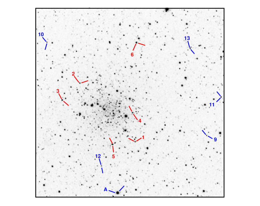
Figure 1: The combined $V$-band master image of NGC 6496 taken with PROMPT4. North is up and East is to the left. The axes of the $10\times 10$ arcmin field of view go from $X_{pix}=1$ to 1024 pix from left to right, and from $Y_{pix}=1$ to 1024 pix from bottom to top. The uncrowded nature of the cluster helped us obtain good photometry even near the cluster center. Variable stars are marked with their assigned numbers (e.g., ”1” indicates ”V1”), while “A” marks the variable star ASAS 175901-4411.5. In the electronic edition, red and blue symbols mark long and short period stars, respectively.

The raw cluster images and suitable calibration images from each observing night were retrieved from the PROMPT website and processed using IRAF packages to correct for bias patterns, dark current, and flatness-of-field variations. After inspecting the set of four processed $V$ images from each pointing and rejecting any poor-quality ones, the remaining images where shifted and combined to produce a single, high signal-to-noise (S/N) $V$ image that is devoid of bad pixels and cosmic rays. Similar steps were followed separately for the three $I_{L}$ images and for the three $I_{S}$ images, yielding three final images for each observing night. One such image, the combined $V$ frame taken on 2009-08-20, is shown in Figure 1. Note the open nature of the cluster, and the significant field star population. Together, the CTIO and PROMPT images provided up to 77 independent photometric epochs in each band for each variable star in our data set.

3 DAOPHOT Photometry

Instrumental photometry of the CTIO 0.9-m images was performed using the DAOPHOT II (Stetson, 1987) and ALLFRAME (Stetson, 1994) packages following the procedures described in (Baker et al., 2007). Hereafter, we refer to this as the “CTIO” photometry set.

These packages were used in a similar way to do photometry on the PROMPT4 images (hereafter referred to as the “P4” photometry set). The FIND and PHOT routines of DAOPHOT II were used to detect and provide initial aperture photometry of objects above a threshold on each image. We then used PICK to select $\sim$160 bright stars located away from the cluster center to determine the stellar point-spread function (PSF), and the PSF routine was used to combine all the PSF stars’ profiles into a single PSF model for each image. The ALLSTAR program then fit the PSF model to all of the stars in each processed image and gives an improved estimation of the stars’ locations and magnitudes. An automatic, iterative procedure was used to subtract the light of stars located near the PSF stars and build an improved PSF, which was run again through ALLSTAR to further improve the photometry for that image.

We then selected the best ten $V$ images and combined them using MONTAGE to create a deep image with high S/N that can be used as a reference image. The DAOPHOT and ALLSTAR procedures were then applied to the MONTAGE image to get a master reference list that contains the locations and average magnitudes of all sources found in the MONTAGE. Similarly, MONTAGE images and master star lists were created from the $I_{L}$ and $I_{S}$ image sets.

The DAOMASTER program was used to match the same stars in different images. Using the master list of stellar positions, the ALLFRAME program was used (separately for the $V$, $I_{L}$ and $I_{S}$ sets) to obtain final instrumental photometry for objects on each frame. The systematic use of a single master star list reduces the confusion in crowded environments that can lead to false detections of variable stars. Finally, the photometry files, one from each image, were combined using DAOMASTER to provide a list of instrumental averaged magnitudes (the DAOPHOT “.mag” file) and a file with instrumental time-series photometry (the DAOPHOT “.raw” file) for each star found in the MONTAGE image (again, separately for $V$, $I_{L}$, and $I_{S}$).

The P4 camera was removed for service and replaced around 2009 July 01. Images taken before and after this date had slightly different rotations with respect to the equatorial coordinate system, and we found our ALLFRAME results were better when we treated these groups of images separately. We used DAOMASTER to merge these data sets as described above, and then to match occurrences of the same star in $V$, $I_{L}$, and $I_{S}$ to compile a single list of averaged star magnitudes.

Since all the P4 photometry obtained from DAOPHOT is instrumental, we used a list of 33 photometric standard stars in NGC 6496 from Stetson (2000) in common with our P4 data, to obtain transformation Equations 1, 2 and 3:

$$v-V=\alpha_{1}+\beta_{1}(V-I)$$ (1)

$$i_{L}-I=\alpha_{2}+\beta_{2}(V-I)$$ (2)

$$i_{S}-I=\alpha_{3}+\beta_{3}(V-I)$$ (3)

where $V$ and $I$ represent the standard magnitudes from Stetson (2000), while $v$, $i_{L}$, and $i_{S}$ correspond to our instrumental magnitudes obtained above for the 33 photometric standard stars. The least-squares fits were obtained, and the resulting coefficients and their uncertainties ($\epsilon$) are reported in Table 1, along with the RMS of the points around the best fit line. The fits for Equations 1 and 2 are plotted in Figure 2. Plots showing $(v-V)$ and $(i-I)$ versus magnitude and location on the chip showed no significant trends. This and the RMS values from Equations 1 through 3 indicate that the zero-point calibrations of our P4 photometry are reliable to better than 0.005 mag. Similar fits were performed for the CTIO data (see Table 1), but the RMS values were larger, so we place higher weight on the P4 data.

With these relations in hand, we transformed our averaged, instrumental P4 magnitudes onto the Stetson standard $V$ magnitude system. For each star, the first step was to calculate the star’s color via

$$V-I=\frac{(v-i_{x})-(\alpha_{1}-\alpha_{x})}{1+(\beta_{1}-\beta_{x})},$$ (4)

where $x=2$ or 3, for the long and short-exposure $I$ data, respectively. Using Equations 1, 2 and 3 and the least-squares coefficients found in Table 1, we computed the star’s magnitudes in $V$, $I_{L}$, and $I_{S}$. This yielded photometry for 1675 stars, 491 of which areq brighter than $V=16.5$ mag, the approximate level of the horizontal branch. For 330 stars with $11<V<15$ mag, the mean difference, $I_{L}-I_{S}$, was +0.006 mag with an RMS scatter of 0.015 mag; because both sets of magnitudes were brought successfully to the same standard system, we computed the weighted mean of the $I_{L}$ and $I_{S}$ magnitudes for each star, along with its weighted error.

Similar transformations were applied to the CTIO instrumental photometry using the coefficients from Table 1, yielding standard $VI$ photometry for 11,207 stars, 666 of which are brighter than $V=16.5$ mag. The mean differences between the CTIO and P4 magnitudes are $+0.004$ mag in both $V$ and $I$, with rms scatters of 0.037 and 0.044 mag, respectively. Tests suggest that the larger RMS values here, and for the CTIO transformation relations reported in Table 1, reflect weak quadratic trends with $X$ and $Y$ position in our CTIO instrumental photometry having center-to-corner amplitudes of less than 0.1 mag. These are probably due to the radial focus variations in the CTIO 0.9-m images described by Baker et al. (2007), whose images were acquired during the same observing runs as the CTIO images of NGC 6496. Rather than correct for this effect, we use the calibrated P4 data to represent the time-averaged photometry of stars in this cluster.

Next, we compare our P4 standard photometry with published photometry of bright stars ($V<16.5$ mag). For 107 stars in common with the $VRI$ data of Armandroff (1988), we found the mean differences $V_{us}-V_{A88}=+0.091\pm 0.003$ mag (RMS = 0.027 mag) and $I_{us}-I_{A88}=+0.056\pm 0.005$ mag (RMS = 0.047 mag). The difference in both filters showed a small but significant trend with $V-I$ color. For 43 stars in common with the $BV$ data of Richtler et al. (1994) and Richtler (1995), we found a mean difference of $V_{us}-V_{R}=-0.111\pm 0.006$ mag (RMS = 0.039 mag) with no trend in $B-V$ color. For 64 stars in common with the $BV$ data of Sarajedini & Norris (1994), we found a mean difference of $V_{us}-V_{SN}=-0.054\pm 0.006$ mag (RMS = 0.045 mag) with a slight trend in $B-V$ color.

Because our data falls near the centroid of these $V$ calibrations, and because the Stetson (2000) standards to which our data are tied used a very large number of observations on many different photometric nights, we argue that our mean $VI$ photometry is among the best currently published for NGC 6496. We present our photometry in Table 2, where the columns indicate (1) our identification number, (2) the $X$ and (3) $Y$ pixel coordinates, (4) the $V$ magnitude and (5) its uncertainty, (6) the weighted $I$ magnitude and (7) its uncertainty. Columns 9 and 10 show the mean “chi” and “sharp” image diagnostics described in Stetson (1987).

4 Color-Magnitude Diagrams

We use the calibrated P4 data to plot the ($V-I$, $V$) CMD of NGC 6496 in Figure 3. Panel (a) shows all the stars in our data set, which includes many stars outside the cluster’s tidal radius of 4.8 arcmin (Harris, 1996). The cluster HB is evident at ($V-I$, $V$) = (1.2, 16.5 ) mag. It is stretched parallel to the reddening vector, indicating that some differential reddening ($\lesssim 0.2$ mag) is present across our 10 arcmin field of view. The differential reddening also stretches the RGB, lowering its contrast with respect to the background of field stars noted in Figure 1. The sequence of blue stars with $V-I<1.0$ and many of the redder stars with $V<15$ are typical of field stars seen in many studies of low-latitude globular clusters.

Panel (b) of Figure 3 shows only stars located within 2.5 arcmin of the cluster center (the choice of 2.5 arcmin is an arbitrary compromise between limiting the field population and maximizing the cluster population). The HB is less stretched, indicating less differential reddening over this more compact region of the sky, and the RGB of NGC 6496 has become clearer. However, a significant number of field stars still contaminate this CMD, as evidenced by the CMD shown in panel (c). This figure includes only stars outside the published tidal radius, so should display mainly field stars. A CMD of stars derived from the Galacitic population synthesis model of Robin et al. (2003) closely matches the observed CMD in panel (c), supporting our claim that panel (c) is a good representation of the field stars toward NGC 6496.

Our clearest picture of the cluster CMD comes in Figure 4, where we have statistically subtracted field stars from the CMD shown in Figure 3b. Specifically, we selected stars located in an annulus between 5.0 and 5.6 arcmin from the cluster center to represent a sample of field stars. The area of this annulus is equal to the circular area of 19.6 arcmin² from which stars in panel (b) were drawn. For each star in the field sample, we located the nearest star in color-magnitude space from panel (b), and removed it. The stars that remain should represent, statistically, only stars belonging to the cluster. Indeed, the stars seen in Figure 4 are consistent with a metal-rich globular cluster with only a few un-subtracted field stars falling off the principal sequences.

We include in Figure 4 isochrones from Girardi et al. (2002) for an age of 11.2 Gyr and metallicities bracketing that of NGC 6496, [Fe/H] = –0.7 and –0.4 dex. The cluster red giant stars fall closer to the latter isochrone, as expected for a cluster of metallicity of [Fe/H] = $-0.46$ dex Harris (1996). Initial isochrone placement using the reddening and apparent distance modulus values from Harris (1996) did not match well with the location of the HB. We found that $E(B-V)=0.21\pm 0.02$ and $(m-M)_{V}=15.60\pm 0.05$ mag produced a better match to the HB, assuming the value of [Fe/H] = $-0.46$ dex is correct. This fit is shown in Figure 4. The errors indicate the range of horizontal and vertical shifts that produce an acceptable visual fit to center of the differentially reddened HB. An additional contribution of $\sim$0.15 mag should be included in the distance uncertainty to reflect the luminosity calibration of the isochrones (Girardi et al., 2002; Dotter et al., 2008).

Our mean reddening value is in excellent agreement with that of Sarajedini & Norris (1994), $E(B-V)=0.22$ mag, who used a simultaneous solution for reddening and metallicity to the shape and position of the bright sequences in the CMD, and with the recalibrated dust maps of Schlafly & Finkbeiner (2011), $E(B-V)=0.20$ mag. Reddening estimates using integrated cluster light, such as the value $E(B-V)=0.09$ mag from Zinn & West (1984), may have been biased by the light of bright, blue field stars seen in Figure 3b, which contribute strongly to the light near 3900 Å. Such values in turn shifted Harris’s mean value of $E(B-V)=0.15$ mag, complied from several literature sources, away from what we believe to be the correct reddening. Our apparent distance modulus is significantly shorter than that in Harris (1996), $(m-M)_{V}=15.74$ mag. This probably results from the different photometric calibration we employ, as discussed in Sec. 3.

5 Variable Stars

We used the instrumental, time-series photometry obtained in separate filters to distinguish variable from non-variable sources. Specifically, we used the variability index, $\Lambda$, calculated by DAOMASTER (Stetson, 1994), and plotted $\Lambda$ versus magnitude for each of the five data sets ($V$ and $I$ from CTIO, and $V$, $I_{L}$, and $I_{S}$ from P4) to visually rank the likelihood of variability of each star. The magnitude of $\Lambda$ tended to correlate across the five data sets. We extracted the instrumental photometry of 18 stars having the largest $\Lambda$ rankings, and plotted their magnitude versus time plots to visually separate stars with coherent variations from those with predominantly constant magnitudes and occasional anomalous values, which usually result from photometry compromised by crowding or an undetected image defect. Given the size of their photometric errors, stars with $V<15$ mag (LPVs) could be detected with confidence for $V$ amplitudes as low as $\sim$0.1 mag, while the detection amplitude increases gradually for fainter variables. Using this approach, we detected eleven variable stars in both the CTIO and the P4 data sets, plus two additional variables in the CTIO data that were located outside the P4 field of view.

Table 3 shows positional information for these thirteen variable stars, which we name V1 through V13. Columns 2-4 show the identification number and the ($x$, $y$) coordinates of each variable star from our P4 photometry from Table 2. The projected angular distance from the cluster center in arcminutes, $R_{proj}$, is shown in the fifth column. We matched the positions of these variable stars on our images with images from the Two Micron All-Sky Survey (2MASS, Strutskie et al. (2006)) to find rough coordinates, then extracted precise equatorial coordinates and magnitudes in the $J$ and $K$ passbands (and their uncertainties, $\sigma_{J}$ and $\sigma_{K}$) from the 2MASS Point Source Catalog. These values are listed on the right side of Table 3. All thirteen stars were relatively uncrowded, and their “phot_qual” flags in the 2MASS data base were “AAA,” indicating the highest quality infrared photometry.

We used differential photometry to calibrate our instrumental time-series magnitudes of these variables. For each variable, we selected up to ten nearby, non-variable stars with colors and magnitudes as close as possible to that of the variable to serve as comparison stars For each comparison star, we calculated an estimate of the variable star’s magnitude via

$$V_{v}=(v_{v}-v_{c})+V_{c}-\beta_{1}\left[(V-I)_{v}-(V-I)_{c}\right],$$ (5)

and an analogous equation for $I_{v}$, where the $v$ and $c$ subscripts refer to the variable and comparison star, and $\beta_{1}$ is the color term from Eqn. 1.

This results in $\sim$10 different standard magnitude estimates for each variable star on each image. We adopted the median of these estimates as the final magnitude associated with that image, and the standard error of the mean as the final uncertainty. The use of differential photometry with comparison stars located near the variable helps to reduce any spatial-dependence of the photometry, as discussed in Sec. 3.

Table 4 presents the calibrated time-series photometry of the variable stars we have detected. The columns are, (1) variable star designation, (2) observation time expressed as heliocentric Julian Date minus 2,450,000.0 days, (3) the light curve phase for stars with cyclic behavior, (4-6) the magnitude, error, and number of comparison stars used for the $I_{L}$ photometry, (7-9) the magnitude, error, and number of comparison stars used for the $I_{S}$ photometry, and (10-12) the magnitude, error, and number of comparison stars used for the $V$-band photometry.

Image subtraction was also performed using the ISIS2.2 software package (Alard, 2000). The results confirmed the locations of the DAOPHOT variables, but resulted in no additional variable star candidates, so we do not discuss it further.

The positions of the variables in the CMD are shown in Figure 4. Stars V1–V8 have locations consistent with being long period variables, and the time-magnitude plots of these stars further support their being LPV stars. Similarly, the colors and time-magnitude plots of V9-V13 indicate they have much shorter periods, typical of RR Lyrae, type II Cepheid, or binary stars.

5.1 Long Period Variables

The light curves of the long period variable stars V1–V6 are shown in Figure 5. The CTIO observations are shown on the left of each panel, and the two years of P4 observations on the right with a short gap around JD = 2,455,200 days when the cluster was below the horizon all night. All six LPVs have relatively low amplitudes and irregular light variations. Variables V7 and V8 were off the P4 field of view, so we have only a short span of data for each star; enough to identify them as LPVs, but too little to characterize them.

Table 5 presents the mean magnitudes ($\langle V\rangle$ and $\langle I_{L}\rangle$) and light extrema ($V_{max}$, $V_{min}$, $I_{max}$, $I_{min}$) for the LPVs, along with the number of $V$-band images obtained, the derived periods and their uncertainties, and the variability type. We used several methods to estimate pulsation periods, including phase dispersion minimization (PDM; Stellingwerf 1978), a template fitting method (Layden et al., 1999), and for the irregular pulsators, simply averaging the time intervals between peaks. For V1-6, the periods listed are the mean from the three different methods, and the uncertainty is their standard deviation.

The LPV V1 has a rather regular periodicity around 69 days, though the amplitude waxes and wanes from one cycle to the next, with a maximum range of $\Delta V=1.3$ mag. This behavior suggests the star is a semi-regular (SR) pulsator. Its proximity to the cluster center and position on the CMD suggest it is a member of NGC 6496.

The LPVs V2-V6 show less stable periodicity, and amplitudes that are smaller and quite variable, suggesting they are irregular (Lb) pulsators. The projected radii in Table 3 and their locations along the expected RGB/AGB of NGC 6496 in the CMD suggest that V2-5 are also members of the cluster. While V6 is within the cluster’s tidal radius of 4.8 arcmin, it is $\sim$0.5 mag brighter that the cluster sequence and may be a field star. Almost certainly, V7 and V8 are field stars, as they are at or outside 4.8 arcmin and off the cluster sequence. Obtaining spectra for radial velocities and metallicities would clarify these membership estimates.

The LPV V3 shows a short-period, low-amplitude variation on top of a much longer periodicity. We estimate the long period to be $340\pm 10$ days based on the one full cycle in our data, and after removing that trend, found the short period to be rather stable at $37\pm 1$ days. The range of the slow pulsation is about 0.5 mag in $V$, while that of the short period is about 0.2 mag. Comparing this behavior with those of stars discussed by Percy et al. (2004) and Wood, Olivier & Kawaler (2004), we interpret the short period to represent the radial pulsation of the star, while the longer period corresponds to a “long secondary period.” Wood, Olivier & Kawaler (2004) found these long periods difficult to explain from a theoretical view, though the most likely cause is a combination of low-order non-radial modes and star spot activity. As our survey of globular clusters continues, we will compare variables with long secondary periods in hopes that controlling key observational variables will further constrain the cause of the long secondary periods.

We can compare the LPVs in NGC 6496 to those in well-studied systems of similar metallicity. For example, Wood et al. (1999) showed that LPVs grouped into distinct sequences in the period-luminosity diagram for a large sample of LPVs in the Large Magellanic Cloud (LMC). Our Figure 6 is the equivalent plot for the LPVs in NGC 6496, where the luminosity is expressed as Wood’s nearly reddening-free parameter

$$I_{W}=\langle I\rangle-A_{I}-1.38\left[\langle V\rangle-\langle I\rangle-E(V-I)\right]$$ (6)

in the top panel, and as the $K_{s}$-band absolute magnitude in the bottom panel. For the latter, we converted the single-epoch 2MASS data from Table 3 using the reddening and distance modulus for the cluster. Following Lebzelter & Wood (2005), we estimated the expected $K$-band magnitude range of each variable star as 20% of its $V$-band magnitude range from Table 5. This serves as an estimate of the vertical uncertainty of the single-epoch magnitude in this diagram; fortunately, most of these uncertainties are small, as shown by the errorbars in Figure 6.

We also plot boxes representing the LMC-star sequences of Wood et al. (1999) (top) and Ita et al. (2004) (bottom), which have been shifted for the reddening and distance modulus of the LMC. Wood et al. (1999) identified sequences C and B with Mira and semi-regular LPVs, respectively; sequence D contained stars exhibiting a long secondary period, while sequence E contained red giant contact binaries and higer mass post-AGB stars; the physical cause of stars in sequence A was not apparent. In the upper panel, V1-6 fall in or near Sequence B, and roughly match the model for LMC stars pulsating in the first overtone, $P_{1}$ (Wood et al., 1999). The semi-regular LPV V1 (the central of the four solid squares) lies in the middle of Sequence B, on the $P_{1}$ model, while the irregular LPVs surround it (their period uncertainties may cause them to scatter away from their true positions in this diagram). The long secondary period of the faintest LPV, V3, falls nicely in Sequence D with its LMC counterparts.

In the lower panel, the LPVs in NGC 6496 are compared with the boxes defined by Ita et al. (2004), who resolved Wood’s A and B sequences into five separate groups labeled A$\pm$, B$\pm$, and C^′. The division between the + and – sub-sequences occurs at the RGB tip. The C^′ sequence was thought to contain high-amplitude Mira variables pulsating in the first overtone, distinct from the semi-regular stars in the B$\pm$ sequence. The F sequence contains Cepheids pulsating in the fundamental mode. Again, there is rough agreement between the LPVs in NGC 6496 and the LMC. In both panels, the cluster variables are restricted to lower luminosities, since the LMC contains younger, more massive stars that populate the high luminosity ends of each sequence (the LMC boxes in the bottom panel extend upward to $M_{K}=-8.5$ to $-9.0$ mag). Wood et al. (1999) and Ita et al. (2004) identified carbon-rich Miras as those with $(J-K)_{0}>1.4$ mag; no such stars exist in NGC 6496 based on the 2MASS photometry in Table 3. Though the bulk of the LMC stars have a composition close to that of NGC 6496, there may be star-to-star composition differences among the LMC stars that complicate further comparison.

The LPVs in the Galactic globular cluster 47 Tucanae from Lebzelter & Wood (2005) provide another point of comparison. These stars, shown as crosses in Fig. 6, have a similar age and AGB mass to those in NGC 6496, but have a slightly lower metallicity, [Fe/H] = –0.72 (Harris, 1996). In both panels, our stars are, on average, more luminous than the 47 Tuc stars at a given period, suggesting that metallicity is positively correlated with luminosity. A similar correlation was found by Feast & Whitelock (2000) among Mira variables in globular clusters. The slope of their relation, ${\Delta\log P}/{\Delta}$[Fe/H] = 0.28 predicts an offset of ${\Delta\log P}=0.07$ between NGC 6496 and 47 Tuc, consistent with the shifts seen in Figure 6, suggesting the relation extends to the less-evolved semi-regular variables farther from the AGB tip.

As in 47 Tuc, the LPVs in NGC 6496 are concentrated in Sequences B$\pm$ (semi-regular LPVs) and C^′ (first overtone Miras), with no stars in Sequence A$\pm$. While 47 Tuc has five Mira variables on Sequence C (and possibly two stars evolving into this fundamental-mode sequence from the low-amplitude, lower-luminosity LPVs in Sequences B$\pm$ and C^′), NGC 6496 has none. However, 47 Tuc is richer in LPV stars, and the ratio of 47 Tuc stars in these two regimes is 4-5 to one, so it is not significant that NGC 6496 currently harbors no Mira variables. None of the 47 Tuc LPVs shown in Figure 6 fall in Sequence D like V3 in NGC 6496, but about 30% of the 47 Tuc LPVs have a secondary “long” period noted, but not quantified, in Table 1 of Lebzelter & Wood (2005); a percentage consistent with that seen in NGC 6496.

The curves shown in the lower panel are models from Lebzelter & Wood (2005) showing pulsating AGB stars subjected to mass loss (see their Fig. 6b). Most of the stars in both NGC 6496 and 47 Tuc seem to lie on the model line for second-overtone pulsators, $P_{2}$. The two model comparisons shown in Fig. 6 lead us to think that the LPVs in NGC 6496 are pulsating in the first or second overtone.

5.2 Short Period Variables

As previously noted, the blue colors ($V-I<1.2$) and scattered time-magnitude plots of variables V9-V13 indicate they have short periods. We used PDM and the template fitting method to search for the periods of these variables. We found acceptable periods which are listed in column 9 of Table 5. The uncertainty in the periods, determined as described in the section above is listed in column 10. The larger uncertainties for V11 and V12 reflect the smaller number of observations, which led to multiple minima of similar depth in the period diagnostic statistics. Figure 7 shows the resulting phased light curves for V9–V13.

Of these stars, the light curves of V10 and V13 are easiest to classify. The continuous light variations and equal depth minima of V10 mark it as a W Ursae Majoris (EW) type contact binary. While the light variations of V13 are also continuous, the differing depths of the primary and secondary eclipses and the primary eclipse depth ($\Delta V>1.0$ mag) indicate it is a Beta Lyrae (EB) ellipsoidal eclipsing binary. The light curve properties of V9 seem closer to those of V10 than V13 (the best fitting template was of an EW star), but the apparent asymmetries around the secondary minimum make a definitive classification difficult; we provisionally classify V9 as a W UMa eclipsing binary. The sparse data on V11 and V12, and the consequent uncertainties in the period, make the classification of these stars even more difficult. Based on their light curve shapes, amplitudes, colors, and best-fit templates, we provisionally classify them as W UMa eclipsing binaries as well.

The locations of these stars in the CMD in Figure 4 suggest they are members of the foreground field population, rather than cluster members. Also, V10, V11, and V13 are outside the cluster’s tidal radius, while V9 is close to it. We argue that all five short period variables are field stars.

5.3 Other Variables

As noted in the Introduction, previous searches for variable stars in NGC 6496 found no candidates (Fourcade & Laborde, 1966; Clement et al., 2001). Sometimes, field star searches for variable stars identify cluster variables. We therefore searched the International Variable Star Index database for objects within 8 arcmin of the cluster center, but found only one object, ASAS 175901-4411.5 (see Table 3), from the All Sky Automated Survey (Pojmanski & Maciejewski, 2004). The automatic light curve characterization performed by ASAS yielded a mean $V$ magnitude of 11.14, a $V$ amplitude of 0.55 mag, and a period of 392 days. The scatter in the phased light curve was large, and the variable type automatically assigned was “MISC,” indicating a solution insufficient to classify the variable type.

However, our inspection of the phased light curve suggested the star may be an eclipsing binary with about twice the ASAS period. We used PDM to find $P=740\pm 10$ days, as shown in Figure 7. Though the scatter is still large, there appear to be primary and secondary eclipses with slightly different depths, $V_{min1}=11.75$ and $V_{min2}=11.60$, respectively. We therefore think this star is a near-contact eclipsing binary containing two red giant stars, analogous to a W UMa (EW) eclipsing binary containing two dwarf stars.

This star is saturated on most of our images, so we did not detect it as a variable star. However, it was unsaturated in enough $I_{s}$ and poor-seeing $V$ images to appear in our photometric catalog as ID#1, with $V=11.31$ and $V-I=2.38$ mag. This is much brighter than the cluster giant branch stars and LPVs shown in Figure 4, and the star is at a projected angular distance of 4.4 arcmin from the cluster center, so we are quite certain the star is not a member of the cluster. Thus, we did not assign it a “V” number.

6 Summary

We have obtained time-series images in the $V$ and $I$ bandpasses for a 10 arcmin field around the metal-rich globular cluster NGC 6496 using the CTIO 0.9-m and PROMPT4 telescopes. We performed photometry using the DAOPHOT II and ALLFRAME packages. Photometric calibration was obtained from 33 on-field photometric standard stars from Stetson (2000). Comparison with three published photometric studies (Armandroff, 1988; Richtler et al., 1994; Sarajedini & Norris, 1994) suggests our mean $VI$ photometry for NGC 6496 is the best currently available (see Table 2). Comparison with isochrones suggests the reddening and apparent distance modulus of the cluster are $E(B-V)=0.21\pm 0.02$ and $(m-M)_{V}=15.60\pm 0.15$ mag, assuming [Fe/H] = –0.46 dex.

Although previous searches for variable stars in NGC 6496 found no candidates, we detected thirteen variable stars that are listed in Table 3. We provide periods for most of the stars, along with light curve characteristics and variability types. Six of the variable stars, V1–V6, are classified as LPVs (one semi-regular and five irregular types) while five stars (V9–V13) are short period variables (EW contact and EB ellipsoidal eclipsing binaries). Although we detected long-term variability in V7 and V8 consistent with their being LPVs, our data were insufficient to determine their periodicity or light curve properties; we suggest follow up observations for these stars. Searching the International Variable Star Index for variable stars near our cluster yielded one object (ASAS 175901-4411.5) with unknown type of variability. Our color data and period analysis suggest this star is a contact eclipsing binary containing two red giant stars with $P=740\pm 10$ days. The phased light curves of our variable stars are plotted in Figure 5 and Figure 7. Of the LPVs, V1-V5 appear to be members of NGC 6496, V6 may be a member, while V7, V8, and all of the short period variables appear to be field stars.

We compare the period-luminosity distribution of our LPVs to those of LPVs in the LMC and 47 Tuc in Figure 6. Our LPVs are located in or near the LMC-star Sequence B where stars are thought pulsate in the first overtone mode with low amplitudes. Our period-luminosity distribution of LPVs also mimic the distribution of LPVs in 47 Tuc, though our stars appear slightly brighter, suggesting a positive correlation between luminosity and metallicity for these LPVs. Most of the stars in NGC 6496 and 47 Tuc are located close to the models for stars pulsating in either the first or second overtone, depending on whether models exclude or include AGB mass-loss, respectively. The absence of Mira variables in NGC 6496 can be explained by the cluster’s small stellar content relative to 47 Tuc.

We recommend spectroscopic observations of the LPVs in NGC 6496 to further constrain their membership. Because obtaining a complete census of LPVs, along with accurate periods, light curve properties, and evolutionary states helps in understanding and improving theoretical pulsation models, stellar interior properties, and AGB mass loss, we are continuing long-term photometric monitoring of about twenty Galactic globular clusters that span a range of metallicities.

Figure 2: The data used to transform our P4 photometry to the standard system. (Top) the difference between our instrumental $v$ magnitudes and Stetson (2000) $V$ magnitudes, and (bottom) our $i_{L}$ and Stetson’s $I$ magnitudes, are plotted against Stetson’s color index, $V-I$. The dashed lines correspond to the transformation coefficients listed in Table 1.

Figure 3: Color-magnitude diagrams in ($V-I$, $V$) for NGC 6496. (a) All stars in our data set are shown. The arrow indicates the reddening vector for $E(B-V)=0.15$ mag (Harris, 1996). (b) Only stars located within 2.5 arcmin of the cluster center are shown, giving us a clearer depiction of the cluster CMD. (c) Only stars located ouside the tidal radius of 4.8 arcmin (Harris, 1996) are shown, representing the field star population toward NGC 6496.

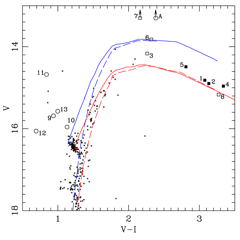
Figure 4: The field-subtracted color-magnitude diagram of stars within 2.5 arcmin of the center of NGC 6496, as described in Sec. 4. Isochrones from (Girardi et al., 2002) having ages of 11.2 Gyr and [Fe/H] = –0.7 (upper) and –0.4 (lower) are shown, with the RGB dashed and the AGB solid. Short-period variables are indicated with circles and LPVs with squares; label numbers give the variable star number, “V#”. The bright variables V7 ($V=12.85$ mag) and ASAS 175901-4411.5 (labeled ”A”, having $V=11.31$ mag) are plotted at fainter magnitudes for convenience in scaling the plot. Solid and open symbols are used for variables located inside and outside a projected radius of 2.5 arcmin from the cluster center, respectively; the former are more likely to be cluster members.

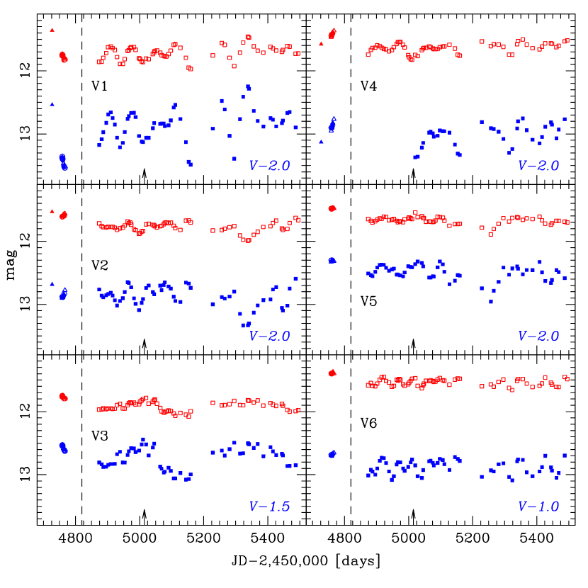
Figure 5: Light curves for the long period variables V1–V6. In each panel, the upper light curve is $I_{L}$ and the lower curve is $V$, shifted upward as indicated for convenience of display. The data to the left of the dashed line were taken at CTIO and are shifted by 4500 days in Julian Date for display. The vertical arrows mark the date at which the P4 image sets were separated due to camera rotation. Photometric errors are smaller than the plot symbols.

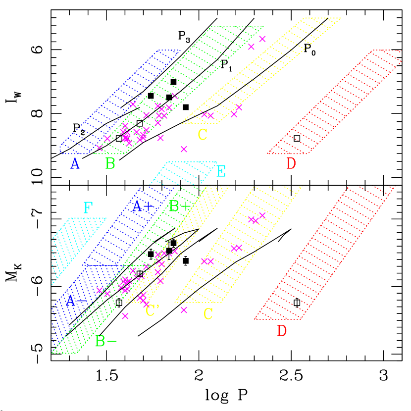
Figure 6: Period-luminosity plots showing (top) $I$-band and (bottom) $K$-band magnitudes, as described in Sec. 5.1. Squares mark LPVs V1-V6 in NGC 6496 inside (filled) and outside (open) a projected radius of 2.5 arcmin, while crosses mark the locations of LPVs in 47 Tuc (Lebzelter & Wood, 2005). The hatched regions mark the sequences of LPVs in the Large Magellanic Cloud shown by Wood et al. (1999) (top) and Ita et al. (2004) (bottom). In both panels, the faintest LPV in NGC 6496, V3, appears in both sequences B and D. The curves in the top panel show pulsation models for LMC stars from Wood et al. (1999) for the fundamental mode ($P_{0}$) and the first through third overtones ($P_{1}-P_{3}$). The curves in the lower panel are $P_{0}-P_{3}$ models (right to left) for pulsating AGB stars undergoing mass loss (Lebzelter & Wood, 2005).

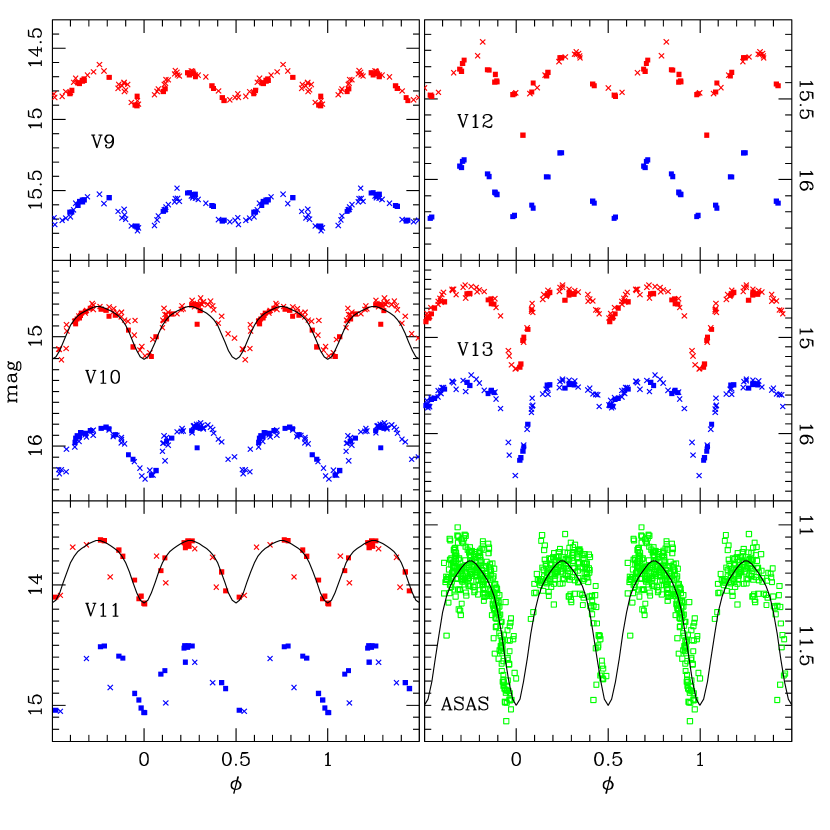
Figure 7: Phased light curves for the short period variables V9–V13 and ASAS 175901-4411.5, with two cycles shown for continuity. In the panels for V9–V13, the upper light curve is $I_{L}$ and the lower curve is $V$, while the solid squares and crosses indicate CTIO and P4 data, respectively. Photometric errors are smaller than the plot symbols. For ASAS 175901-4411.5, the data from the ASAS project are shown. Several panels show the best-fitting template for a W UMa contact binary star.

Table 1: Transformation Coefficients

Set	Filter	$\alpha$	$\epsilon_{\alpha}$	$\beta$	$\epsilon_{\beta}$	RMS
CTIO	$V$	0.273	0.004	0.011	0.010	0.033
CTIO	$I$	0.759	0.007	0.034	0.016	0.052
P4	$V$	-0.612	0.003	0.000	0.000	0.015
P4	$I_{L}$	0.310	0.005	-0.075	0.007	0.020
P4	$I_{S}$	1.910	0.005	-0.095	0.008	0.022

Table 2: Mean Photometry of NGC 6496

ID	$X_{pix}$	$Y_{pix}$	$V$	$\epsilon_{V}$	$I$	$\epsilon_{I}$	Chi	Sharp
1	445.18	21.88	11.306	0.0056	8.904	0.0064	1.031	-0.010
2	714.37	1022.18	10.275	0.0123	10.096	0.0089	1.709	0.035
3	644.07	-67.01	11.215	0.0073	9.812	0.0076	0.994	-0.012
4	491.00	439.53	11.379	0.0054	10.122	0.0055	1.574	-0.049
5	-49.51	406.18	13.098	0.0078	9.619	0.0090	1.516	0.007
6	-34.54	639.31	12.907	0.0069	10.757	0.0076	1.328	-0.006
7	815.93	647.35	12.749	0.0054	11.301	0.0056	1.262	-0.001

Note. — Table 2 is published in its entirety in the electronic edition of the AJ. A portion is shown here for guidance regarding its form and content.

Table 3: Variable Star Coordinates and 2MASS Photometry

V#	IDP4	$X_{P4}$	$Y_{P4}$	$R_{proj}$	RA(J2000)	Dec(J2000)	$J$	$\sigma_{J}$	$K$	$\sigma_{K}$
V1	31	541.4	300.4	2.08	17:58:55.88	–44:14:19.4	9.810	0.024	8.492	0.023
V2	32	240.7	619.3	2.21	17:59:12.94	–44:17:20.5	9.890	0.024	8.543	0.019
V3	29	145.0	527.3	2.64	17:59:17.99	–44:16:24.4	10.458	0.022	9.263	0.019
V4	30	528.0	458.1	1.14	17:58:56.91	–44:15:51.7	9.661	0.024	8.381	0.027
V5	27	419.0	285.8	1.79	17:59:02.55	–44:14:08.3	9.944	0.024	8.642	0.021
V6	18	549.3	839.8	3.85	17:58:56.47	–44:19:36.4	10.035	0.024	8.835	0.021
V7	…	…	…	4.71	17:59:28.01	–44:17:26.7	9.311	0.023	8.195	0.027
V8	…	…	…	5.76	17:59:05.82	–44:21:39.1	10.064	0.022	8.807	0.019
V9	256	930.6	334.7	4.21	17:58:34.68	–44:14:47.1	14.274	0.029	13.893	0.043
V10	244	61.9	841.3	5.89	17:59:23.14	–44:19:27.2	14.028	0.036	13.371	0.035
V11	115	1009.2	543.8	4.95	17:58:30.75	–44:16:51.4	13.265	0.024	12.776	0.023
V12	418	358.1	168.2	2.60	17:59:05.67	–44:12:58.0	14.885	0.040	14.623	0.073
V13	226	841.0	808.8	4.81	17:58:40.44	–44:19:23.9	13.952	0.054	13.419	0.053

Table 4: Time Series Photometry

V#	Time	Phase	$I_{L}$	$\sigma_{L}$	$N_{L}$	$I_{S}$	$\sigma_{S}$	$N_{S}$	$V$	$\sigma_{V}$	$N_{V}$
V1	226.7420	9.999	11.362	0.007	5	99.999	9.999	0	14.537	0.011	5
V1	258.6157	9.999	11.737	0.002	5	99.999	9.999	0	15.376	0.003	5
V1	258.6231	9.999	11.758	0.001	5	99.999	9.999	0	15.381	0.003	5
…	…	…	…	…	…	…	…	…	…	…	…
V1	5487.5210	9.999	11.729	0.006	9	11.748	0.009	9	14.896	0.007	9
V1	5495.5190	9.999	11.725	0.006	9	11.749	0.007	9	99.999	9.999	0
V2	226.7420	9.999	11.534	0.010	5	99.999	9.999	0	14.684	0.009	5
V2	258.6157	9.999	11.606	0.002	5	99.999	9.999	0	14.898	0.003	5
…	…	…	…	…	…	…	…	…	…	…	…
V8	266.8369	9.999	11.882	0.003	5	99.999	9.999	0	15.092	0.003	5
V9	226.7471	0.491	14.777	0.007	5	99.999	9.999	0	15.619	0.005	5
V9	258.6157	0.060	14.899	0.005	5	99.999	9.999	0	15.749	0.004	5
…	…	…	…	…	…	…	…	…	…	…	…
V13	5487.5210	0.192	14.799	0.015	6	14.769	0.029	7	15.703	0.012	6
V13	5495.5190	0.431	14.548	0.005	8	14.554	0.006	8	99.999	9.999	0

Note. — Table 4 is published in its entirety in the electronic edition of the AJ. A portion is shown here for guidance regarding its form and content.

Table 5: Variable Star Properties

V#	$\langle V\rangle$	$\langle I\rangle$	$V_{max}$	$V_{min}$	$I_{max}$	$I_{min}$	$N_{V}$	$P$	$\sigma_{P}$	Type
V1	14.98	11.72	14.25	15.54	11.36	11.97	72	69	2	SR
V2	14.87	11.74	14.60	15.34	11.53	11.99	70	55	3	Lb
V3	14.20	11.89	13.94	14.58	11.74	12.08	71	37	1	Lb
V4	14.98	11.60	14.75	15.37	11.37	11.82	49	73	3	Lb
V5	14.46	11.64	14.30	14.96	11.44	11.89	69	85	15	Lb
V6	13.84	11.51	13.65	14.09	11.36	11.66	69	48	1	Lb
V7	12.85	10.69	12.82	12.88	10.67	10.70	9	…	…	Lb?
V8	15.16	11.90	15.08	15.22	11.88	11.93	16	…	…	Lb?
V9	15.63	14.76	15.51	15.78	14.61	14.90	61	0.76664	0.00005	EW?
V10	15.96	14.83	15.79	16.30	14.65	15.21	78	0.28974	0.00001	EW
V11	14.76	13.85	14.50	15.06	13.63	14.16	27	0.3371	0.0020	EW?
V12	16.04	15.35	15.83	16.25	15.21	15.48	34	0.884	0.001	EW?
V13	15.64	14.68	15.43	16.44	14.46	15.33	78	0.43851	0.0002	EB
ASAS	11.31	8.92	11.15	11.75	…	…	490	740	10	EW?

References

- Alard (2000) Alard, C. 2000, A&AS, 144, 363
- Armandroff (1988) Armandroff, T. E. 1988, AJ, 96, 588
- Baker et al. (2007) Baker, J. M., Layden, A. C., Welch, D. L., & Webb, T. M. A. 2007, AJ, 133, 139
- Clement et al. (2001) Clement, C. M., Muzzin, A., Dufton, Q. et al. 2001, AJ, 122, 2587
- Dotter et al. (2008) Dotter, A., Chaboyer, B., Jevremović, D., Kostov, V., Baron, V., & Ferguson, J.W. 2008, ApJS, 178, 89
- Feast & Whitelock (2000) Feast, M. & Whitelock, P. 2000, in “The Evolution of the Milky Way: stars versus clusters,” eds. Matteucci & Giovannelli, (Kluwer: Dordrecht), 229
- Fourcade & Laborde (1966) Fourcade, C. R. & Laborde, J. R. 1966, “Atlas y Catalogo de Estrellas Variables en Cúmulos Globulares al Sur de -29°,” Córdoba
- Frogel & Whitelock (1998) Frogel, J. A. & Whitelock, P. A. 1998, AJ, 116, 754
- Girardi et al. (2002) Girardi, L., Bertelli, G., Bressan, A., Chiosi, C., Greonewegen, M. A. T., Marigo, P., Salasnich, B., & Weiss, A. 2002, A&A, 391, 195
- Harris (1996) Harris, W. E. 1996, AJ, 112, 1487
- Ita et al. (2004) Ita, Y., Tanabé, T., Matsunaga, N. et al. 2004, MNRAS, 347, 720
- Layden et al. (1999) Layden, A. C., Ritter, L. A., Welch, D. W., & Webb, T. M. A. 1999, AJ, 117, 1313
- Layden et al. (2003) Layden, A. C., Bowes, B. T., & Webb, T. M. A. 2003, AJ, 126, 255
- Lebzelter & Wood (2005) Lebzelter, T. & Wood, P. R. 2005, A&A, 441, 1117
- Nysewander et al. (2009) Nysewander, M., Reichart, D. E., Crain, J. A., Foster, A., Haislip, J., Ivarsen, K., Lacluyze, A., & Trotter, A. 2009, ApJ, 693, 1417
- Olivier & Wood (2005) Olivier, E. A. & Wood, P. R. 2005, MNRAS, 362, 1396
- Percy et al. (2004) Percy, J. R., Bakos, A. G., Besla, G., Hou, D., Velocci, V. & Henry, G. W. 2004, in ASP Conf. Ser. 310, “Variable Stars in the Local Group,” eds. Kurtz & Pollard, (ASP: San Francisco), 348
- Piotto et al. (2007) Piotto, G., Bedin, L. R., Anderson, J., et al. 2007, ApJ, 661, L53
- Pojmanski & Maciejewski (2004) Pojmanski, G. & Maciejewski, G. 2004, Acta Astronomica, 54, 153
- Reichart et al. (2005) Reichart, D., Nysewander, M. Moran, J. et al. 2005, Il Nuovo Cimento C, 28, 767
- Richtler et al. (1994) Richtler, T., Grebel, E. K., & Segewiss, W. 1994, A&A, 290, 412
- Richtler (1995) Richtler, T. 1995, A&AS, 109, 1
- Robin et al. (2003) Robin, A. C., Reylé, C., Derriére, S. & Picaud, S. 2003, A&A, 409, 523
- Sarajedini & Norris (1994) Sarajedini, Ata & Norris, J. E. 1994, ApJS, 93, 161
- Schlafly & Finkbeiner (2011) Schlafly, E. F. & Finkbeiner, D. P. 2011, ApJ, 737, 103
- Smith (1995) Smith, H. A. 1995, “RR Lyrae Stars,” (Cambridge Univ. Press: Cambridge)
- Stellingwerf (1978) Stellingwerf, R. F. 1978, ApJ, 224, 953
- Stetson (1987) Stetson, P. B. 1987, PASP, 99, 191
- Stetson (1994) Stetson, P. B. 1994, PASP, 106, 250
- Stetson (2000) Stetson, P. B. 2000, PASP, 112, 925
- Strutskie et al. (2006) Strutskie, M. F. et al. 2006, AJ, 131, 1163
- Sweigart & Catelan (1998) Sweigart, A. V., & Catelan, M. 1998, ApJ, 501, L63
- Wood et al. (1999) Wood, P. R., Alcock, C. et al. 1999, in IAU Symp. 191, “Asymptotic Giant Branch Stars,” eds. Le Bertre, Lebre, & Waelkens, 151
- Wood, Olivier & Kawaler (2004) Wood, P. R., Olivier, E. A. & Kawaler, S. D. 2004, ApJ, 604, 800
- Zinn & West (1984) Zinn, R. & West, M. J. 1984, ApJS, 55, 45
- Zinn (1985) Zinn, R. 1985, ApJ, 293, 424