Characteristic Length and Clustering
Abstract.
We explore relations between various variational problems for graphs: among the functionals considered are Euler characteristic , characteristic length , mean clustering , inductive dimension , edge density , scale measure , Hilbert action and spectral complexity . A new insight in this note is that the local cluster coefficient in a finite simple graph can be written as a relative characteristic length of the unit sphere within the unit ball of a vertex. This relation will allow to study clustering in more general metric spaces like Riemannian manifolds or fractals. If is the average of scalar curvature , a formula of Newman, Watts and Strogatz [31] relates with the edge density and average scalar curvature telling that large curvature correlates with small characteristic length. Experiments show that the statistical relation holds for random or deterministic constructed networks, indicating that small clustering is often associated to large characteristic lengths and can converge in some graph limits of networks. Mean clustering , edge density and curvature average therefore can relate with characteristic length on a statistical level. We also discovered experimentally that inductive dimension and cluster-length ratio correlate strongly on Erdös-Renyi probability spaces.
Key words and phrases:
Characteristic length, Clustering, Euler characteristic, Variational problems in graph theory1991 Mathematics Subject Classification:
Primary: 05C50,81Q101991 Mathematics Subject Classification:
05C35, 52Cxx1. Introduction
The interplay between global and local properties often appears in geometry. As an example, the Euler characteristic can by Gauss-Bonnet be written as an average of local curvature and by Poincaré-Hopf as an average of local index density for Morse functions . Given a globally defined quantity on a geometric space, one can ask to which extent the functional can be described as an average over local properties. Also of interest is the relation between the various functionals. We will look at some examples on the category of finite simple graphs and comment on both problems. We look then primarily at characteristic length , which is the expectation of local mean distance on a metric space equipped with a probability measure. On finite simple graphs one has a natural geodesic distance and a natural counting measure so that networks allow geometric experimentation on small geometries. Most functionals are interesting also for Riemannian manifolds, where finding explicit formulas for the characteristic length can already lead to challenging integrals. Characteristic length is sometimes also defined as the statistical median of [37]. Since the difference is not essential, we use the averages
where are the number of vertices and edges in the sphere of the vertex .
is the average of the non-local quantity and
is the average of the local quantity giving the fraction of
connections in the unit sphere in comparison to all possible pairs in the unit sphere.
This averaging convention for is common. [10] showed already that
. An other notion is the variance
where for which Ore has shown that on graphs with vertices
has the maximum taken on trees. [11].
The definition of is to average the edge density of the sphere relative to the case
when the sphere is the complete graph with vertices in which case the number
of edges is . Both quantities are natural functionals. The
mean cluster coefficient is by definition an average of local quantities.
While it is impossible to find a local quantity whose average captures
characteristic length exactly, there are notions which come close. We look at three such
relations. The first is a formula of Newman, Watts and Strogatz [31]
which writes as a diffraction coefficient divided by scalar curvature.
This is intuitive already for spheres, where the signal speed and the curvature determines
the characteristic length. Empirically, we find an other quantity which also often allows to estimate
characteristic length well: it is the mean cluster density , the average of a
local cluster density as defined by Watts and Strogatz. Thirdly, we will report on
some experiments which correlate the length-cluster coefficient
with the inductive dimension of the graph.
The starting point of this note is the observation that the local cluster property if a vertex
in a graph can be written in terms of relative characteristic length of the unit sphere within the
unit ball . We are not aware that this has been noted already, but it is remarkable as it allows
to carry over the definition of “local cluster property” to metric spaces equipped with a probability measure
as long as the measure has the property that it induces probability measures on spheres by
conditional probability , where
is an neighborhood of . For such metric spaces, one can also define a
cousin of scalar curvature by comparing the measures
of spheres of radius and . We call it
“scalar curvature” because if is the inductive dimension of space at that point, then
is zero if the volume of the
sphere of radius is equal to times the volume
of a sphere of radius . Comparing with Riemannian manifolds, the comparison of spheres
and allows to measure scalar curvature. The dimension scaling factor does not matter
much because the Hilbert action , the expectation of the scalar
curvature is plus the expectation of . Since the later is a local
function and appears also in a formula of Newman, Watts and Strogatz and because we look at the
dimension anyway, it does not matter if for simplicity is called the
scalar curvature and its average over vertex set is called the Hilbert action
of the graph.
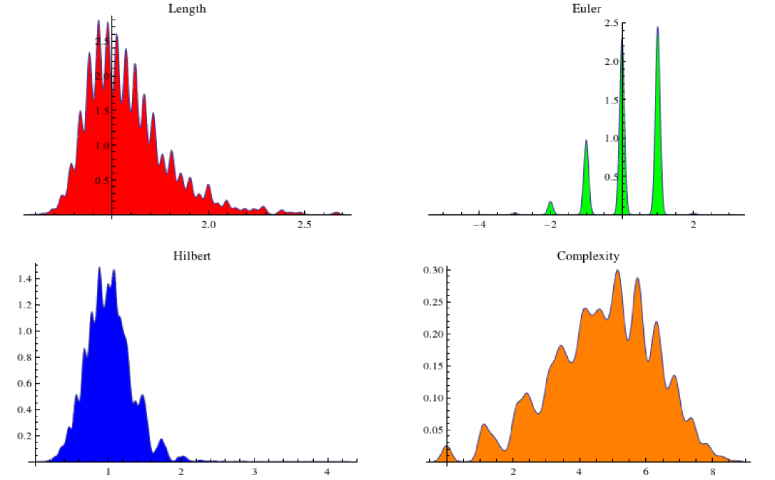
Having these functionals, one can now study the relation between
local cluster property, characteristic length, dimension and curvature on rather general metric spaces
equipped with a natural measure. But first of all these functionals could be used to select “natural
geometries”. Functionals are important in physics because most fundamental laws are of variational nature.
In a geometric setup and especially in graph theory, one can consider the Euler characteristic,
the characteristic length, the Hilbert action given as an average scalar curvature or
the spectral complexity , given as the product of the nonzero eigenvalues of the Laplacian
of . An other related quantity is the number of rooted spanning forests in which is
by the Chebotarev-Shamis theorem
[33, 32, 20, 19].
Many other extremal problems are studied in graph theory [4].
For finite simple graphs, the Euler characteristic
with is the number of dimensional simplices of . In geometric
situations like four dimensional geometric graphs, for which the spheres are discrete three dimensional
spheres, this number can be seen as a quantized Hilbert action [22] because it is an
average of the Euler characteristic over all two-dimensional subgraphs and then via Gauss-Bonnet
an average over a set of sectional curvatures and all points.
The characteristic length is the average length of a path between two points relating
to the other variational problem in general relativity.
The Hilbert action itself is an average of scalar curvature, which can be
defined for a large class of metric spaces. Spectral complexity
is natural because of the matrix tree theorem of Kirkhoff (see i.e. [3] )
relates it with the number of trees in a graph.
While the Euler characteristic is an average of curvature by Gauss-Bonnet both in the Riemannian
and graph case [16] and Hilbert action is an average of scalar curvature,
both the characteristic length as well as the complexity can not be written
as an average of local properties: look at two disjoint graphs connected along a
one-dimensional line graph. Cutting that line in the middle can change both quantities in a very different way
depending on the two components which are obtained. If
or were local, the functional would change by a definite value, independent of the length of the “rope”.
The characteristic length has been noted to be relevant for molecules: the chemist Harry Wiener found
correlations between the Wiener index , the sum over all distances which is
and the melting point of a hydrocarbon . As reported in
[13], the characteristic length has first been considered in
[10] in graph theory. For spectral properties, see [29].
The observation that the Wiener index satisfies
for any spanning tree of was made in [34].
The characteristic length has been studied quite a bit. There are few classes of
graphs, where one can compute the number explicitly: for complete graphs, we have
for complete bipartite graphs
for line graphs , for cyclic graphs .
for odd and if is even [11].
No general relation between length and diameter exists besides the trivial .
We have [10],
On the class of graphs with vertices and edges
one has [11].
Among all graphs with vertices the maximum is obtained for line graphs, the minimum
for complete graphs [10]. The problem to find the maximum among all graphs of given
order and diameter is unknown. There are relations with the spectrum: on
where is the number of distinct Laplacian eigenvalues. There are also upper bounds in terms of the second
eigenvalue.
For a connected graph where is the independence number [8],
the maximal number of pairwise nonadjacent vertices in .
On all graphs of order and minimal degree , then [28].
The conjecture generating computer program Graffiti [12]
suggested for constant degree graphs to have .
There is a spectral relation, where
is the Moore pseudo inverse of the Laplacian and the number of vertices( [35]
which is the McKay equality for trees and otherwise always a strict inequality.
The Euler characteristic is definitely one of most important functionals in geometry if not the
most important one. It is a homotopy invariant and can by Poincaré-Hopf be expressed cohomologically
as using the dimensions of cohomology groups .
A general theme in topology is to extend the notion of Euler characteristic to larger classes of
topological spaces. This essentially boils down to the construction of cohomology.
The limitations are clear already in simple cases like the Cantor set which have
infinite Euler characteristic as half of the space is homeomorphic to itself. Euler characteristic
can be defined for a metric space if there exists a subbasis of contractible graphs. The
Euler characteristic can then be defined as the Euler characteristic of the nerve graph. This
illustrates already how important homotopy is in general when studying Euler characteristic.
It is also historically remarkable that the first works done by Euler on Euler characteristic
were of homotopy nature by deforming the graph.
Various other functionals have been considered on graphs. The average centrality is the mean of the local closeness centrality
of a vertex . An other number is the geodetic number which is the minimum
cardinality of a geodetic set in , where a set is called geodetic if its geodesic closure
is [1]. The scale measure of a graph is defined as , where
and and .
An other important notion is the chromatic number which can be seen as the smallest
for which a scalar function with values in exists for which the gradient
field nowhere vanishes. Related to graph coloring, we have in [25] defined
chromatic richness measuring the size of the set of coloring functions modulo permutations.
The arboricity of is the minimal number of spanning forests
which are needed to cover all edges of . One knows that by
Chebotarev-Shamis [33, 32, 20, 19].
While the number of spanning forests is a measure of complexity, the arboricity is a measure of
“denseness” of the graph. The Nash-Williams formula [30, 7]
tells that the arboricity is the maximum of , where
is the number of vertices and the number of edges of a subgraph of and where is
the ceiling function giving the minimum of all integers larger or equal than . For example,
for where the arboricity must be at least and so at least
and one can give examples of three forests covering all edges.
For a complete graph, the arboricity is . The arboricity gives a bound on
the chromatic number (a fact noted in [6] and follows
from the fact that each forest can be colored by 2 colors).
The Laplacian ratio ,
where is the
permanent of the Laplacian and are the vertex degrees has been introduced in [5].
The symmetry grade of a graph is the order of the automorphism group of . For the complete graph
for example, it is while for a cyclic graph it is , the size of the dihedral group.
The domatic number of a graph finally is the maximal size of a dominating partition of
the vertex set.
| Functional | Based on | Local | Spectral | |
|---|---|---|---|---|
| Euler characteristic | Curvature | yes | somehow [18] | |
| Inductive dimension | Point dimension | yes | not known | |
| Characteristic length | Distance | no | on trees [13] | |
| Complexity | Eigenvalues | no | yes | |
| Forest complexity | Eigenvalues | no | yes | |
| Hilbert action | Scalar curvature | yes | not known | |
| Mean cluster | Local cluster | yes | yes | |
| Average degree | Vertex degree | yes | yes | |
| Graph density | Edge number | yes | yes | |
| Scale measure | Vertex degree | yes | not known | |
| Cluster-length-ratio | Distances | no | not known | |
| Independence number | Adjacency | no | not known | |
| Variance | Distance | no | not known | |
| Centrality | Local centrality | yes | not known | |
| Chromatic number | Gradient fields | no | no [9] | |
| Arboricity | Forests | no | not known | |
| Geodetic number | Geodesics | no | not known | |
| Domatic number | Partitions | no | not known | |
| Symmetry grade | Symmetry group | no | not known | |
| Laplacian ratio | Permanent | no | not known |
Besides the question whether a functional is local, it would also be interesting to know more about which properties are spectral properties. Euler characteristic can be seen as a spectral property in the wider sense: it is the super trace of for the Dirac operator for every by McKean-Singer [18]. The average degree can be written in terms of the adjacency matrix as and with the Laplacian as . The graph density is also spectral, because both and are spectral.
2. Characteristic length
A finite simple graph defines a finite metric space, where is the geodesic distance between two vertices , the length of the shortest path connecting the two points. The characteristic length is the expectation of the distances between different vertices , where is the number of vertices. We have the understanding that the graph with only one vertex has zero length and that the number is averaged over every connected component of a graph independently. Unlike the Euler characteristic which is a homotopy invariant, the global characteristic length is a metric property as it depends on the concrete metric and is only invariant under graph isomorphisms and not under topological homeomorphisms [27] nor homotopies. Since determining requires to map out all the distances between any two points, it is natural to ask whether one can estimate the global length by averaging local properties. Such a relation has appeared in “formula 54” of [31],
where it was derived from generating functions. ‘Formula 54” uses the average degree (the average of the degrees ) and the average -nearest neighbors (the average of the size of the spheres of radius ). Because by Euler’s handshaking lemma, we know that agrees with the edge density . Since measures a relation between volumes of spheres of distance and , it can intuitively be thought of a scalar curvature, the flat case meaning the volume of the sphere of radius being larger than times the volume of the sphere of radius which has dimension , where denotes the dimension of the vertex . The global characteristic length is according to ”formula 54” an ”edge density/curvature” relation which is intuitive because distances are small in spaces of positive curvature and the fact that if a material has large edge density, it allows fast travel. To summarize, ”formula 54” relates the edge density , the Hilbert action and the characteristic length as
where
is the average of shifted scalar curvature .
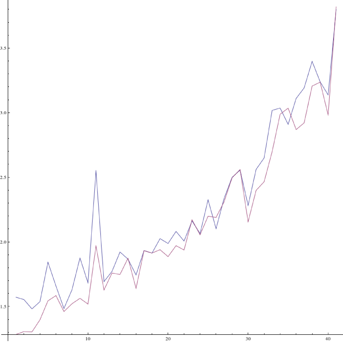
Empirically, we also see a close relation between and , where is the mean
cluster coefficient as defined by [38]. We have mentioned this in
[14] (see also [26, 24]). Clustering is a notion
which is related to transitivity in sociology [36]. We see in many natural networks
that these two quantities and grow linearly with with a similar
order of magnitude. Since can be expressed integral geometrically
using lengths, it can be pushed to natural metric spaces like compact Riemannian
manifolds or metric spaces with fractal dimension.
Why is the characteristic length interesting? In physics, is minimized by geodesics connecting with so that averages over all possible Lagrangian actions of paths between any two points. General relativity builds on two variational pillars: one is the Hilbert action , the average scalar curvature, the other is the geodesic variational problem to minimize geodesic length between two points. The first tells how matter determines geometry, the second describes how geometry influences matter. “Formula 54” indicates a statistical correlation between Hilbert action, edge density and characteristic length. Since scalar curvature appears in the expansion , we can express this without referring to Euclidean space as
so that
Since and are averages, the mean field approximations are
only expected to be good in some mean field sense.
We would like to know more about the relation between Euler characteristic ,
graph density , dimension , complexity , clustering
and characteristic length . Also interesting are relations with corresponding notions
of Riemannian manifolds.
Besides average length and dimension, complexity makes sense for Riemannian manifolds too, even so it
needs zeta regularized determinants for its definition.
The mean clustering is proportional to the volume with a proportionality factor which depends
on the dimension. For a Riemannian manifold, scaling the space by a factor scales the
characteristic length in the same way and the volume by a factor . For random networks,
the global characteristic length
typically grows like in dependence of volume - one aspect of the “small world” phenomenon.
This does not violate geometric intuition at all because dimension grows too with more nodes.
We have explicit formulas [15] for the average dimension of a random
Erdös-Renyi graph of size , where edges are turned on with probability .
For other random graphs like Watts-Strogatz networks or networks generated by random permutations,
we see similar growth rates. Other type of networks can show slightly different growth rates.
Barabasi-Albert networks are examples, where the growth rate is slower.
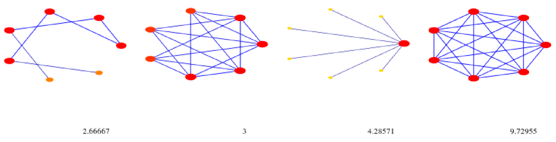
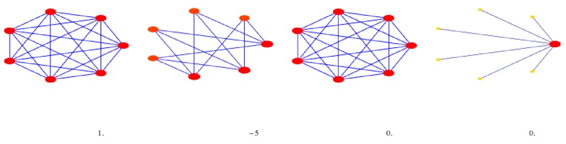
Related to characteristic length is the magnitude , where defined by Solow and Polasky. We numerically see that at least for small vertex cardinality and connected graphs, the complete graph has minimal magnitude and the star graph maximal magnitude, a feature which is shared for many functionals (see Figure 2). Also the magnitude can be defined for more general metric spaces so that one can look for a general metric space at the supremum of all where is a finite subset with induced metric. The convex magnitude conjecture of Leinster-Willington claims that for convex subsets of the plane, , where is the perimeter and is the area.
3. Local cluster coefficient
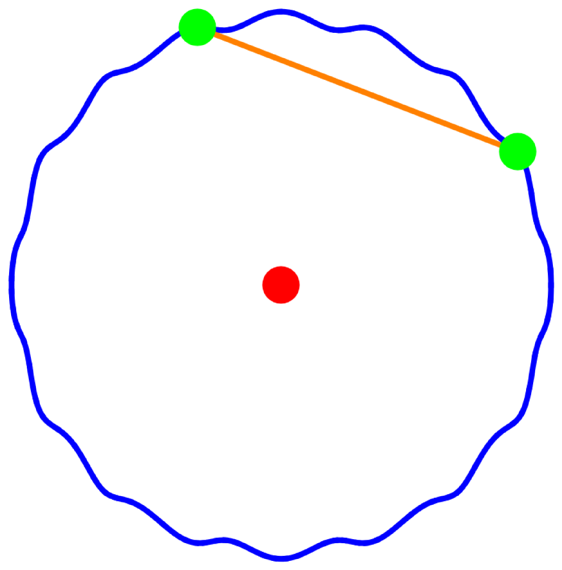
Given a subgraph of a graph , define the relative characteristic length as
The difference is nonnegative. It is zero if all geodesics
connecting two points in remain in . The notion makes sense in any metric
space equipped with a probability measure. The number is a measure for how
far is away from being convex within the metric space . The notion depends on a choice
of a probability measure on . On graphs, many fractal sets, spaces on which a Lie group
acts transitively or Riemannian manifolds, there is a natural measure.
Examples:
1) For a compact surface in three dimensional space for example,
is zero if and only if is a plane. We understand that the average has been
formed with respect to some absolutely continuous probability measure on the surface
which gives positive measure to every open set.
2) For a curve in a compact Riemannian
manifold , the relative characteristic length is if the curve is a short
enough geodesic. But the relation will decrease eventually to zero for
aperiodic geodesic paths as the geodesic will accumulate.
3) For a region in Euclidean space, we have if and
only if is convex in in the sense that for any two points
there is a geodesic in which is also in .
Define the local characteristic length as
where is the unit sphere and is the unit ball of the vertex . We always
assume that the space is large enough so that the unit ball at every point is convex within
in the above sense.
The quantity is defined therefore for large enough
metric spaces equipped with a probability measure which is nice enough that
it induces measures on spheres by limiting conditional expectation. Examples
are Riemannian manifolds or graphs.
For a finite simple graph , the local cluster coefficient is defined as
where is the set of edges in the unit sphere of and
is the set of vertices in . The mean cluster coefficient was defined
by Watts-Strogatz is the average of over all . The local cluster
coefficient gives the edge occupation rate in the sphere of a vertex .
Other related quantities are the global cluster coefficient
defined as the frequency of oriented triangles within
all oriented connected vertex triples. The transitivity ratio is the ratio
of non-oriented triangles within the class of non-oriented connected vertex triples in .
We do not look at the later two notions because they are close to the mean cluster
density and because intuition about them is more difficult.
We can define higher global cluster coefficients of a graph as the fraction , where is the number of -dimensional simplices in and the number of connected -tuples of vertices. Of course, is the global clustering coefficient and is the local clustering coefficient at a point . One could define higher local clustering coefficient as the global clustering coefficient . There are also higher dimensional characteristic lengths: define as the distance between two -dimensional simplices , where the distance is the smallest such that we can connect with a sequence of overlapping simplices . Of course is the usual geodesic distance and for geometric graphs of dimension all distances are essentially the same. For a triangularization of a Riemannian manifold, where every sphere is one-dimensional cyclic graph, the distance between two triangles which overlap is . We mentioned these higher clustering coefficients and higher characteristic lengths because we believe they could be used to get a closer relation with inductive dimension which also uses the entire spectrum of higher dimensional simplices and not only zero dimensional vertices and one dimensional edges.
4. Cluster coefficient and local length
While the following observation is almost obvious, we are not aware that it has been noticed anywhere already. The result allows to write the local cluster coefficient in terms of the relative characteristic length of the unit sphere within the unit ball . This will allow us to push the notion of local clustering coefficient to other metric spaces equipped with natural measures. Just define then there.
Lemma 1 (Cluster-Length-Lemma).
.
Proof.
By definition, the distance function takes only two different positive values in the ball . The first possibility is which is the case if one of the vertices is the center. The second possibility is if both are on the sphere. If is the degree of the vertex then has vertices and has vertices. The distance appears times on the sphere . The distance appears times in the sphere . The average is
∎
An extremal case is a star graph which has cluster coefficient and dimension
and where the distance between any two points of the unit sphere is .
An other extreme case is the complete graph which has the cluster coefficient
and dimension , where the distance between any two points of the unit sphere is .
The wheel graph is an example in which each point has a -dimensional sphere, the local cluster coefficient of the center is and of the other points . The mean cluster coefficient for is . The cluster-length-ratio is close to .
5. Dimension
An other important local quantity is the dimension of a vertex and the inductive dimension of a graph, the average dimension of its vertices. It was defined in [17] as
where
denotes the unit sphere of a vertex .
Already on a local level, there can be relations. If the dimension of a point is zero,
then clearly the local length is and the cluster coefficient is zero. And
also is zero.
We have shown in [15]
that the expectation on satisfies the recursion
where . Each is a polynomial in of degree .
6. Metric spaces
The characteristic length of a metric space with measure
is the expectation of length on , where is the
diagonal in . The local length
is the characteristic length of the unit sphere within the unit
ball . Motivated by the above, we call the local cluster coefficient
of the pint in and its expectation , the mean cluster coefficient.
Lets look at the quantity , where is the radius of the small ball and
where the volume of the manifold is . These are integral geometric questions. We
in general assume that is scaled in such a way that the radius of injectivity is
larger than and the unit ball is contractible and convex. For a Riemannian manifold, the
number is a dimension-dependent constant, the average distance between two points in the
unit sphere. For manifolds, studying is therefore equivalent than to study the
characteristic length. The question is however interesting for fractals. One can ask for
example, what the cluster-length ration is for the Sirpinsky carpet.
Example 1. For a flat torus with flat Riemannian geodesic distance and area measure, we have
and . Therefore,
Example 2. Also for a three-dimensional flat torus, the clustering
coefficient is constant and given as the average distance of two points
on a sphere, which is . The characteristic length on the other hand is ,
a numerical integral which we were not able to evaluate analytically. The
quotient is .
Example 3. For a two-dimensional sphere of surface area , the characteristic length is times the characteristic length of the unit sphere which is intrinsic and uses the geodesic length within the surface and not from an embedding. We measure it in to be so that can be computed by using that that the geodesic distance between two points given in spherical coordinates as is given by the Haverside formula where is the Haverside function. Random points on the sphere can be computed with the uniform distribution in and the distribution in . Assuming the same value as in the plane (which uses that near a specific point we can replace the sphere with its tangent space) and get .
7. Cluster-length ratio
Dimension plays a role for characteristic length. We measure experimentally that the global length-cluster ratio quantity
is correlated to dimension for Erdös-Renyi graphs:
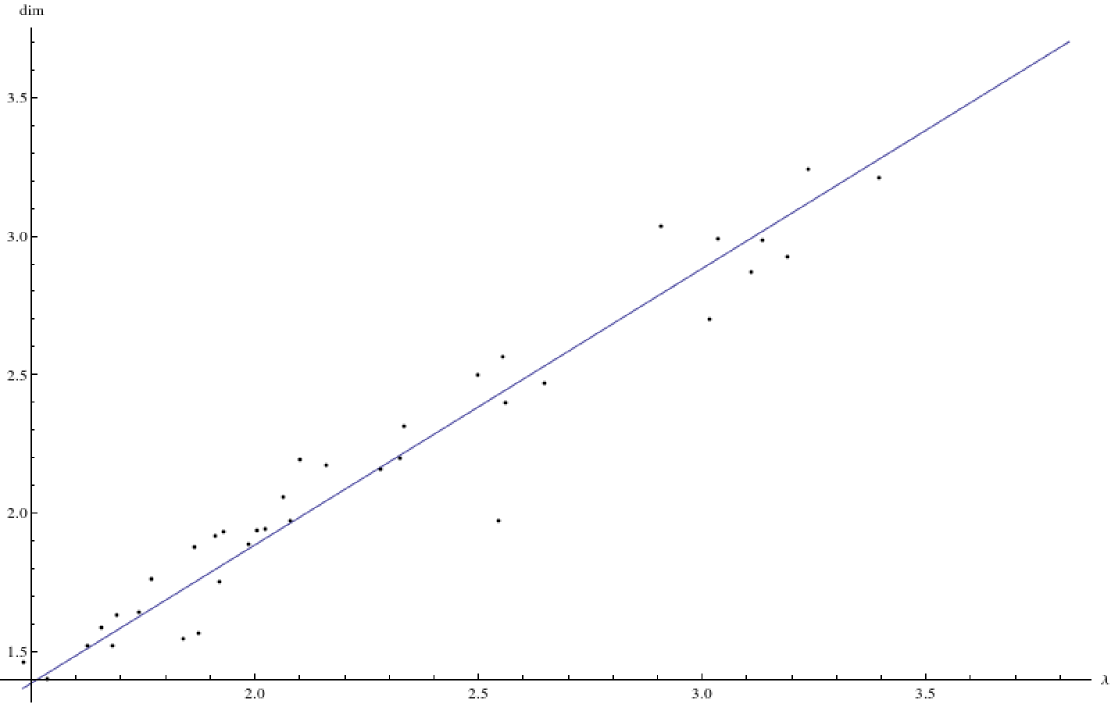
Here is some intuition, why the limit should exist: the cluster coefficient is related to the existence of triangles in the graph. For orbital networks [21, 23, 24] defined by polynomial maps the number of triangles is bounded by a constant . This implies that and for orbital networks, we should get that has a finite interval as accumulation points. To show that grows like , we don’t want too many relations with different words . We call this a collision. If is the number of generators, then, if there were no collisions, the relation holds. With double collisions, assuming no triple collisions, we have the relation and so . Together with we have . So, if we can show to be of the order and the number of triangles to be of the order , and triple collisions are rare, then we should be able to prove that the limit exists.
8. Classes of networks
The space of all graphs on a vertex set with nodes, where every node is turned on with probability is a probability space. The limit
for exists almost surely. We see that the value is
close to , where is the radius of the graph and is
the dimension of the network.
The quotient (8) is interesting because
is a global property and is the average of a local property.
Intuitively, such a relation is to be expected because a larger allows to tunnel
faster through a ball and allows for shorter paths. If the limit exists,
then .
Knowing is important because the characteristic length is more costly to compute
while the clustering coefficient is easier to determine as a simple average
of local quantities.
To allow an analogy from differential geometry, we could compare with curvature, because a
metric space with larger curvature has a smaller
average distance between two points on the unit sphere.
We could look at graphs with a given dimension and volume and minimize the average path length between two points among all graphs. It is a long shot but one can ask whether there is the relation between graphs minimizing and graphs minimizing Euler characteristic . We can only explore this so far for very small graphs. The reason for asking this is that Euler characteristic can also been seen as an average of scalar curvature and therefore a quantized Hilbert action [22].
9. Related questions
Variational problems on graphs usually need some constraints because the functionals are often
trivial without restrictions. We can restrict the
number of vertices or edges and look at the maximum or minimum on that space.
More generally, we can use a Lagrange type problem and look at all the graphs for which one
functional is constant and extremize the other on that class. This leads to more
questions and most of them seem not have been studied. Instead of restricting to a “level surface”
we can also look at the functionals on an equivalence class of graphs. One interesting
example is to look at homotopy as an equivalence relation. A homotopy step is given by
choosing a contractible subgraph of and connect each vertex of with a new vertex .
An other homotopy step is the reverse operation: remove a vertex for which the unit sphere is
contractible. The notion of contractible if a sequence of homotopy steps transforms it to a one
point graph.
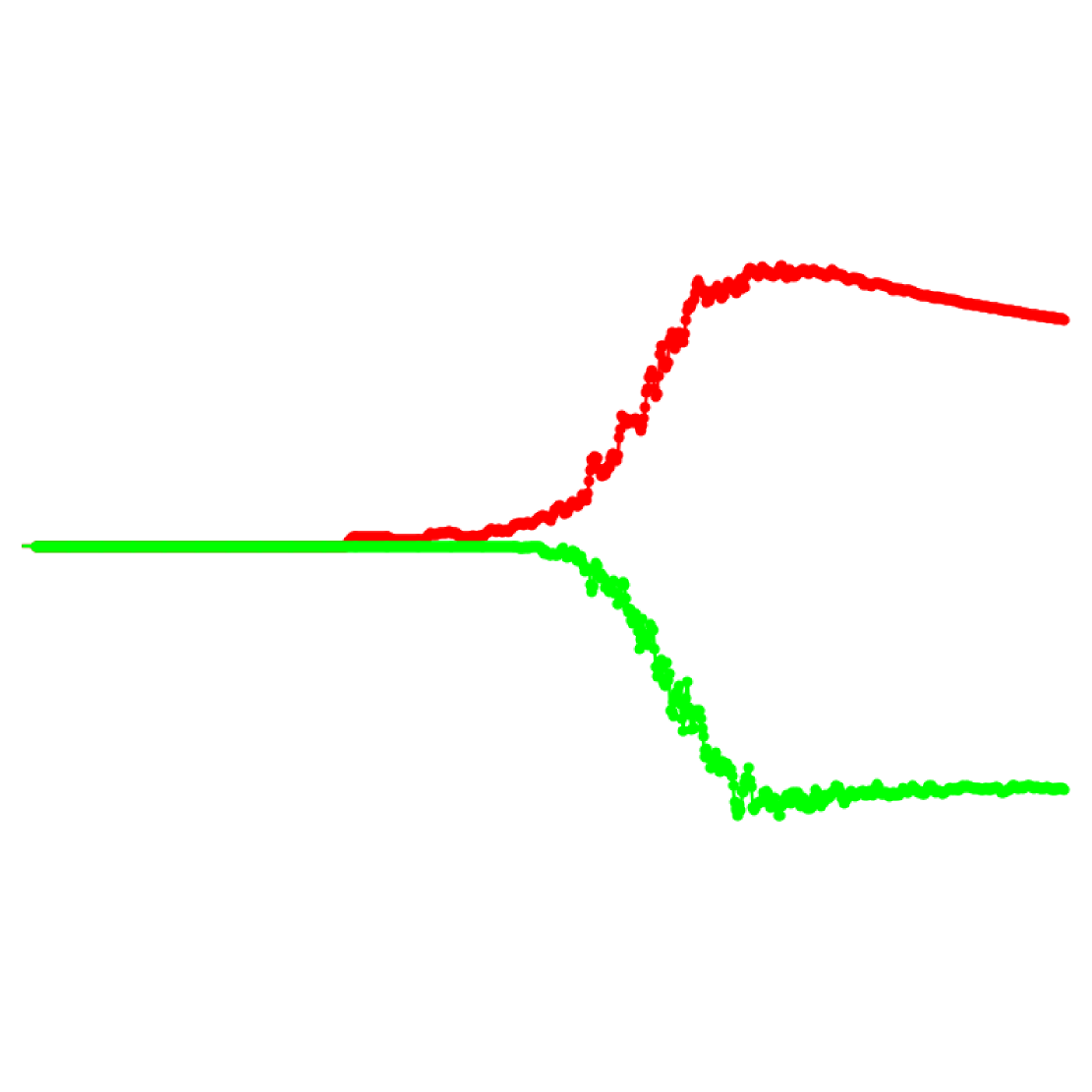
Lets look at the example of minimizing the dimension in a homotopy class. The
homotopy class of a circle contains graphs of arbitrary
large dimension; it contains for example
discretization of a solid torus (dimension 3) or an annulus (dimension 2).
We can also find one-dimensional graphs homotopic to the circle which are not .
We can for example attach one dimensional hairs to the circle without changing dimension,
nor homotopy. We have now a new functional which is the minimal dimension
among all graphs homotopic to . For a contractible graph, the minimal dimension
is . On the class of graphs homotopic to the circle the minimal dimension
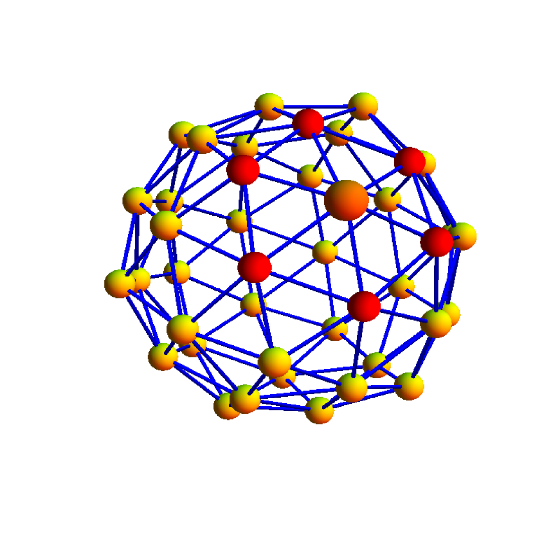
is and for all graphs homotopic to an icosahedron it is .
A similar modified dimension can be defined
in the continuum: define the homotopy dimension of a space as the minimum of
the Hausdorff dimensions of all compact metric spaces homotopic to .
The question is whether the minimum is always attained by a geometric graph or smooth manifolds.
References
- [1] M. Kovse B. Bresar and A. Tepeh. Geodetic sets in graphs. In M. Dehmer, editor, Structural Analysis of Networks. Birkhäuser, 2011.
- [2] A-L. Barabási and R. Albert. Emergence of scaling in random networks. Science, 286(5439):509–512, 1999.
- [3] N. Biggs. Algebraic Graph Theory. Cambridge University Press, 1974.
- [4] B. Bollobas. Extremal Graph Theory. Dover Courier Publications, 1978.
- [5] R.A. Brualdi and J.L. Goldwasser. Permanent of the laplacian matrix of trees and bipartite graphs. Discrete Mathematics, 48:1–2, 1984.
- [6] S. Butler. Relating the arboricity with the chromatic number of a graph. http://www.math.iastate.edu/butler/PDF/arboricity.pdf, accessed, July 20, 2014.
- [7] B. Chen, M. Matsumoto, J. Wang, Z. Zhang, and J. Zhang. A short proof of nash-williams’ theorem for the arboricity of a graph. Graphs and Combinatorics, 10:27–28, 1994.
- [8] F.R.G. Chung. The average distance and independence number. J. Graph Theory, 12:229–235, 1988.
- [9] D.M. Cvetkovic. Chromatic number and the spectrum of a graph. Publications de l’insitute Mathematique, 14(28):25–38, 1972.
- [10] J. Doyle and J. Graver. Mean distance in a graph. Discrete Math, 17:147–154, 1977.
- [11] R.C. Entringer, E.E. Jackson, and D.A. Snyder. Distance in graphs. Czechoslovak Mathematical Journal, 26:283–296, 1976.
- [12] S. Fajtlowicz. Toward fully automated fragments of graph theory. Graph Theory Notes N. Y., 42:18–25, 2002.
- [13] W. Goddard and O.R. Oellermann. Distance in graphs. In M. Dehmer, editor, Structural Analysis of Networks. Birkhäuser, 2011.
- [14] O. Knill. Natural orbital networks. http://arxiv.org/abs/1311.6554.
-
[15]
O. Knill.
The dimension and Euler characteristic of random graphs.
http://arxiv.org/abs/1112.5749, 2011. -
[16]
O. Knill.
A graph theoretical Gauss-Bonnet-Chern theorem.
http://arxiv.org/abs/1111.5395, 2011. - [17] O. Knill. A discrete Gauss-Bonnet type theorem. Elemente der Mathematik, 67:1–17, 2012.
-
[18]
O. Knill.
The McKean-Singer Formula in Graph Theory.
http://arxiv.org/abs/1301.1408, 2012. -
[19]
O. Knill.
A cauchy-binet theorem for Pseudo determinants.
http://arxiv.org/abs/1306.0062, 2013. - [20] O. Knill. Counting rooted forests in a network. http://arxiv.org/abs/1307.3810, 2013.
- [21] O. Knill. Dynamically generated networks. http://arxiv.org/abs/1311.4261, 2013.
- [22] O. Knill. The Euler characteristic of an even-dimensional graph. http://arxiv.org/abs/1307.3809, 2013.
- [23] O. Knill. Natural orbital networks. http://arxiv.org/abs/1311.6554, 2013.
- [24] O. Knill. On quadratic orbital networks. http://arxiv.org/abs/1312.0298, 2013.
- [25] O. Knill. Curvature from graph colorings. http://arxiv.org/abs/1410.1217, 2014.
- [26] O. Knill. Dynamically generated networks. 2014. http://arxiv.org/abs/1311.4261.
- [27] O. Knill. A notion of graph homeomorphism. http://arxiv.org/abs/1401.2819, 2014.
- [28] M. Kouider and P.Winkler. Mean distance and minimum degree. J. Graph Theory, 25(1):95–99, 1997.
- [29] P. Van Miegham. Graph spectra for complex networks. 2011.
- [30] C. Nash-Williams. Edge-disjoint spanning trees of finite graphs. J. London Math. Soc., 36:455–450, 1961.
- [31] M.E.J. Newman, S.H. Strogatz, and D.J. Watts. Random graphs with arbitrary degree distributions and their applications. Physical Review E, 64, 2001.
- [32] P.Chebotarev and E. Shamis. Matrix forest theorems. arXiv:0602575, 2006.
- [33] E.V. Shamis P.Yu, Chebotarev. A matrix forest theorem and the measurement of relations in small social groups. Avtomat. i Telemekh., 9:125–137, 1997.
- [34] N.S. Schmuck. The wiener index of a graph. Diploma thesis, TU Graz, 2010.
- [35] S. Sivasubramanian. Average distance in graphs and eigenvalues. Discrete Mathematics, 309:3458–3462, 2009.
- [36] S. Wasserman and K. Faust. Social Network analysis: Methods and applications. Cambridge University Press, 1994.
- [37] D. J. Watts. Small Worlds. Princeton University Press, 1999.
- [38] D. J. Watts and S. H. Strogatz. Collective dynamics of ’small-world’ networks. Nature, 393:440–442, 1998.